Delay-Throughput Tradeoff for Supportive Two-Tier Networks

Abstract

Consider a static wireless network that has two tiers with different priorities: a primary tier vs. a secondary tier. The primary tier consists of randomly distributed legacy nodes of density $n$, which have an absolute priority to access the spectrum. The secondary tier consists of randomly distributed cognitive nodes of density $m=n^{\beta}$ with $\beta\geq 2$, which can only access the spectrum opportunistically to limit the interference to the primary tier. By allowing the secondary tier to route the packets for the primary tier, we show that the primary tier can achieve a throughput scaling of $\lambda_{p}(n)=\Theta\left(1/\log n\right)$ per node and a delay-throughput tradeoff of $D_{p}(n)=\Theta\left(\sqrt{n^{\beta}\log n}\lambda_{p}(n)\right)$ for $\lambda_{p}(n)=O\left(1/\log n\right)$, while the secondary tier still achieves the same optimal delay-throughput tradeoff as a stand-alone network.

I Introduction

The explosive growth of large-scale wireless applications motivates people to study the fundamental limits over wireless networks. Consider a randomly distributed wireless system with density $n$ over a unit area, where the nodes are randomly grouped into one-to-one source-destination (S-D) pairs. Initiated by the seminal work in [1], the throughput scaling laws for such a network have been studied extensively in the literature [2]-[4]. For static networks, it is shown [1] that the traditional multi-hop transmission strategy can achieve a throughput scaling of $\Theta\left(1/\sqrt{n\log n}\right)$ per S-D pair. Besides the throughput, the packet delay is another key performance metric in wireless networks. The delay-throughput tradeoffs for static and mobile networks have been investigated in [5]-[7]. Specifically, for static networks, it is shown in [7] that the optimal delay-throughput tradeoff is given by $D(n)=\Theta(n\lambda(n))$ for $\lambda(n)=O\left(1/\sqrt{n\log n}\right)$, where $D(n)$ and $\lambda(n)$ are the delay and throughput per S-D pair, respectively.

The aforementioned literature focuses on the delay and throughput scaling laws for a single network. Recently, the emergence of cognitive radio networks leads to the necessity of extending the result from a single network to multiple overlaid networks. Consider a licensed primary network and a cognitive secondary network coexisting in a unit area. The primary network has the absolute priority to use the spectrum, while the secondary network can only access the spectrum opportunistically such that the resulted interference to the primary network is tolerable. Based on such assumptions, the delay and throughput performance for the two overlaid networks have been studied in [8] [9]. In [8], it has been shown that by defining a preservation region around each primary node, both networks can achieve the same throughput scaling law given in [1] as a stand-alone wireless network. In [9], it has been further shown that both networks achieve the same delay-throughput tradeoff as the optimal one established in [7]. However, these existing results are obtained without considering possible positive interactions between the primary network and the secondary network. In practice, the secondary network, which is usually deployed after the existence of the primary network for opportunistic spectrum access, can transport not only its own data packets but also the packets for the primary network. As such, a natural question arises whether the throughput and/or delay performance of the primary network can be improved via the aid of the newly-added secondary network, without the need of modifications over the existing primary protocol. Meanwhile, we study whether the the secondary network is still capable of keeping the same throughput and delay scaling laws as in a stand-alone network.

In particular, we consider the primary network and the secondary network as two coexisting tiers with different priorities (a legacy tier vs. a cognitive tier) in a wireless system, where each of them has its own data packets to transmit such that we need to evaluate the performance of the two tiers respectively. In such a system, we allow the secondary tier to supportively relay the data packets for the primary tier in an opportunistic way, while the primary tier is only required to transmit its own data. Furthermore, we require the primary protocol to keep the same as in a legacy single-tier network given the fact that the primary tier may already exist before the secondary tier is added in. Based on these assumptions, we deploy a similar primary protocol to those in [1] [8] [9] and propose a new multi-hop transmission protocol for the secondary tier. We show that when the secondary tier has a higher density than the primary tier, i.e., $m=n^{\beta}$ with $\beta\geq 2$, the throughput scaling law of the primary tier can be significantly improved from $\Theta\left(1/\sqrt{n\log n}\right)$ to $\Theta\left(1/\log n\right)$ per S-D pair with the aid of the secondary tier, while the secondary tier can still achieve the throughput scaling law of $\Theta\left(1/\sqrt{m\log m}\right)$ per S-D pair as a stand-alone network. Furthermore, we investigate the delay performance and the delay-throughput tradeoff within each tier.

The rest of the paper is organized as follows. The system model is described in Section II. The proposed protocols for the primary and secondary tiers are described in Section III. The delay and throughput scaling laws for the secondary tier are shown in Section IV. The delay and throughput scaling laws for the primary tier are shown in Section V. Finally, Section VI summarizes our conclusions.

II System Model

In this section, we first describe the network model and the system assumptions, and then define the transmission rate and throughput. In the following, we use $p(E)$ to represent the probability of event $E$, and claim that an event $E_{n}$ occurs with high probability (w.h.p.) if $p(E_{n})\to 1$ as $n\to\infty$.

II-A Network Model

Consider two network tiers over a unit square. The nodes of the primary tier, so-called primary nodes, are distributed according to a Poisson point process (PPP) of density $n$ and randomly grouped into one-to-one source-destination (S-D) pairs. Likewise, the nodes of the secondary tier, so-called secondary nodes, are distributed according to a PPP of density $m$ and randomly grouped into S-D pairs. We assume that the density of the secondary tier is higher than that of the primary tier, i.e.,

$$m=n^{\beta}$$ (1)

where we consider the case $\beta\geq 2$. The primary tier and the secondary tier share the same time, frequency, and space, but have different priorities to access the spectrum: The former one is the licensed user of the spectrum and thus has a higher priority; and the latter one can only opportunistically access the spectrum to limit the resulting interference to the primary tier.

For the wireless channel, we only consider the large-scale pathloss and ignore the effects of shadowing and small-scale multipath fading. As such, the channel power gain $g(r)$ is given as

$$g(r)=r^{-\alpha}$$ (2)

where $r$ is the distance between the transmitter (TX) and the corresponding receiver (RX), and $\alpha>2$ denotes the pathloss exponent.

II-B Interaction Model

As shown in the previous work [8] [9], although the opportunistic data transmission in the secondary network does not degrade the scaling law of the primary network, it may reduce the throughput in the primary tier by a constant factor due to the fact that the interference from the secondary network to the primary network cannot be reduced to zero. To completely compensate the throughput degradation or even improve the throughput scaling law of the primary tier in a two-tier setup, we could allow certain positive interactions between the two tiers. Specifically, we assume that the secondary tier is willing to route packets for the primary tier, while the primary tier is not assumed to do so. In particular, when a primary node sends packets, the surrounding secondary nodes could pretend to be primary nodes to relay the packets. After a secondary node receives the packets from a primary node, it may chop the packets into smaller pieces suitable for secondary-tier transmissions. The small data pieces will be assembled before they are delivered to the primary destination nodes. Note that, these “fake” primary nodes do not have the same priority as the real primary nodes in terms of spectrum access, i.e., they can only use the spectrum opportunistically in the same way as a regular secondary node. As such, the primary tier is expected to achieve a more efficient throughput scaling law. The assumption of allowing packet exchanges between the two tiers is the essential difference from the models in [8] [9].

II-C Throughput and Delay

The throughput per S-D pair is defined as the average data rate that each source node can transmit to its chosen destination as in [8] [9], which is a function of the network density. Besides, the sum throughput is defined as the product between the throughput per S-D pair and the number of S-D pairs in the network. In the following, we use $\lambda_{p}(n)$ and $\lambda_{s}(m)$ to denote the throughput per S-D pair for the primary tier and the secondary tier, respectively; we use $T_{p}(n)$ and $T_{s}(m)$ to denote the sum throughputs for the primary tier and the secondary tier, respectively.

The delay of a primary packet is defined as the average number of primary time slots that it takes to reach the primary destination node after the departure from the primary source node. Similarly, we define the delay of a secondary packet as the average number of secondary time slots for the packet to travel from the secondary source node to the secondary destination node. We use $D_{p}(n)$ and $D_{s}(m)$ to denote packet delays for the primary tier and the secondary tier, respectively. For simplicity, we use a fluid model [7] for the delay analysis, in which we divide each time slot to multiple packet slots and the size of the data packets can be scaled down to be arbitrarily small with the increase of node density.

III Network Protocols

In this section, we describe the proposed protocols for the primary tier and the secondary tier, respectively. The primary tier deploys the same time-slotted multi-hop transmission scheme as those for the primary network in [8] [9], while the secondary tier adapts its protocol to the primary transmission scheme. We start with the protocol for the primary tier, and then describe the protocol for the secondary tier.

III-A The Primary Protocol

The primary protocol follows the multi-hop transmission scheme described in [8] [9], which is similar to the one proposed in [1]. The main sketch of the protocol is given as follows:

• Divide the unit square into small-square primary cells with size $a_{p}(n)$. In order to maintain the full connectivity within the primary tier even without the aid of the secondary tier, we have $a_{p}(n)\geq 2\log n/n$ such that each cell has at least one primary node w.h.p..

• Group every 64 primary cells into a primary cluster. The cells in each primary cluster take turns to be active in a round-robin fashion. We divide the transmission time into TDMA frames, where each frame has 64 time slots that correspond to the number of cells in each primary cluster. Note that the number of primary cells in a primary cluster has to be no less than 64 such that we can appropriately arrange the preservation regions and the collection regions, which will be formally defined in the next section for the secondary protocol.

• Define the data path along which the packets are routed from the source node to the destination node: The data path follows a horizontal line and a vertical line connecting the source node and the destination node, which is the same as that defined in [8] [9]. Pick an arbitrary node within a primary cell as the designated relay node, which is responsible for relaying the packets of all the data paths passing through the cell.

• When a primary cell is active, each primary source node in it takes turns to transmit one of its own packets. Afterwards, the designated relay node transmits one packet for each of the S-D paths passing through the cell. The above packet transmissions follow a TDMA pattern within the designated primary time slot. For each packet, if the destination node is found in the adjacent cell, the packet will be directly delivered to the destination. Otherwise, the packet is forwarded to the designated relay node in the adjacent cell along the data path.

• At each transmission, the TX node can only transmit to a node in its adjacent cells with power of $Pa_{p}^{\frac{\alpha}{2}}(n)$, where $P$ is a constant.

Note that the protocol for the primary tier does not need to change no matter the secondary tier is present or not. When the secondary tier is absent, the primary tier can achieve the throughput scaling law given in [1] and the optimal delay-throughput tradeoff given in [7]. When the secondary tier is present as shown in Section V, the primary tier can achieve a better throughput scaling law and a different delay-throughput tradeoff with the aid of the secondary tier.

III-B The Secondary Protocol

Next we describe the protocol for the secondary tier. We assume that the secondary nodes have the necessary cognitive features to “pretend” as primary nodes such that they could be chosen as the designated primary relay nodes within a particular primary cell. Once a secondary node is chosen to be a designated primary relay node for primary packets, it keeps silent during active primary time slots such that only primary source nodes transmit their packets at a given primary time slot. Instead, it only relays primary packets opportunistically by sharing the time resource with other secondary transmissions. Furthermore, we use the time-sharing technique to guarantee successful packet deliveries from the secondary nodes to the primary destination nodes as follows. We divide each secondary frame into three equal-length subframes, such that each of them has the same length as one primary time slot. The first subframe is used to transmit the secondary packets within the secondary tier. The second subframe is used to relay the primary packets to the next relay nodes. Accordingly, the third subframe of each secondary frame is used to deliver the primary packets from the intermediate destination nodes in the secondary tier to their final destination nodes in the primary tier. Specifically, for the first subframe, we use the following protocol:

• Divide the unit area into square secondary cells with size $a_{s}(m)$. In order to maintain the full connectivity within the secondary tier, we have to guarantee $a_{s}(m)\geq 2\log m/m$ with a similar argument to that in the primary tier.

• Group the secondary cells into secondary clusters, with each secondary cluster of 64 cells. Each secondary cluster also follows a 64-TDMA pattern to communicate. That is, The first subframe is divided into 64 secondary time slots.

• Define a preservation region as nine primary cells centered at an active primary TX and a layer of secondary cells around them, shown as the square with dashed edges in Fig. 1. Only the secondary TXs in an active secondary cell outside all the preservation regions can transmit data packets; otherwise, they buffer the packets until the particular preservation region is cleared. When an active secondary cell is outside the preservation regions in the first subframe, it allows the transmission of one packet for each secondary source node and each S-D path passing through the cell in a time-slotted pattern within the active secondary time slot w.h.p..

• At each transmission, the active secondary TX node can only transmit to a node in its adjacent cells with power of $Pa_{s}^{\frac{\alpha}{2}}(m)$.

In the second subframe, only secondary nodes who carry primary packets take the time resource to transmit. Note that each primary packet is broadcasted from the primary source node to its neighboring primary cells where we assume that there are $N$ secondary nodes in the neighboring cell along the data path successfully decode the packet and ready to relay. In particular, each secondary node relays $1/N$ portion of the primary packet to the intermediate destination node in a multi-hop fashion, and the value of $N$ is set as

$$N=\Theta\left(\sqrt{\frac{m}{\log m}}\right).$$ (3)

From Lemma 1 in Section V, we can guarantee that there are more than $N$ secondary nodes in each neighboring primary cell of a primary TX w.h.p. when $\beta\geq 2$. The specific transmission scheme in the second subframe is the same as that in the first subframe, where the secondary subframe is all divided into 64 time slots and all the traffic is for primary packets.

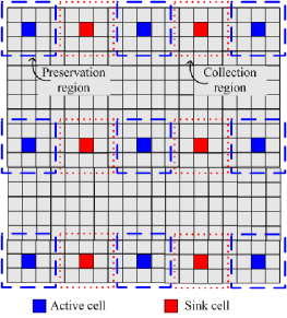
Figure 1: Preservation regions and collection regions.

At the intermediate destination nodes, the received primary packet segments are assembled into the original primary packets. Then in the third subframe, we use the following protocol to deliver the packets to the primary destination nodes:

• Define a collection region as nine primary cells and a layer of secondary cells around them, shown as the square with dotted edges in Fig. 1, where the collection region is located between two preservation regions along the horizontal line and they are not overlapped with each other.

• Deliver the primary packets from the intermediate destination nodes in the secondary tier to the corresponding primary destination nodes in the sink cell, which is defined as the center primary cell of the collection region. The primary destination nodes in the sink cell take turns to receive data by following a TDMA pattern, where the corresponding intermediate destination node in the collection region transmits by pretending as a primary TX node. Given that the third subframe is of an equal length to one primary slot, each primary destination node in the sink cell can receive one primary packet from the corresponding intermediate destination node.

• At each transmission, the intermediate destination node transmits with the same power as that for a primary node, i.e., $Pa_{p}^{\frac{\alpha}{2}}(n)$.

IV Delay and Throughput Analysis for the Secondary Tier

In this section, we discuss the delay and throughput scaling laws for the secondary tier. According to the protocol for the secondary tier, we split the time frame into three equal-length fractions and use one of them for the secondary packet transmissions. Since the above time-sharing strategy only incurs a constant penalty (i.e., 1/3) on the achievable throughput and delay within the secondary tier, the throughput and delay scaling laws are the same as those given in [9], which are summarized by the following theorems.

Theorem 1

With the secondary protocol defined in Section III, the secondary tier can achieve the following throughput per S-D pair and sum throughput w.h.p.:

$$\lambda_{s}(m)=\Theta\left(\frac{1}{m\sqrt{a_{s}(m)}}\right)$$ (4)

and

$$T_{s}(m)=\Theta\left(\frac{1}{\sqrt{a_{s}(m)}}\right),$$ (5)

where $a_{s}(m)\geq 2\log m/m$ and the specific value of $a_{s}(m)$ is determined by $a_{p}(n)$ as shown later in (14).

Theorem 2

With the secondary protocol defined in Section III, the packet delay is given by

$$D_{s}(m)=\Theta\left(\frac{1}{\sqrt{a_{s}(m)}}\right).$$ (6)

Combining the results in (4) and (6), the delay-throughput tradeoff for the secondary tier is given by the following theorem.

Theorem 3

With the secondary protocol defined in Section III, the delay-throughput tradeoff is

$$D_{s}(m)=\Theta(m\lambda_{s}(m)),~{}\textrm{for}~{}\lambda_{s}(m)=O\left(\frac{1}{\sqrt{m\log m}}\right).$$ (7)

For detailed proofs of the above theorems, please refer to [9].

V Delay and Throughput Analysis for the Primary Tier

In this section, we first give the throughput and delay scaling laws for the primary tier, followed by the delay-throughput tradeoff. Due to the page limit, we only show the main results and leave all the proofs to the journal version [10].

V-A Throughput Analysis for the Primary Tier

In order to obtain the throughput scaling law, we first give the following lemmas.

Lemma 1

The numbers of the primary nodes and secondary nodes in each primary cell are $\Theta(na_{p}(n))$ and $\Theta(ma_{p}(n))$ w.h.p., respectively.

Lemma 2

If the secondary nodes compete to be the designated relay nodes for the primary tier by pretending as primary nodes and $a_{p}(n)=o(1)$, a randomly selected designated relay node for the primary packet in each primary cell is a secondary node w.h.p. (due to the fact that $m>n$ and $n\rightarrow\infty$) such that all the primary packets are actually carried over by the secondary tier w.h.p..

Lemma 3

With the protocols given in Section III, an active primary cell can support a constant data rate of $K_{1}$, where $K_{1}>0$ independent of $n$ and $m$.

Lemma 4

With the protocols given in Section III, the secondary tier can deliver the primary packets to the intended primary destination node at a constant data rate of $K_{2}$, where $K_{2}>0$ independent of $n$ and $m$.

Based on Lemmas 1-4, we have the following theorem.

Theorem 4

With the protocols given in Section III, the primary tier can achieve the following throughput per S-D pair and sum throughput w.h.p. when $\beta\geq 2$.

$$\lambda_{p}(n)=\Theta\left(\frac{1}{na_{p}(n)}\right)$$ (8)

and

$$T_{p}(n)=\Theta\left(\frac{1}{a_{p}(n)}\right),$$ (9)

where $a_{p}(n)\geq 2\log n/n$ and $a_{p}(n)=o(1)$.

By setting $a_{p}(n)=2\log n/n$, the primary tier can achieve the following throughput per S-D pair and sum throughput w.h.p.:

$$\lambda_{p}(n)=\Theta\left(\frac{1}{\log n}\right)$$ (10)

and

$$T_{p}(n)=\Theta\left(\frac{n}{\log n}\right).$$ (11)

V-B Delay Analysis of the Primary Tier

We focus on the delay performance of the primary tier with the aid of the secondary tier. In the proposed protocols, we know that the primary tier pours all the primary packets into the secondary tier w.h.p. based on Lemma 2. In order to analyze the delay of the primary tier, we have to calculate the traveling time for the $N$ segments of a primary packet to reach the corresponding intermediate destination node within the secondary tier. Since the S-D paths for the $N$ segments are the same and an active secondary cell (outside all the preservation regions) transmits one packet for each S-D path passing through it within a secondary time slot, we can guarantee that the $N$ segments depart from the $N$ nodes, move hop by hop along the S-D paths, and finally reach the corresponding intermediate destination node in a synchronized fashion. According to the definition of packet delay, the $N$ segments experience the same delay given in (6) within the secondary tier, and all the segments arrive the intermediate destination node within one secondary slot.

Let $L_{p}$ and $L_{s}$ denote the durations of the primary and secondary time slots, respectively. According to the proposed protocols, we have

$$L_{p}=64L_{s}.$$ (12)

Since we split the secondary time frame into three fractions and use one of them for the primary packet transmissions, each primary packet suffers from the following delay

$$D_{p}(n)=\frac{3}{64}D_{s}(m)+C=\Theta\left(\frac{1}{\sqrt{a_{s}(m)}}\right)$$ (13)

where $C$ denotes the average time for a primary packet to travel from the primary source node to the $N$ secondary relay nodes and from the intermediate destination node to the final destination node, which is a constant. We see from (13) that the delay of the primary tier is only determined by the size of the secondary cell $a_{s}(m)$. In order to obtain a better delay performance, we should make $a_{s}(m)$ as large as possible. However, a larger $a_{s}(m)$ results in a decreased throughput per S-D pair in the secondary tier and hence a decreased throughput for the primary tier since all the primary traffic traverses over the secondary tier w.h.p.. In the following, we derive the relationship between $a_{p}(n)$ and $a_{s}(m)$ in our supportive two-tier setup.

We know that given $a_{p}(n)\geq 2\log n/n$, the maximum throughput per S-D pair for the primary tier is $\Theta\left(\frac{1}{na_{p}(n)}\right)$. Since a primary packet is divided into $N$ segments and then routed by $N$ parallel S-D paths within the secondary tier, the supported rate for each secondary S-D pair is required to be $\Theta\left(\frac{1}{Nna_{p}(n)}\right)=\Theta\left(\frac{\sqrt{\log m}}{\sqrt{m}na_{p}(n)}\right)$. As such, based on (4), the corresponding secondary cell size $a_{s}(m)$ needs to be set as

$$a_{s}(m)=\frac{\beta^{2}n^{2}a_{p}^{2}(n)}{2m\log m}$$ (14)

where we have $a_{s}(m)\geq 2\log m/m$ when $a_{p}(n)\geq 2\log n/n$.

Substituting (14) in (13), we have the following theorem.

Theorem 5

According to the proposed protocols in Section III, the primary tier can achieve the following delay w.h.p. when $\beta\geq 2$.

$$D_{p}(n)=\Theta\left(\frac{\sqrt{m\log m}}{na_{p}(n)}\right)=\Theta\left(\frac{\sqrt{n^{\beta}\log n}}{na_{p}(n)}\right).$$ (15)

V-C Delay-throughput Tradeoff for the Primary Tier

Combining the results in (8) and (15), the delay-throughput tradeoff for the primary tier is given by the following theorem.

Theorem 6

With the protocols given in Section III, the delay-throughput tradeoff in the primary tier is given by

$$D_{p}(n)=\Theta\left(\sqrt{n^{\beta}\log n}\lambda_{p}(n)\right)~{}\textrm{for}~{}\lambda_{p}(n)=O\left(\frac{1}{\log n}\right).$$ (16)

VI Conclusion

In this paper, we studied the throughput scaling laws for an interactive two-tier network, where the secondary tier is willing to route packets for the primary tier in an opportunistic fashion. When the secondary tier has a much higher density, with our proposed schemes, the primary tier can achieve a better throughput scaling law of $\Theta\left(1/\log n\right)$ per S-D pair compared to $\Theta\left(1/\sqrt{n\log n}\right)$ in for non-interactive overlaid networks with a different delay-throughput tradeoff.

References

- [1] P. Gupta and P. R. Kumar, “The capacity of wireless networks,” IEEE Trans. Inform. Theory, vol. 46, pp. 388-404, Mar. 2000.
- [2] M. Francheschetti, O. Dousse, D. Tse and P. Thiran, “closing the gap in the capacity of random wireless networks via percolation theory,” IEEE Trans. Inform. Theory, vol. 53, no. 3., pp. 1009-1018, March 2007.
- [3] A. Ozgur, O. Leveque, and D. Tse, “Hierarchical Cooperation Achieves Optimal Capacity Scaling in Ad Hoc Networks,” IEEE Trans. Inform. Theory, vol 53, no. 10, pp. 3549 - 3572, Oct. 2007.
- [4] M. Grossglauser and D. N. C. Tse, “Mobility increases the capacity of ad hoc wireless network,” IEEE/ACM Trans. Networking, vol. 10, no. 4, pp. 477-486, Aug. 2002.
- [5] M. J. Neely and E. Modiano, “Capacity and delay tradeoffs for ad-hoc mobile networks,” IEEE Trans. Inform. Theory, vol. 51, no. 6, pp. 1917-1936, June 2005.
- [6] N. Bansal and Z. Liu, “Capacity, delay and mobility in wireless ad-hoc networks,” IEEE INFOCOM 2003, vol. 2, pp. 1553-1563, Mar. 2003.
- [7] A. E. Gamal, J. Mammen, B. Prabhakar, and D. Shah, “Optimal throughput-delay scaling in wirless networks–part I: the fluid model,” IEEE Trans. Inform. Theory, vol. 52, no. 6, pp. 2568-2592, June 2006.
- [8] S. Jeon, N. Devroye, M. Vu, S. Chung, and V. Tarokh, “Cognitive networks achieve throughput scaling of a homogeneous network,” preprint. Jan. 2008. [Online]. Available: http://arxiv.org/pdf/0801:0938.
- [9] C. Yin, L. Gao, and S. Cui, “Scaling laws for overlaid wireless networks: a cognitive radio network vs. a primary network,” preprint. May 2008. [Online]. Available: http://arxiv.org/pdf/0805:1209.
- [10] L. Gao, R. Zhang, C. Yin, and S. Cui, “Delay-throughput tradeoff for supportive two-tier networks,” in preparation.