Fracture Toughness and Maximum Stress
in a Disordered Lattice System

Abstract

Fracture in a disordered lattice system is studied. In our system, particles are initially arranged on the triangular lattice and each nearest-neighbor pair is connected with a randomly chosen soft or hard Hookean spring. Every spring has the common threshold of stress at which it is cut. We make an initial crack and expand the system perpendicularly to the crack. We find that the maximum stress in the stress-strain curve is larger than those in the systems with soft or hard springs only (uniform systems). Energy required to advance fracture is also larger in some disordered systems, which indicates that the fracture toughness improves. The increase of the energy is caused by the following two factors. One is that the soft spring is able to hold larger energy than the hard one. The other is that the number of cut springs increases as the fracture surface becomes tortuous in disordered systems.

I Introduction

Composite of hard and soft materials sometimes results in increase of toughness. An example is double-network (DN) gel that is an interpenetrating network of brittle polyelectrolyte gel and flexible polymer chains. A DN gel can have much higher toughness than ordinary gels Gong et al. (2003); Na et al. (2004); Tanaka et al. (2005a, b); Tanaka (2007). The second example is nacre, which has a layered structure of brittle ceramic and soft organic matrix. The toughness of nacre is comparable to that of some high-technology structural ceramicsCurrey (1977); Jackson et al. (1988). In addition, the toughness of brittle $\mathrm{Al_{2}O_{3}}$ ceramics is known to be increased through the incorporation of metals like tungsten, copper or nickel. The bending strength also increases with the content of these metalsTuan and Brook (1990); Sekino and Niihara (1997); Oh et al. (1998); Li et al. (2004).

These materials have been studied as follows. TanakaTanaka (2007) argued that DN gel locally softens and the crack extends within the softened zone. He estimated effective fracture energy, whose order of magnitude is consistent with experiments. With respect to nacre, it is considered that a weak material reduces drastically the stress concentration near the fracture tipsde Gennes and Okumura (2000) and the maximum stress increases with the repeat period of structure. Okumura examined a double elastic network of hard and soft materials and derived toughness enhancement factorsOkumura (2004), where the ratio of the two elastic moduli and the mesh size as well as the volume fraction of each element are especially important in controlling toughness. For the composites of $\mathrm{Al_{2}O_{3}}$, Ashby, Blunt and Bannister emphasize that the inclusions bridge the crack and are stretched as the crack opens, leading to enhancement of toughnessAshby et al. (1989). They executed experiments of bonding a wire into a thick-wall glass capillary and showed that the toughness increases with the diameter of wires. It has been derived that the toughness is proportional to the square root of the product of volume fraction and inclusion size, which is confirmed in experiments by Tuan and BrookTuan and Brook (1990).

Although structure of the composite materials may be important in the above examples, we here focus on whether toughness can be improved only by mixing hard and soft materials. Specifically, we consider a model system which consists of particles initially on the triangular lattice. Every nearest-neighbor pair of the particles is connected with a randomly chosen hard or soft spring except those on the initial crack. Each spring is assumed to break if it is subject to stress larger than a threshold value, which is common to all springs. We numerically investigate behavior of the system when it is stretched at constant velocity and find that the system can hold up larger stress than a uniform system with only a kind of spring can. Moreover, the maximum stress depends on the fraction of soft springs and the ratio of the spring constants, respectively.

There are some related works in the literatureBeale and Srolovitz (1988); nol et al. (1996); Politi and Zei (2001). In particular, Beale and Srolovitz studied the system where springs are present with a probabilityBeale and Srolovitz (1988). They obtained analytically the distribution function of the initial failure stress and verified it using computer simulation. Espanõl, Zúñiga and Rubio showed numerically that the stress of the most stretched spring is represented by a function of the initial notch lengthnol et al. (1996). To our knowledge, however, enhancement of the maximum stress or toughness in such a disordered system has not been reported to date.

We organize the paper as follows. In the next section, our model and simulation method are described. Then we show our numerical results in Sec. III. The last section is devoted to summary and discussion.

II Model and Simulation

Our model system consists of $2525$ particles initially on the triangular lattice arranged in $51$ columns each of which has alternatingly $49$ or $50$ particles. The particles have the same mass and each pair of nearest-neighbor particles is connected by a linear spring of natural length $l_{0}$, which is equal to the lattice spacing. Spring constant $k_{1}$ or $k_{2}$ ($k_{1}\geq k_{2}$) is randomly assigned to each spring according to a given ratio $1-r:r$. Namely, $r$ denotes the fraction of soft springs. Each spring is assumed to break if the force on the spring exceeds a threshold value $\sigma^{*}$, which is common to all springs. The broken springs do not generate any elastic force. As shown in Fig. 1, twenty springs from the top between the $24$th and the $25$th columns of particles are cut in the initial condition. Thus, the initial crack is about $1/5$ as long as the column length. The particles on the leftmost (or rightmost) column move as one object, and we call them walls (Fig. 2). The walls are moved by an external force in the outward directions at constant velocity $v_{s}$ as shown in Fig. 3. The walls are assumed to be vertically incompressible. Moreover, the viscous force with viscosity coefficient $\eta$ acts on the particles. We assume that $v_{s}$ is slow and the viscous force is strong enough to make the dynamics of particles overdamped. Thus, the motion of the $i$th particle obeys the following equation,

$$\sum_{j}k_{ij}\left(\left|\mathbf{x}_{i}-\mathbf{x}_{j}\right|-l_{0}\right)\hat{\mathbf{x}}_{j\to i}+\eta\dot{\mathbf{x}}_{i}=0,$$ (1)

where $\mathbf{x}_{i}$ denotes the position of the $i$th particle, $k_{ij}$ is the spring constant of the spring between the $i$th and $j$th particles, and $\hat{\mathbf{x}}_{j\to i}$ is the unit vector from the $j$th particle to the $i$th one. The summation runs over the nearest neighbors of the $i$th particle.

Because length and time can be rescaled with the natural length $l_{0}$ and $\eta/k_{2}$, respectively, we can set $l_{0}=1$ and $\eta/k_{2}=1$ without loss of generality. We further assume that $\sigma^{*}=1$ for simplicity. Then the remaining system parameters are $k=k_{1}/k_{2}>1$, $r$ and $v_{s}$. We call $k$ the elastic modulus ratio in this paper.

Simulations are basically carried out using the fourth-order Runge-Kutta method with the time step $\Delta t=1.0\times 10^{-2}$. However, the time step is changed temporally when a spring breaks as follows. If the computed force of a spring, $\sigma^{\prime}$, which is below the threshold $\sigma^{*}$ at time $t_{0}$ exceeds $\sigma^{*}$ until $t_{0}+\Delta t$, we approximate the change of force between time $t_{0}$ and $t_{0}+\Delta t$ by a linear function and obtain the new time step $\delta t$ determined by $\sigma^{\prime}(t_{0}+\delta t)=\sigma^{*}$. That is,

$$\delta t=\frac{\sigma^{*}-\sigma^{\prime}(t_{0})}{\sigma^{\prime}(t_{0}+\Delta t)-\sigma^{\prime}(t_{0})}\Delta t.$$

After the motion of the particles between $t_{0}$ and $t_{0}+\delta t$ are calculated again using the fourth-order Runge-Kutta method, the spring is cut. Then, the next step proceeds with the normal time step $\Delta t$.

We compute stress $\sigma$ and strain $\varepsilon$ in the horizontal direction at the walls as

$$\sigma = \frac{1}{H_{0}}\sum_{i=1}^{N_{w}}\sum_{j}k_{ij}\left(\mid\mathbf{x}_{i}-\mathbf{x}_{j}\mid-l_{0}\right)\frac{\mid x_{j}-x_{i}\mid}{\mid\mathbf{x}_{j}-\mathbf{x}_{i}\mid},$$ (2)

$$\varepsilon = \frac{\mid X_{r}(t)-X_{l}(t)\mid-W_{0}}{W_{0}},$$ (3)

where $N_{w}$ is the number of particles on each wall, $x_{k}$ is the horizontal coordinate of the $k$th particle, $X_{l}$ and $X_{r}$ denote the horizontal coordinates of the left and right walls, and $H_{0}$ and $W_{0}$ are the height of the walls and the distance between the walls at the initial time, respectively. The summation for $i$ is taken over the particles on the wall, and $j$ runs over the nearest-neighbors of each $i$. Since the values of stress evaluated at the left and right walls are almost the same, we do not distinguish them in the following.

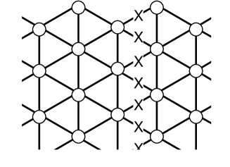
Figure 1: Upper 20 springs between the $24$th and the $25$th columns are initially cut.

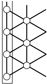
Figure 2: The particles on a wall move as one object.

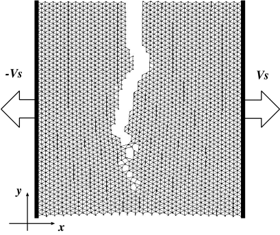
Figure 3: Crack propagates as the walls are moved outward in the horizontal direction. The initial crack is introduced in the upper part of the system.

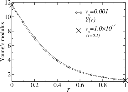
Figure 4: Young’s modulus vs the fraction of soft springs $r$. Dotted line represents the theoretical estimate by Garboczi and Thorpe.

Young’s modulus of our system was calculated by Garboczi and ThorpeFeng et al. (1985); Garboczi and Thorpe (1986) by applying the effective medium theory. It is a kind of mean-field theory which approximates the random and disordered system with an equivalent uniform system. The spring constant $k^{*}$ of the uniform system corresponding to our system is determined by the relation

$$\frac{2(1-r)(k^{*}-k_{1})}{k^{*}+2k_{1}}+\frac{2r(k^{*}-k_{2})}{k^{*}+k_{2}}=0.$$

Thus, the Young’s modulus $Y$ is obtained as

$$Y=\frac{1}{\sqrt{3}}\left(-b+\sqrt{b^{2}+8k}\right)$$

where $b=(k-1)(3r-1)+1$. Because the number of soft springs increases with $r$, $Y$ is a decreasing function of $r$. Fig. 4 shows a very good agreement between the theory and our numerical results. The latter is computed from the initial slope of the stress-strain (S-S) curve. We remark that the system with vertically compressible walls and no initial cracks is used for the computation. The small deviation is considered as due to the finiteness of the wall velocity $v_{s}=10^{-3}$, since the agreement gets much better when a smaller velocity $v_{s}=10^{-7}$ is used. In addition, the Poisson’s ratio $\gamma$ is theoretically computed to be $1/3$, while $\gamma$ lies between $0.29$ and $0.33$ numerically when $v_{s}=10^{-3}$.

III Results

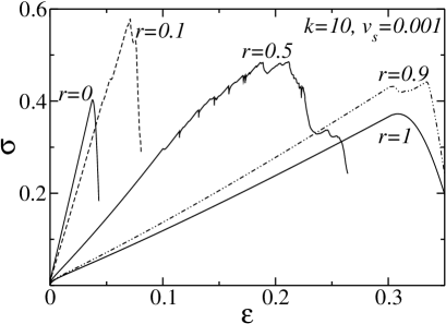
Figure 5: Stress-strain curve for the systems with various $r$ and fixed $k=10$.

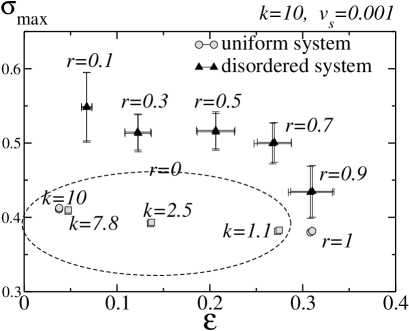
Figure 6: The average of the maximum stress for the disordered systems with $k=10$ (circles and solid triangles) and those for the uniform systems with various $k$ (squares).

In Fig. 5, we show the S-S curves obtained for the models with various $r$ and fixed $k$ at $10$. Stress $\sigma$ initially increases linearly with strain $\varepsilon$. When the stress reaches a maximum, the crack begins to propagate. The value of the maximum stress varies from sample to sample in the disordered cases ($0<r<1$). However, for almost all samples, the maximum stress is larger than those at $r=0$ and $r=1$ despite the fact that the threshold $\sigma^{*}$ is common to the soft and hard springs. Thus, as shown in Fig. 6, the average values of the maximum stress exhibit significant enhancement compared with the uniform cases. We note that this is entirely a nonlinear effect. Linear properties like Young’s modulus and Poisson’s ratio are explained by considering equivalent uniform systems, which show no increase of the maximum stress. Squares in Fig. 6 represent the maximum stress for uniform models with $r=0$ and $k=1.1,2.5,7.8$, whose Young’s modulus correspond to $k=10$ and $r=0.9,0.5,0.1$, respectively.

We consider that this increase of the maximum stress should be connected with differences between the stress distributions in the disordered systems and that in the uniform systems. Figs. 7 and 8 illustrate the $x$ component of each spring force $\sigma^{\prime}_{x}$ against the distance between the spring and the crack tip in the uniform system (Fig. 7) and in the disordered system (Fig. 8). The value of $\sigma$ is the same in the both figures. In the former case, the forces are large only near the crack tip, and for $d>10$ most values of the forces are distributed around $0.3$ or $0$. Contrastingly, in the latter case, there are many springs with forces beyond $0.3$ in the range $d>10$. Thus, many springs distant from the crack tip suffer larger stress in the disordered system than in the uniform system. It is more evident in Fig. 9 which shows the distribution of the forces on the springs initially inclined $\pm 30^{\circ}$ to the horizontal axis. We find there that more springs share larger stress in the disordered system, which makes stress concentration at the crack tip to be eased.

In our simulation, the lattice structure remains unchanged. We notice concentration of data near the horizontal axis in Figs. 7 and 8. They represent that the initially vertical springs do not change their orientations and do not contribute to the stress, which is true even near the crack tip. The other springs also keep their orientations. The inset in Fig. 9 shows the distribution of angle displacements to the horizontal direction for the springs initially $\pm 30^{\circ}$ inclined to the $x$ axis. The distribution is a little moved to the horizontal direction and widened, but not so much. This means that the lattice is only slightly deformed as the system is stretched. This is due to the relatively small value of the threshold $\sigma^{*}=1$. Because of the smallness of the parameter, the fracture starts to expand at small strain $\varepsilon\cong 0.05$ for $r=0.1$. At this value of strain, deformation of the lattice is very small.

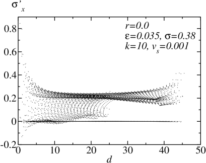
Figure 7: Spatial distribution of the $x$ components of spring forces, $\sigma^{\prime}_{x}$, in the uniform system with $r=0$ when strain $\varepsilon=0.035$ and stress $\sigma=0.38$.

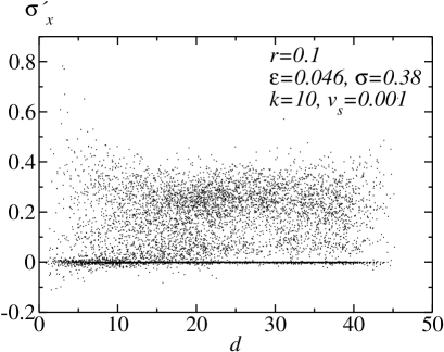
Figure 8: Same as Fig. 7 except in a sample of the disordered system with $r=0.1$ when strain $\varepsilon=0.046$ and stress $\sigma=0.38$.

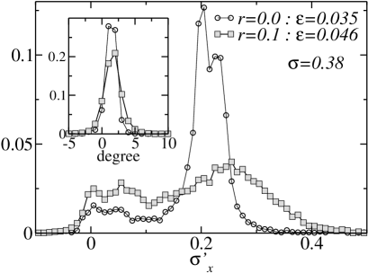
Figure 9: Distribution of the force $\sigma^{\prime}$ for the springs initially inclined $\pm 30^{\circ}$ to the $x$-axis. Inset: Distribution of angle displacements to the horizontal direction for the springs. The stress value $\sigma=0.38$ is the same as Figs. 7 and 8.

Not only the maximum stress but also the toughness of the system improves in the disordered system. The toughness is defined as the work required to make a unit area of fracture surface in quasi-static fracture. We identify the work with the injected energy to the system during advancing of cracks, $E_{s}$, which is defined by

$$E_{s}=H_{0}W_{0}A\varepsilon,$$ (4)

where $A$ represents the area under the S-S curve. Though the estimate contains other dissipative effects, they are expected to be small. We assume further that the crack lengths do not vary with $r$. The upper line in Fig. 10 shows $E_{s}$ averaged over $30$ samples, which indicates that the toughness drastically increases with $r$ in region $0<r<0.4$. In addition, the toughness in $0.4<r<1$ is larger than those of the uniform systems ($r=0$ or $r=1$).

A part of the injected energy is released by the fracture. The released energy $E_{r}$ also changes with $r$ as shown in Fig. 10. It increases with the ratio of soft springs $r$ except around $r=0.5$. This is partly because a soft spring releases larger energy than a hard one in our model; The spring with spring constant $k$ releases energy ${\sigma^{*}}^{2}/2k$. In addition, increase in the number of cut springs also raises $E_{r}$. A hard spring is easily cut by smaller strain than a soft spring. Thus, the crack tip proceeds with avoiding soft springs. As the result, the crack meanders in the disordered systems, while it goes straight in the uniform systems. The meandering causes the increase in the number of cut springs, $N_{cut}$. We numerically observe that $N_{cut}$ has the maximum near $r=0.4$ as shown in Fig. 11. The inflection of $E_{r}$ around $r=0.5$ is due to the competition of the two factors: the increase of soft springs which pushes up $E_{r}$ and the decrease of $N_{cut}$. Precise relation between $E_{s}$ and $E_{r}$ is unknown, but they largely exhibit similar change with $r$. Fig. 12 shows that the ratio $E_{s}/E_{r}$ does not change with $r$ very much. Thus, the increase of $E_{r}$ in the disordered systems also brings the increase of $E_{s}$, namely the increase of toughness.

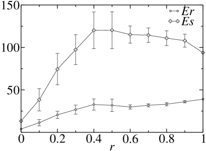
Figure 10: The injected energy $E_{s}$ and the released energy $E_{r}$ for several $r$

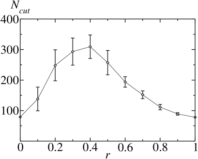
Figure 11: Number of cut springs for several $r$.

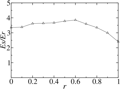
Figure 12: $Es/E_{r}$ vs $r$.

IV Conclusion and Discussion

Through investigations of fracture in the disordered lattice systems with unequal spring constants, we have found that both of the maximum stress and the toughness improve in the disordered systems. Because a soft spring holds larger energy than a hard one, and because presence of soft springs makes fracture meander, the released energy $E_{r}$ becomes larger in the disordered systems than the uniform ones. This leads to the improvement of the toughness.

Although we have so far fixed the ratio of the spring constants $k$ in the simulations, improvement of maximum stress and fracture toughness is observed in a wide range of $k$ in our preliminary computation. Fig. 13 shows the maximum stress $\sigma_{\mathrm{max}}$ for disordered systems with various $k$ and fixed $r$ at $0.1$. Compared to the data for $r=0$ in Fig. 6, we realize that the increase of the maximum stress is seen unless $k$ is too large. Moreover, $\sigma_{\mathrm{max}}$ increases with $k$ in the range $1\leq k\leq 10$ and decreases for $k>10$. For $k$ close to $1$, $\sigma_{\mathrm{max}}$ is small because the system becomes nearly uniform. In contrast, if $k$ is too large, small strain causes large tension for hard springs but little effects on soft springs. Therefore, most stress is sustained by hard springs only, and soft springs are not effective. It means that the system behaves like diluted ones where $\sigma_{\mathrm{max}}$ becomes small. We also observe that energy $E_{s}$ takes the maximum value at some $0<r<1$ if $k$ is distinctly larger than $1$. Details of the computation will be reported elsewhere.

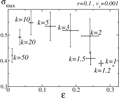
Figure 13: The maximum stress for several $k$ at $r=0.1$. Each point is obtained from averaging over 30 samples.

Although the soft and hard springs are cut at the same stress value in our models, this condition can be modified. Let us consider the case where the springs are cut at the same elastic energy $e^{*}$. Then, we again find that the toughness improves in the disordered system for $r=0.1$, $k=10$, and $e^{*}=5$; For $r=0.0,0.1$, the average $E_{s}=696$ and $941$, $E_{r}=390$ and $420$, respectively. Because the released energy when a spring is cut is common for all springs, $E_{r}$ is proportional to the number of cut springs, $N_{cut}$. Accordingly, the improvement of toughness in the disordered systems is caused as the result of meandering crack. The maximum stress also increases in some samples as shown in Fig. 14. However, their average represented by a circle point does not show a clear improvement. We consider that the maximum stress should depend on $r$, and detailed study of its dependence is planned for the future.

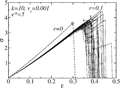
Figure 14: S-S curves for the uniform system ($r=0$) and the disordered system ($r=0.1,k=10$) where every spring breaks if its elastic energy exceeds a value $e^{*}$.

The fracture phenomenon naturally depends on the threshold stress $\sigma^{*}$. It may drastically change with $\sigma^{*}$. Our choice that $\sigma^{*}=1$ is rather small, and fractures can expand with small strain below $0.3$. Thus, we have observed fractures without large deformation of the arrangement of the triangular lattice. However, for materials like polymer gels, fractures occur when the material suffers large deformation. It is interesting to study if such large deformation can improve the maximum stress or the toughness of the materials.

Our system is not large enough to be macroscopic. We have checked that the system of doubled size $101\times 100$ shows almost the same results. However, it still may not be sufficient to restore isotropy. Thus, the orientation of the lattice may also have influences on the fracture. For example, if we use the system rotated by $90^{\circ}$, all spring forces have components parallel to the external force. Thus, the maximum stress can change from our model where the vertical springs do not contribute to the improvement of the toughness. If we want to obtain results independent of orientation of the system, use of random lattices will be effective because we can expect that isotropy is restored in systems as large as our model. It is a future problem to investigate such a system.

Our findings may be applied to design some new material with high fracture toughness. However, our model is two dimensional and too simple to apply real fractures. Some extensions, for example, to three dimensions or to realistic interactions are future problems.