Kronecker graphs: An Approach to Modeling Networks

Abstract

How can we generate realistic networks? In addition, how can we do so with a mathematically tractable model that allows for rigorous analysis of network properties? Real networks exhibit a long list of surprising properties: Heavy tails for the in- and out-degree distribution, heavy tails for the eigenvalues and eigenvectors, small diameters, and densification and shrinking diameters over time. Current network models and generators either fail to match several of the above properties, are complicated to analyze mathematically, or both. Here we propose a generative model for networks that is both mathematically tractable and can generate networks that have all the above mentioned structural properties. Our main idea here is to use a non-standard matrix operation, the Kronecker product, to generate graphs which we refer to as “Kronecker graphs”.

First, we show that Kronecker graphs naturally obey common network properties. In fact, we rigorously prove that they do so. We also provide empirical evidence showing that Kronecker graphs can effectively model the structure of real networks.

We then present KronFit, a fast and scalable algorithm for fitting the Kronecker graph generation model to large real networks. A naive approach to fitting would take super-exponential time. In contrast, KronFit takes linear time, by exploiting the structure of Kronecker matrix multiplication and by using statistical simulation techniques.

Experiments on a wide range of large real and synthetic networks show that KronFit finds accurate parameters that very well mimic the properties of target networks. In fact, using just four parameters we can accurately model several aspects of global network structure. Once fitted, the model parameters can be used to gain insights about the network structure, and the resulting synthetic graphs can be used for null-models, anonymization, extrapolations, and graph summarization.

Keywords: Kronecker graphs, Network analysis, Network models, Social networks, Graph generators, Graph mining, Network evolution

1 Introduction

What do real graphs look like? How do they evolve over time? How can we generate synthetic, but realistic looking, time-evolving graphs? Recently, network analysis has been attracting much interest, with an emphasis on finding patterns and abnormalities in social networks, computer networks, e-mail interactions, gene regulatory networks, and many more. Most of the work focuses on static snapshots of graphs, where fascinating “laws” have been discovered, including small diameters and heavy-tailed degree distributions.

In parallel with discoveries of such structural “laws” there has been effort to find mechanisms and models of network formation that generate networks with such structures. So, a good realistic network generation model is important for at least two reasons. The first is that it can generate graphs for extrapolations, hypothesis testing, “what-if” scenarios, and simulations, when real graphs are difficult or impossible to collect. For example, how well will a given protocol run on the Internet five years from now? Accurate network models can produce more realistic models for the future Internet, on which simulations can be run. The second reason is more subtle. It forces us to think about network properties that generative models should obey to be realistic.

In this paper we introduce Kronecker graphs, a generative network model which obeys all the main static network patterns that have appeared in the literature Faloutsos et al. (1999); Albert et al. (1999); Chakrabarti et al. (2004); Farkas et al. (2001); Mihail and Papadimitriou (2002); Watts and Strogatz (1998). Our model also obeys recently discovered temporal evolution patterns Leskovec et al. (2005b, 2007a). And, contrary to other models that match this combination of network properties (as for example, Bu and Towsley (2002); Klemm and Eguíluz (2002); Vázquez (2003); Leskovec et al. (2005b); Zheleva et al. (2009)), Kronecker graphs also lead to tractable analysis and rigorous proofs. Furthermore, the Kronecker graphs generative process also has a nice natural interpretation and justification.

Our model is based on a matrix operation, the Kronecker product. There are several known theorems on Kronecker products. They correspond exactly to a significant portion of what we want to prove: heavy-tailed distributions for in-degree, out-degree, eigenvalues, and eigenvectors. We also demonstrate how a Kronecker graphs can match the behavior of several real networks (social networks, citations, web, internet, and others). While Kronecker products have been studied by the algebraic combinatorics community (see, e.g., Chow (1997); Imrich (1998); Imrich and Klavžar (2000); Hammack (2009)), the present work is the first to employ this operation in the design of network models to match real data.

Then we also make a step further and tackle the following problem: Given a large real network, we want to generate a synthetic graph, so that the resulting synthetic graph matches the properties of the real network as well as possible.

Ideally we would like: (a) A graph generation model that naturally produces networks where many properties that are also found in real networks naturally emerge. (b) The model parameter estimation should be fast and scalable, so that we can handle networks with millions of nodes. (c) The resulting set of parameters should generate realistic-looking networks that match the statistical properties of the target, real networks.

In general the problem of modeling network structure presents several conceptual and engineering challenges: Which generative model should we choose, among the many in the literature? How do we measure the goodness of the fit? (Least squares don’t work well for power laws, for subtle reasons!) If we use likelihood, how do we estimate it faster than in time quadratic on the number of nodes? How do we solve the node correspondence problem, i.e., which node of the real network corresponds to what node of the synthetic one?

To answer the above questions we present KronFit, a fast and scalable algorithm for fitting Kronecker graphs by using the maximum likelihood principle. When calculating the likelihood there are two challenges: First, one needs to solve the node correspondence problem by matching the nodes of the real and the synthetic network. Essentially, one has to consider all mappings of nodes of the network to the rows and columns of the graph adjacency matrix. This becomes intractable for graphs with more than tens of nodes. Even when given the “true” node correspondences, just evaluating the likelihood is still prohibitively expensive for large graphs that we consider, as one needs to evaluate the probability of each possible edge. We present solutions to both of these problems: We develop a Metropolis sampling algorithm for sampling node correspondences, and approximate the likelihood to obtain a linear time algorithm for Kronecker graph model parameter estimation that scales to large networks with millions of nodes and edges. KronFit gives orders of magnitude speed-ups against older methods (20 minutes on a commodity PC, versus 2 days on a 50-machine cluster).

Our extensive experiments on synthetic and real networks show that Kronecker graphs  can efficiently model statistical properties of networks, like degree distribution and diameter, while using only four parameters.

Once the model is fitted to the real network, there are several benefits and applications:

1. Network structure: the parameters give us insight into the global structure of the network itself.

2. Null-model: when working with network data we would often like to assess the significance or the extent to which a certain network property is expressed. We can use Kronecker graph as an accurate null-model.

3. Simulations: given an algorithm working on a graph we would like to evaluate how its performance depends on various properties of the network. Using our model one can generate graphs that exhibit various combinations of such properties, and then evaluate the algorithm.

4. Extrapolations: we can use the model to generate a larger graph, to help us understand how the network will look like in the future.

5. Sampling: conversely, we can also generate a smaller graph, which may be useful for running simulation experiments (e.g., simulating routing algorithms in computer networks, or virus/worm propagation algorithms), when these algorithms may be too slow to run on large graphs.

6. Graph similarity: to compare the similarity of the structure of different networks (even of different sizes) one can use the differences in estimated parameters as a similarity measure.

7. Graph visualization and compression: we can compress the graph, by storing just the model parameters, and the deviations between the real and the synthetic graph. Similarly, for visualization purposes one can use the structure of the parameter matrix to visualize the backbone of the network, and then display the edges that deviate from the backbone structure.

8. Anonymization: suppose that the real graph cannot be publicized, like, e.g., corporate e-mail network or customer-product sales in a recommendation system. Yet, we would like to share our network. Our work gives ways to such a realistic, ’similar’ network.

The current paper builds on our previous work on Kronecker graphs Leskovec et al. (2005a); Leskovec and Faloutsos (2007) and is organized as follows: Section 2 briefly surveys the related literature. In section 3 we introduce the Kronecker graph model, and give formal statements about the properties of networks it generates. We investigate the model using simulation in Section 4 and continue by introducing KronFit, the Kronecker graphs parameter estimation algorithm, in Section  5. We present experimental results on a wide range of real and synthetic networks in Section 6. We close with discussion and conclusions in sections 7 and 8.

2 Relation to previous work on network modeling

Networks across a wide range of domains present surprising regularities, such as power laws, small diameters, communities, and so on. We use these patterns as sanity checks, that is, our synthetic graphs should match those properties of the real target graph.

Most of the related work in this field has concentrated on two aspects: properties and patterns found in real-world networks, and then ways to find models to build understanding about the emergence of these properties. First, we will discuss the commonly found patterns in (static and temporally evolving) graphs, and finally, the state of the art in graph generation methods.

2.1 Graph Patterns

Here we briefly introduce the network patterns (also referred to as properties or statistics) that we will later use to compare the similarity between the real networks and their synthetic counterparts produced by the Kronecker graphs model. While many patterns have been discovered, two of the principal ones are heavy-tailed degree distributions and small diameters.

Degree distribution: The degree-distribution of a graph is a power law if the number of nodes $N_{d}$ with degree $d$ is given by $N_{d}\propto d^{-\gamma}\quad(\gamma>0)$ where $\gamma$ is called the power law exponent. Power laws have been found in the Internet Faloutsos et al. (1999), the Web Kleinberg et al. (1999); Broder et al. (2000), citation graphs Redner (1998), online social networks Chakrabarti et al. (2004) and many others.

Small diameter: Most real-world graphs exhibit relatively small diameter (the “small- world” phenomenon, or “six degrees of separation” Milgram (1967)): A graph has diameter $D$ if every pair of nodes can be connected by a path of length at most $D$ edges. The diameter $D$ is susceptible to outliers. Thus, a more robust measure of the pair wise distances between nodes in a graph is the integer effective diameter Tauro et al. (2001), which is the minimum number of links (steps/hops) in which some fraction (or quantile $q$, say $q=0.9$) of all connected pairs of nodes can reach each other. Here we make use of effective diameter which we define as follows Leskovec et al. (2005b). For each natural number $h$, let $g(h)$ denote the fraction of connected node pairs whose shortest connecting path has length at most $h$, i.e., at most $h$ hops away. We then consider a function defined over all positive real numbers $x$ by linearly interpolating between the points $(h,g(h))$ and $(h+1,g(h+1))$ for each $x$, where $h=\lfloor x\rfloor$, and we define the effective diameter of the network to be the value $x$ at which the function $g(x)$ achieves the value 0.9. The effective diameter has been found to be small for large real-world graphs, like Internet, Web, and online social networks Albert and Barabási (2002); Milgram (1967); Leskovec et al. (2005b).

Hop-plot: It extends the notion of diameter by plotting the number of reachable pairs $g(h)$ within $h$ hops, as a function of the number of hops $h$ Palmer et al. (2002). It gives us a sense of how quickly nodes’ neighborhoods expand with the number of hops.

Scree plot: This is a plot of the eigenvalues (or singular values) of the graph adjacency matrix, versus their rank, using the logarithmic scale. The scree plot is also often found to approximately obey a power law Chakrabarti et al. (2004); Farkas et al. (2001). Moreover, this pattern was also found analytically for random power law graphs Mihail and Papadimitriou (2002); Chung et al. (2003).

Network values: The distribution of eigenvector components (indicators of “network value”) associated to the largest eigenvalue of the graph adjacency matrix has also been found to be skewed Chakrabarti et al. (2004).

Node triangle participation: Edges in real-world networks and especially in social networks tend to cluster Watts and Strogatz (1998) and form triads of connected nodes. Node triangle participation is a measure of transitivity in networks. It counts the number of triangles a node participates in, i.e., the number of connections between the neighbors of a node. The plot of the number of triangles $\Delta$ versus the number of nodes that participate in $\Delta$ triangles has also been found to be skewed Tsourakakis (2008).

Densification power law: The relation between the number of edges $E(t)$ and the number of nodes $N(t)$ in evolving network at time $t$ obeys the densification power law (DPL), which states that $E(t)\propto N(t)^{a}$. The densification exponent $a$ is typically greater than $1$, implying that the average degree of a node in the network is increasing over time (as the network gains more nodes and edges). This means that real networks tend to sprout many more edges than nodes, and thus densify as they grow Leskovec et al. (2005b, 2007a).

Shrinking diameter: The effective diameter of graphs tends to shrink or stabilize as the number of nodes in a network grows over time Leskovec et al. (2005b, 2007a). This is somewhat counterintuitive since from common experience as one would expect that as the volume of the object (a graph) grows, the size (i.e., the diameter) would also grow. But for real networks this does not hold as the diameter shrinks and then seems to stabilize as the network grows.

2.2 Generative models of network structure

The earliest probabilistic generative model for graphs was the Erdős-Rényi Erdős and Rényi (1960) random graph model, where each pair of nodes has an identical, independent probability of being joined by an edge. The study of this model has led to a rich mathematical theory. However, as the model was not developed to model real-world networks it produces graphs that fail to match real networks in a number of respects (for example, it does not produce heavy-tailed degree distributions).

The vast majority of recent network models involve some form of preferential attachment Barabási and Albert (1999); Albert and Barabási (2002); Winick and Jamin (2002); Kleinberg et al. (1999); Kumar et al. (1999); Flaxman et al. (2007) that employs a simple rule: new node joins the graph at each time step, and then creates a connection to an existing node $u$ with the probability proportional to the degree of the node $u$. This leads to the “rich get richer” phenomena and to power law tails in degree distribution. However, the diameter in this model grows slowly with the number of nodes $N$, which violates the “shrinking diameter” property mentioned above.

There are also many variations of preferential attachment model, all somehow employing the “rich get richer” type mechanism, e.g., the “copying model” Kumar et al. (2000), the “winner does not take all” model Pennock et al. (2002), the “forest fire” model Leskovec et al. (2005b), the “random surfer model” Blum et al. (2006), etc.

A different family of network methods strives for small diameter and local clustering in networks. Examples of such models include the small-world model Watts and Strogatz (1998) and the Waxman generator Waxman (1988). Another family of models shows that heavy tails emerge if nodes try to optimize their connectivity under resource constraints Carlson and Doyle (1999); Fabrikant et al. (2002).

In summary, most current models focus on modeling only one (static) network property, and neglect the others. In addition, it is usually hard to analytically analyze properties of the network model. On the other hand, the Kronecker graph model we describe in the next section addresses these issues as it matches multiple properties of real networks at the same time, while being analytically tractable and lending itself to rigorous analysis.

2.3 Parameter estimation of network models

Until recently relatively little effort was made to fit the above network models to real data. One of the difficulties is that most of the above models usually define a mechanism or a principle by which a network is constructed, and thus parameter estimation is either trivial or almost impossible.

Most work in estimating network models comes from the area of social sciences, statistics and social network analysis where the exponential random graphs, also known as $p*$ model, were introduced Wasserman and Pattison (1996). The model essentially defines a log linear model over all possible graphs $G$, $p(G|\theta)\propto\exp(\theta^{T}s(G))$, where $G$ is a graph, and $s$ is a set of functions, that can be viewed as summary statistics for the structural features of the network. The $p*$ model usually focuses on “local” structural features of networks (like, e.g., characteristics of nodes that determine a presence of an edge, link reciprocity, etc.). As exponential random graphs have been very useful for modeling small networks, and individual nodes and edges, our goal here is different in a sense that we aim to accurately model the structure of the network as a whole. Moreover, we aim to model and estimate parameters of networks with millions of nodes, while even for graphs of small size ($>100$ nodes) the number of model parameters in exponential random graphs usually becomes too large, and estimation prohibitively expensive, both in terms of computational time and memory.

Regardless of a particular choice of a network model, a common theme when estimating the likelihood $P(G)$ of a graph $G$ under some model is the challenge of finding the correspondence between the nodes of the true network and its synthetic counterpart. The node correspondence problem results in the factorially many possible matchings of nodes. One can think of the correspondence problem as a test of graph isomorphism. Two isomorphic graphs $G$ and $G^{\prime}$ with differently assigned node IDs should have same likelihood $P(G)=P(G^{\prime})$ so we aim to find an accurate mapping between the nodes of the two graphs.

An ordering or a permutation defines the mapping of nodes in one network to nodes in the other network. For example, Butts Butts (2005) used permutation sampling to determine similarity between two graph adjacency matrices, while Bezáková et al. Bezáková et al. (2006) used permutations for graph model selection. Recently, an approach for estimating parameters of the “copying” model was introduced Wiuf et al. (2006), however authors also note that the class of “copying” models may not be rich enough to accurately model real networks. As we show later, Kronecker graph model seems to have the necessary expressive power to mimic real networks well.

3 Kronecker graph model

The Kronecker graph model we propose here is based on a recursive construction. Defining the recursion properly is somewhat subtle, as a number of standard, related graph construction methods fail to produce graphs that densify according to the patterns observed in real networks, and they also produce graphs whose diameters increase. To produce densifying graphs with constant/shrinking diameter, and thereby match the qualitative behavior of a real network, we develop a procedure that is best described in terms of the Kronecker product of matrices.

Symbol	Description
${G}$	Real network
$N$	Number of nodes in ${G}$
$E$	Number of edges in ${G}$
${K}$	Kronecker graph (synthetic estimate of $G$)
${{K}}_{1}$	Initiator of a Kronecker graphs
${N}_{1}$	Number of nodes in initiator ${{K}}_{1}$
${E}_{1}$	Number of edges in ${{K}}_{1}$ (the expected number of edges in ${\cal P}_{1}$, ${E}_{1}=\sum{\theta_{{ij}}}$)
$G\otimes H$	Kronecker product of adjacency matrices of graphs $G$ and $H$
${{K}}_{1}^{[k]}={{K}}_{k}=K$	$k^{th}$ Kronecker power of ${{K}}_{1}$
${{K}}_{1}[i,j]$	Entry at row $i$ and column $j$ of ${{K}}_{1}$
${\Theta}={\cal P}_{1}$	Stochastic Kronecker initiator
${\cal P}_{1}^{[k]}={\cal P}_{k}={\cal P}$	$k^{th}$ Kronecker power of ${\cal P}_{1}$
${\theta_{{ij}}}={\cal P}_{1}[i,j]$	Entry at row $i$ and column $j$ of ${\cal P}_{1}$
${p_{{ij}}}={\cal P}_{k}[i,j]$	Probability of an edge $(i,j)$ in ${\cal P}_{k}$, i.e., entry at row $i$ and column $j$ of ${\cal P}_{k}$
$K=R({\cal P})$	Realization of a Stochastic Kronecker graph ${\cal P}$
$l({\Theta})$	Log-likelihood. Log-prob. that ${\Theta}$ generated real graph $G$, $\log P({G}|{\Theta})$
$\hat{\Theta}$	Parameters at maximum likelihood, $\hat{{\Theta}}=\operatorname*{argmax}_{\Theta}P(G|{\Theta})$
${\sigma}$	Permutation that maps node IDs of $G$ to those of ${\cal P}$
$a$	Densification power law exponent, $E(t)\propto N(t)^{a}$
$D$	Diameter of a graph
$N_{c}$	Number of nodes in the largest weakly connected component of a graph
$\omega$	Proportion of times SwapNodes permutation proposal distribution is used

Table 1: Table of symbols.

3.1 Main idea

The main intuition behind the model is to create self-similar graphs, recursively. We begin with an initiator graph ${{K}}_{1}$, with ${N}_{1}$ nodes and ${E}_{1}$ edges, and by recursion we produce successively larger graphs ${{K}}_{2},{{K}}_{3},\ldots$ such that the $k^{\rm th}$ graph ${{K}}_{k}$ is on ${N}_{k}={N}_{1}^{k}$ nodes. If we want these graphs to exhibit a version of the Densification power law Leskovec et al. (2005b), then ${{K}}_{k}$ should have ${E}_{k}={E}_{1}^{k}$ edges. This is a property that requires some care in order to get right, as standard recursive constructions (for example, the traditional Cartesian product or the construction of Barabási et al. (2001)) do not yield graphs satisfying the densification power law.

It turns out that the Kronecker product of two matrices is the right tool for this goal. The Kronecker product is defined as follows:

Definition 1 (Kronecker product of matrices)

Given two matrices ${\bf{A}}=\left[a_{i,j}\right]$ and ${\bf{B}}$ of sizes $n\times m$ and $n^{\prime}\times m^{\prime}$ respectively, the Kronecker product matrix ${\bf{C}}$ of dimensions $(n\cdot n^{\prime})\times(m\cdot m^{\prime})$ is given by

$${\bf{C}}={\bf{A}}\otimes{\bf{B}}\doteq\left(\begin{array}[]{cccc}a_{1,1}{\bf{B}}&a_{1,2}{\bf{B}}&\ldots&a_{1,m}{\bf{B}}\\ a_{2,1}{\bf{B}}&a_{2,2}{\bf{B}}&\ldots&a_{2,m}{\bf{B}}\\ \vdots&\vdots&\ddots&\vdots\\ a_{n,1}{\bf{B}}&a_{n,2}{\bf{B}}&\ldots&a_{n,m}{\bf{B}}\\ \end{array}\right)$$ (1)

We then define the Kronecker product of two graphs simply as the Kronecker product of their corresponding adjacency matrices.

Definition 2 (Kronecker product of graphs Weichsel (1962))

If $G$ and $H$ are graphs with adjacency matrices $A(G)$ and $A(H)$ respectively, then the Kronecker product $G\otimes H$ is defined as the graph with adjacency matrix $A(G)\otimes A(H)$.

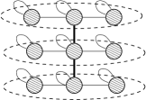
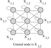
(a) Graph ${{K}}_{1}$	(b) Intermediate stage	(c) Graph ${{K}}_{2}={{K}}_{1}\otimes{{K}}_{1}$
(d) Adjacency matrix		(e) Adjacency matrix
of ${{K}}_{1}$		of ${{K}}_{2}={{K}}_{1}\otimes{{K}}_{1}$

Figure 1: Example of Kronecker multiplication: Top: a “3-chain” initiator graph and its Kronecker product with itself. Each of the $X_{i}$ nodes gets expanded into $3$ nodes, which are then linked using Observation 1. Bottom row: the corresponding adjacency matrices. See figure 2 for adjacency matrices of ${{K}}_{3}$ and ${{K}}_{4}$.

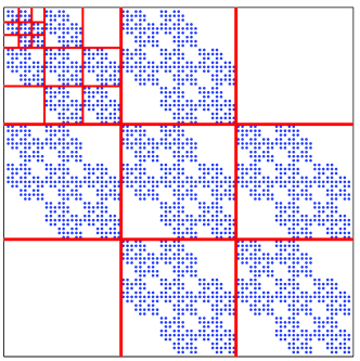
(a) ${{K}}_{3}$ adjacency matrix ($27\times 27$)		(b) ${{K}}_{4}$ adjacency matrix ($81\times 81$)

Figure 2: Adjacency matrices of ${{K}}_{3}$ and ${{K}}_{4}$, the $3^{rd}$ and $4^{th}$ Kronecker power of ${{K}}_{1}$ matrix as defined in Figure 1. Dots represent non-zero matrix entries, and white space represents zeros. Notice the recursive self-similar structure of the adjacency matrix.

Observation 1 (Edges in Kronecker-multiplied graphs)

$$\mbox{Edge~{}}(X_{ij},X_{kl})\in G\otimes H\mbox{~{}iff~{}}(X_{i},X_{k})\in G\mbox{~{}and~{}}(X_{j},X_{l})\in H$$

where $X_{ij}$ and $X_{kl}$ are nodes in $G\otimes H$, and $X_{i}$, $X_{j}$, $X_{k}$ and $X_{l}$ are the corresponding nodes in $G$ and $H$, as in Figure 1.

The last observation is crucial, and deserves elaboration. Basically, each node in $G\otimes H$ can be represented as an ordered pair $X_{ij}$, with $i$ a node of $G$ and $j$ a node of $H$, and with an edge joining $X_{ij}$ and $X_{kl}$ precisely when $(X_{i},X_{k})$ is an edge of $G$ and $(X_{j},X_{l})$ is an edge of $H$. This is a direct consequence of the hierarchical nature of the Kronecker product. Figure 1(a–c) further illustrates this by showing the recursive construction of $G\otimes H$, when $G=H$ is a 3-node chain. Consider node $X_{1,2}$ in Figure 1(c): It belongs to the $H$ graph that replaced node $X_{1}$ (see Figure 1(b)), and in fact is the $X_{2}$ node (i.e., the center) within this small $H$-graph.

We propose to produce a growing sequence of matrices by iterating the Kronecker product:

Definition 3 (Kronecker power)

The $k^{th}$ power of ${{K}}_{1}$ is defined as the matrix ${{K}}_{1}^{[k]}$ (abbreviated to ${{K}}_{k}$), such that:

$${{K}}_{1}^{[k]}={{K}}_{k}=\mbox{\raisebox{-7.5pt}{$\begin{array}[]{c}\underbrace{{{K}}_{1}\otimes{{K}}_{1}\otimes\ldots{{K}}_{1}}\\ k\mbox{~{}times}\end{array}$}}~{}=~{}{{K}}_{k-1}\otimes{{K}}_{1}$$ (4)

Definition 4 (Kronecker graph)

Kronecker graph of order $k$ is defined by the adjacency matrix ${{K}}_{1}^{[k]}$, where ${{K}}_{1}$ is the Kronecker initiator adjacency matrix.

The self-similar nature of the Kronecker graph product is clear: To produce ${{K}}_{k}$ from ${{K}}_{k-1}$, we “expand” (replace) each node of ${{K}}_{k-1}$ by converting it into a copy of ${{K}}_{1}$, and we join these copies together according to the adjacencies in ${{K}}_{k-1}$ (see Figure 1). This process is very natural: one can imagine it as positing that communities within the graph grow recursively, with nodes in the community recursively getting expanded into miniature copies of the community. Nodes in the sub-community then link among themselves and also to nodes from other communities.

Note that there are many different names to refer to Kronecker product of graphs. Other names for the Kronecker product are tensor product, categorical product, direct product, cardinal product, relational product, conjunction, weak direct product or just product, and even Cartesian product Imrich and Klavžar (2000).

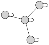
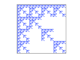
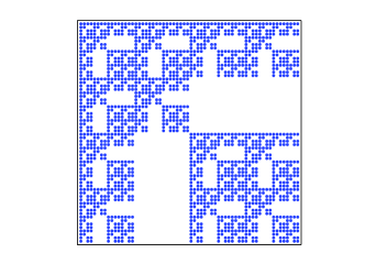
Initiator ${{K}}_{1}$	${{K}}_{1}$ adjacency matrix	${{K}}_{3}$ adjacency matrix

Figure 3: Two examples of Kronecker initiators on 4 nodes and the self-similar adjacency matrices they produce.

3.2 Analysis of Kronecker graphs

We shall now discuss the properties of Kronecker graphs, specifically, their degree distributions, diameters, eigenvalues, eigenvectors, and time-evolution. Our ability to prove analytical results about all of these properties is a major advantage of Kronecker graphs over other network models.

3.2.1 Degree distribution

The next few theorems prove that several distributions of interest are multinomial for our Kronecker graph model. This is important, because a careful choice of the initial graph ${{K}}_{1}$ makes the resulting multinomial distribution to behave like a power law or Discrete Gaussian Exponential (DGX) distribution Bi et al. (2001); Clauset et al. (2007).

Theorem 5 (Multinomial degree distribution)

Kronecker graphs have multinomial degree distributions, for both in- and out-degrees.

Proof  Let the initiator ${{K}}_{1}$ have the degree sequence $d_{1},d_{2},\ldots,d_{N_{1}}$. Kronecker multiplication of a node with degree $d$ expands it into $N_{1}$ nodes, with the corresponding degrees being $d\times d_{1},d\times d_{2},\ldots,d\times d_{N_{1}}$. After Kronecker powering, the degree of each node in graph ${{K}}_{k}$ is of the form $d_{i_{1}}\times d_{i_{2}}\times\ldots d_{i_{k}}$, with $i_{1},i_{2},\ldots,i_{k}\in(1\ldots N_{1})$, and there is one node for each ordered combination. This gives us the multinomial distribution on the degrees of ${{K}}_{k}$. So, graph ${{K}}_{k}$ will have multinomial degree distribution where the “events” (degrees) of the distribution will be combinations of degree products: $d_{1}^{i_{1}}d_{2}^{i_{2}}\dots d_{N_{1}}^{i_{N_{1}}}$ (where $\sum_{j=1}^{N_{1}}i_{j}=k$) and event (degree) probabilities will be proportional to ${k\choose i_{1}i_{2}\dots i_{N_{1}}}$. Note also that this is equivalent to noticing that the degrees of nodes in ${{K}}_{k}$ can be expressed as the $k^{th}$ Kronecker power of the vector $(d_{1},d_{2},\dots,d_{N_{1}})$.  

3.2.2 Spectral properties

Next we analyze the spectral properties of adjacency matrix of a Kronecker graph. We show that both the distribution of eigenvalues and the distribution of component values of eigenvectors of the graph adjacency matrix follow multinomial distributions.

Theorem 6 (Multinomial eigenvalue distribution)

The Kronecker graph ${{K}}_{k}$ has a multinomial distribution for its eigenvalues.

Proof  Let ${{K}}_{1}$ have the eigenvalues $\lambda_{1},\lambda_{2},\ldots,\lambda_{N_{1}}$. By properties of the Kronecker multiplication Loan (2000); Langville and Stewart (2004), the eigenvalues of ${{K}}_{k}$ are the $k^{th}$ Kronecker power of the vector of eigenvalues of the initiator matrix, $(\lambda_{1},\lambda_{2},\ldots,\lambda_{N_{1}})^{[k]}$. As in Theorem 5, the eigenvalue distribution is a multinomial.  

A similar argument using properties of Kronecker matrix multiplication shows the following.

Theorem 7 (Multinomial eigenvector distribution)

The components of each eigenvector of the Kronecker graph ${{K}}_{k}$ follow a multinomial distribution.

Proof  Let ${{K}}_{1}$ have the eigenvectors $\vec{v}_{1},\vec{v}_{2},\ldots,\vec{v}_{N_{1}}$. By properties of the Kronecker multiplication Loan (2000); Langville and Stewart (2004), the eigenvectors of ${{K}}_{k}$ are given by the $k^{th}$ Kronecker power of the vector: $(\vec{v}_{1},\vec{v}_{2},\ldots,\vec{v}_{{N}_{1}})$, which gives a multinomial distribution for the components of each eigenvector in ${{K}}_{k}$.  

We have just covered several of the static graph patterns. Notice that the proofs were a direct consequences of the Kronecker multiplication properties.

3.2.3 Connectivity of Kronecker graphs

We now present a series of results on the connectivity of Kronecker graphs. We show, maybe a bit surprisingly, that even if a Kronecker initiator graph is connected its Kronecker power can in fact be disconnected.

Lemma 8

If at least one of $G$ and $H$ is a disconnected graph, then $G\otimes H$ is also disconnected.

Proof  Without loss of generality we can assume that $G$ has two connected components, while $H$ is connected. Figure 4(a) illustrates the corresponding adjacency matrix for $G$. Using the notation from Observation 1 let graph let $G$ have nodes $X_{1},\ldots,X_{n}$, where nodes $\{X_{1},\ldots X_{r}\}$ and $\{X_{r+1},\ldots,X_{n}\}$ form the two connected components. Now, note that $(X_{ij},X_{kl})\notin G\otimes H$ for $i\in\{1,\ldots,r\}$, $k\in\{r+1,\ldots,n\}$, and all $j$, $l$. This follows directly from Observation 1 as $(X_{i},X_{k})$ are not edges in $G$. Thus, $G\otimes H$ must at least two connected components.  

Actually it turns out that both $G$ and $H$ can be connected while $G\otimes H$ is disconnected. The following theorem analyzes this case.

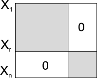
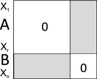
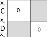
(a) Adjacency matrix		(b) Adjacency matrix		(c) Adjacency matrix
when $G$ is disconnected		when $G$ is bipartite		when $H$ is bipartite

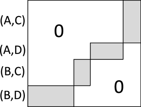
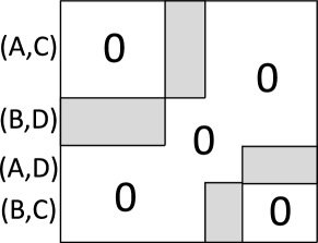
(d) Kronecker product of		(e) Rearranged adjacency
two bipartite graphs $G$ and $H$		matrix from panel (d)

Figure 4: Graph adjacency matrices. Dark parts represent connected (filled with ones) and white parts represent empty (filled with zeros) parts of the adjacency matrix. (a) When $G$ is disconnected, Kronecker multiplication with any matrix $H$ will result in $G\otimes H$ being disconnected. (b) Adjacency matrix of a connected bipartite graph $G$ with node partitions $A$ and $B$. (c) Adjacency matrix of a connected bipartite graph $G$ with node partitions $C$ and $D$. (e) Kronecker product of two bipartite graphs $G$ and $H$. (d) After rearranging the adjacency matrix $G\otimes H$ we clearly see the resulting graph is disconnected.

Theorem 9

If both $G$ and $H$ are connected but bipartite, then $G\otimes H$ is disconnected, and each of the two connected components is again bipartite.

Proof  Again without loss of generality let $G$ be bipartite with two partitions $A=\{X_{1},\ldots X_{r}\}$ and $B=\{X_{r+1},\ldots,X_{n}\}$, where edges exists only between the partitions, and no edges exist inside the partition: $(X_{i},X_{k})\notin G$ for $i,k\in A$ or $i,k\in B$. Similarly, let $H$ also be bipartite with two partitions $C=\{X_{1},\ldots X_{s}\}$ and $D=\{X_{s+1},\ldots,X_{m}\}$. Figures 4(b) and (c) illustrate the structure of the corresponding adjacency matrices.

Now, there will be two connected components in $G\otimes H$: $1^{st}$ component will be composed of nodes $\{X_{ij}\}\in G\otimes H$, where $(i\in A,j\in D)$ or $(i\in B,j\in C)$. And similarly, $2^{nd}$ component will be composed of nodes $\{X_{ij}\}$, where $(i\in A,j\in C)$ or $(i\in B,j\in D)$. Basically, there exist edges between node sets $(A,D)$ and $(B,C)$, and similarly between $(A,C)$ and $(B,D)$ but not across the sets. To see this we have to analyze the cases using Observation 1. For example, in $G\otimes H$ there exist edges between nodes $(A,C)$ and $(B,D)$ as there exist edges $(i,k)\in G$ for $i\in A,k\in B$, and $(j,l)\in H$ for $j\in C$ and $l\in D$. Similar is true for nodes $(A,C)$ and $(B,D)$. However, there are no edges cross the two sets, e.g., nodes from $(A,D)$ do not link to $(A,C)$, as there are no edges between nodes in $A$ (since $G$ is bipartite). See Figures 4(d) and 4(e) for a visual proof.  

Note that bipartite graphs are triangle free and have no self-loops. Stars, chains, trees and cycles of even length are all examples of bipartite graphs. In order to ensure that ${{K}}_{k}$ is connected, for the remained of the paper we focus on initiator graphs ${{K}}_{1}$ with self loops on all of the vertices.

3.2.4 Temporal properties of Kronecker graphs

We continue with the analysis of temporal patterns of evolution of Kronecker graphs: the densification power law, and shrinking/stabilizing diameter Leskovec et al. (2005b, 2007a).

Theorem 10 (Densification power law)

Kronecker graphs follow the densification power law (DPL) with densification exponent $a=\log({E}_{1})/\log({N}_{1})$.

Proof  Since the $k^{\rm th}$ Kronecker power ${{K}}_{k}$ has ${N}_{k}={N}_{1}^{k}$ nodes and ${E}_{k}={E}_{1}^{k}$ edges, it satisfies ${E}_{k}={N}_{k}^{a}$, where $a=\log({E}_{1})/\log({N}_{1})$. The crucial point is that this exponent $a$ is independent of $k$, and hence the sequence of Kronecker powers follows an exact version of the densification power law.  

We now show how the Kronecker product also preserves the property of constant diameter, a crucial ingredient for matching the diameter properties of many real-world network datasets. In order to establish this, we will assume that the initiator graph ${{K}}_{1}$ has a self-loop on every node. Otherwise, its Kronecker powers may be disconnected.

Lemma 11

If $G$ and $H$ each have diameter at most $D$ and each has a self-loop on every node, then the Kronecker graph $G\otimes H$ also has diameter at most $D$.

Proof  Each node in $G\otimes H$ can be represented as an ordered pair $(v,w)$, with $v$ a node of $G$ and $w$ a node of $H$, and with an edge joining $(v,w)$ and $(x,y)$ precisely when $(v,x)$ is an edge of $G$ and $(w,y)$ is an edge of $H$. (Note this exactly the Observation 1.) Now, for an arbitrary pair of nodes $(v,w)$ and $(v^{\prime},w^{\prime})$, we must show that there is a path of length at most $D$ connecting them. Since $G$ has diameter at most $D$, there is a path $v=v_{1},v_{2},\ldots,v_{r}=v^{\prime}$, where $r\leq D$. If $r<D$, we can convert this into a path $v=v_{1},v_{2},\ldots,v_{D}=v^{\prime}$ of length exactly $D$, by simply repeating $v^{\prime}$ at the end for $D-r$ times. By an analogous argument, we have a path $w=w_{1},w_{2},\ldots,w_{D}=w^{\prime}$. Now by the definition of the Kronecker product, there is an edge joining $(v_{i},w_{i})$ and $(v_{i+1},w_{i+1})$ for all $1\leq i\leq D-1$, and so $(v,w)=(v_{1},w_{1}),(v_{2},w_{2}),\ldots,(v_{D},w_{D})=(v^{\prime},w^{\prime})$ is a path of length $D$ connecting $(v,w)$ to $(v^{\prime},w^{\prime})$, as required.  

Theorem 12

If ${{K}}_{1}$ has diameter $D$ and a self-loop on every node, then for every $k$, the graph ${{K}}_{k}$ also has diameter $D$.

Proof  This follows directly from the previous lemma, combined with induction on $k$.  

As defined in section 2 we also consider the effective diameter $D^{*}$. We defined the $q$-effective diameter as the minimum $D^{*}$ such that, for a $q$ fraction of the reachable node pairs, the path length is at most $D^{*}$. The $q$-effective diameter is a more robust quantity than the diameter, the latter being prone to the effects of degenerate structures in the graph (e.g., very long chains). However, the $q$-effective diameter and diameter tend to exhibit qualitatively similar behavior. For reporting results in subsequent sections, we will generally consider the $q$-effective diameter with $q=0.9$, and refer to this simply as the effective diameter.

Theorem 13 (Effective Diameter)

If ${{K}}_{1}$ has diameter $D$ and a self-loop on every node, then for every $q$, the $q$-effective diameter of ${{K}}_{k}$ converges to $D$ (from below) as $k$ increases.

Proof  To prove this, it is sufficient to show that for two randomly selected nodes of ${{K}}_{k}$, the probability that their distance is $D$ converges to $1$ as $k$ goes to infinity.

We establish this as follows. Each node in ${{K}}_{k}$ can be represented as an ordered sequence of $k$ nodes from ${{K}}_{1}$, and we can view the random selection of a node in ${{K}}_{k}$ as a sequence of $k$ independent random node selections from ${{K}}_{1}$. Suppose that $v=(v_{1},\ldots,v_{k})$ and $w=(w_{1},\ldots,w_{k})$ are two such randomly selected nodes from ${{K}}_{k}$. Now, if $x$ and $y$ are two nodes in ${{K}}_{1}$ at distance $D$ (such a pair $(x,y)$ exists since ${{K}}_{1}$ has diameter $D$), then with probability $1-(1-\frac{1}{{N}_{1}^{2}})^{k}$, there is some index $j$ for which $\{v_{j},w_{j}\}=\{x,y\}$. If there is such an index, then the distance between $v$ and $w$ is $D$. As the expression $1-(1-\frac{1}{{N}_{1}^{2}})^{k}$ converges to $1$ as $k$ increases, it follows that the $q$-effective diameter is converging to $D$.  

3.3 Stochastic Kronecker graphs

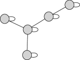
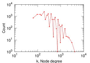
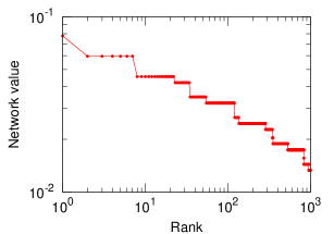
(a) Kronecker	(b) Degree distribution of ${{K}}_{6}$	(c) Network value of ${{K}}_{6}$
initiator ${{K}}_{1}$	($6^{th}$ Kronecker power of ${{K}}_{1}$)	($6^{th}$ Kronecker power of ${{K}}_{1}$)

Figure 5: The “staircase” effect. Kronecker initiator and the degree distribution and network value plot for the $6^{th}$ Kronecker power of the initiator. Notice the non-smoothness of the curves.

While the Kronecker power construction discussed so far yields graphs with a range of desired properties, its discrete nature produces “staircase effects” in the degrees and spectral quantities, simply because individual values have large multiplicities. For example, degree distribution and distribution of eigenvalues of graph adjacency matrix and the distribution of the principal eigenvector components (i.e., the “network” value) are all impacted by this. These quantities are multinomially distributed which leads to individual values with large multiplicities. Figure 5 illustrates the staircase effect.

Here we propose a stochastic version of Kronecker graphs that eliminates this effect. There are many possible ways how one could introduce stochasticity into Kronecker graph model. Before introducing the proposed model, we introduce two simple ways of introducing randomness to Kronecker graphs and describe why they do not work.

Probably the simplest (but wrong) idea is to generate a large deterministic Kronecker graph ${{K}}_{k}$, and then uniformly at random flip some edges, i.e., uniformly at random select entries of the graph adjacency matrix and flip them ($1\rightarrow 0,0\rightarrow 1$). However, this will not work, as it will essentially superimpose an Erdős-Rényi random graph, which would, for example, corrupt the degree distribution – real networks usually have heavy tailed degree distributions, while random graphs have Binomial degree distributions. A second idea could be to allow a weighted initiator matrix, i.e., values of entries of ${{K}}_{1}$ are not restricted to values $\{0,1\}$ but rather can be any non-negative real number. Using such ${{K}}_{1}$ one would generate ${{K}}_{k}$ and then threshold the ${{K}}_{k}$ matrix to obtain a binary adjacency matrix $K$, i.e., for a chosen value of $\epsilon$ set $K[i,j]=1$ if ${{K}}_{k}[i,j]>\epsilon$ else $K[i,j]=0$. This also would not work as the mechanism would selectively remove edges and thus the low degree nodes which would have low weight edges would get isolated first.

Now we define Stochastic Kronecker graph model which overcomes the above issues. A more natural way to introduce stochasticity to Kronecker graphs is to relax the assumption that entries of the initiator matrix take only binary values. Instead we allow entries of the initiator to take values on the interval $[0,1]$. This means now each entry of the initiator matrix encodes the probability of that particular edge appearing. We then Kronecker-power such initiator matrix to obtain a large stochastic adjacency matrix, where again each entry of the large matrix gives the probability of that particular edge appearing in a big graph. Such a stochastic adjacency matrix defines a probability distribution over all graphs. To obtain a graph we simply sample an instance from this distribution by sampling individual edges, where each edge appears independently with probability given by the entry of the large stochastic adjacency matrix. More formally, we define:

Definition 14 (Stochastic Kronecker graph)

Let ${\cal P}_{1}$ be a ${N}_{1}\times{N}_{1}$ probability matrix: the value ${\theta_{{ij}}}\in{\cal P}_{1}$ denotes the probability that edge $(i,j)$ is present, ${\theta_{{ij}}}\in[0,1]$.

Then $k^{th}$ Kronecker power ${\cal P}_{1}^{[k]}={\cal P}_{k}$, where each entry $p_{uv}\in{\cal P}_{k}$ encodes the probability of an edge $(u,v)$.

To obtain a graph, an instance (or realization), $K=R({\cal P}_{k})$ we include edge $(u,v)$ in $K$ with probability $p_{uv}$, $p_{uv}\in{\cal P}_{k}$.

First, note that sum of the entries of ${\cal P}_{1}$, $\sum_{ij}{\theta_{{ij}}}$, can be greater than 1. Second, notice that in principle it takes $O({N}_{1}^{2k})$ time to generate an instance $K$ of a Stochastic Kronecker graph from the probability matrix ${\cal P}_{k}$. This means the time to get a realization $K$ is quadratic in the size of ${\cal P}_{k}$ as one has to flip a coin for each possible edge in the graph. Later we show how to generate Stochastic Kronecker graphs much faster, in the time linear in the expected number of edges in ${\cal P}_{k}$.

3.3.1 Probability of an edge

For the size of graphs we aim to model and generate here taking ${\cal P}_{1}$ (or ${{K}}_{1}$) and then explicitly performing the Kronecker product of the initiator matrix is infeasible. The reason for this is that ${\cal P}_{1}$ is usually dense, so ${\cal P}_{k}$ is also dense and one can not explicitly store it in memory to directly iterate the Kronecker product. However, due to the structure of Kronecker multiplication one can easily compute the probability of an edge in ${\cal P}_{k}$.

The probability ${p_{{uv}}}$ of an edge $(u,v)$ occurring in $k$-th Kronecker power ${\cal P}={\cal P}_{k}$ can be calculated in $O(k)$ time as follows:

$${p_{{uv}}}=\prod_{i=0}^{k-1}{\cal P}_{1}\biggl{[}\Bigl{\lfloor}\frac{u-1}{{N}_{1}^{i}}\Bigr{\rfloor}({\textrm{mod}}{N}_{1})+1,\Bigl{\lfloor}\frac{v-1}{{N}_{1}^{i}}\Bigr{\rfloor}({\textrm{mod}}{N}_{1})+1\biggr{]}$$ (5)

The equation imitates recursive descent into the matrix ${\cal P}$, where at every level $i$ the appropriate entry of ${\cal P}_{1}$ is chosen. Since ${\cal P}$ has ${N}_{1}^{k}$ rows and columns it takes $O(k\log{N}_{1})$ to evaluate the equation. Refer to Figure 6 for the illustration of the recursive structure of ${\cal P}$.

3.4 Additional properties of Kronecker graphs

Stochastic Kronecker graphs with initiator matrix of size ${N}_{1}=2$ were studied by Mahdian and Xu Mahdian and Xu (2007). The authors showed a phase transition for the emergence of the giant component and another phase transition for connectivity, and proved that such graphs have constant diameters beyond the connectivity threshold, but are not searchable using a decentralized algorithm Kleinberg (1999).

General overview of Kronecker product is given in Imrich and Klavžar (2000) and properties of Kronecker graphs related to graph minors, planarity, cut vertex and cut edge have been explored in Bottreau and Metivier (1998). Moreover, recently Tsourakakis (2008) gave a closed form expression for the number of triangles in a Kronecker graph that depends on the eigenvalues of the initiator graph ${{K}}_{1}$.

3.5 Two interpretations of Kronecker graphs

Next, we present two natural interpretations of the generative process behind the Kronecker graphs that go beyond the purely mathematical construction of Kronecker graphs as introduced so far.

We already mentioned the first interpretation when we first defined Kronecker graphs. One intuition is that networks are hierarchically organized into communities (clusters). Communities then grow recursively, creating miniature copies of themselves. Figure 1 depicts the process of the recursive community expansion. In fact, several researchers have argued that real networks are hierarchically organized Ravasz et al. (2002); Ravasz and Barabási (2003) and algorithms to extract the network hierarchical structure have also been developed Sales-Pardo et al. (2007); Clauset et al. (2008). Moreover, especially web graphs Dill et al. (2002); Dorogovtsev et al. (2002); Crovella and Bestavros (1997) and biological networks Ravasz and Barabási (2003) were found to be self-similar and “fractal”.

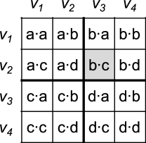
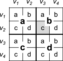
(a) $2\times 2$ Stochastic		(b) Probability matrix		(c) Alternative view
Kronecker initiator ${\cal P}_{1}$		${\cal P}_{2}={\cal P}_{1}\otimes{\cal P}_{1}$		of ${\cal P}_{2}={\cal P}_{1}\otimes{\cal P}_{1}$

Figure 6: Stochastic Kronecker initiator ${\cal P}_{1}$ and the corresponding $2^{nd}$ Kronecker power ${\cal P}_{2}$. Notice the recursive nature of the Kronecker product, with edge probabilities in ${\cal P}_{2}$ simply being products of entries of ${\cal P}_{1}$.

The second intuition comes from viewing every node of ${\cal P}_{k}$ as being described with an ordered sequence of $k$ nodes from ${\cal P}_{1}$. (This is similar to the Observation 1 and the proof of Theorem 13.)

Let’s label nodes of the initiator matrix ${\cal P}_{1}$, $u_{1},\ldots,u_{{N}_{1}}$, and nodes of ${\cal P}_{k}$ as $v_{1},\ldots,v_{{N}_{1}^{k}}$. Then every node $v_{i}$ of ${\cal P}_{k}$ is described with a sequence $(v_{i}(1),\ldots,v_{i}(k))$ of node labels of ${\cal P}_{1}$, where $v_{i}(l)\in\{u_{1},\ldots,u_{k}\}$. Similarly, consider also a second node $v_{j}$ with the label sequence $(v_{j}(1),\ldots,v_{j}(k))$. Then the probability $p_{e}$ of an edge $(v_{i},v_{j})$ in ${\cal P}_{k}$ is exactly:

$$p_{e}(v_{i},v_{j})={\cal P}_{k}[v_{i},v_{j}]=\prod_{l=1}^{k}{\cal P}_{1}[v_{i}(l),v_{j}(l)]$$

(Note this is exactly the Equation 5.)

Now one can look at the description sequence of node $v_{i}$ as a $k$ dimensional vector of attribute values $(v_{i}(1),\ldots,v_{i}(k))$. Then $p_{e}(v_{i},v_{j})$ is exactly the coordinate-wise product of appropriate entries of ${\cal P}_{1}$, where the node description sequence selects which entries of ${\cal P}_{1}$ to multiply. Thus, the ${\cal P}_{1}$ matrix can be thought of as the attribute similarity matrix, i.e., it encodes the probability of linking given that two nodes agree/disagree on the attribute value. Then the probability of an edge is simply a product of individual attribute similarities over the $k$ ${N}_{1}$-valued attributes that describe each of the two nodes.

This gives us a very natural interpretation of Stochastic Kronecker graphs: Each node is described by a sequence of categorical attribute values or features. And then the probability of two nodes linking depends on the product of individual attribute similarities. This way Kronecker graphs can effectively model homophily (nodes with similar attribute values are more likely to link) by ${\cal P}_{1}$ having high value entries on the diagonal. Or heterophily (nodes that differ are more likely to link) by ${\cal P}_{1}$ having high entries off the diagonal.

Figure 6 shows an example. Let’s label nodes of ${\cal P}_{1}$ $u_{1},u_{2}$ as in Figure 6(a). Then every node of ${\cal P}_{k}$ is described with an ordered sequence of $k$ binary attributes. For example, Figure 6(b) shows an instance for $k=2$ where node $v_{2}$ of ${\cal P}_{2}$ is described by $(u_{1},u_{2})$, and similarly $v_{3}$ by $(u_{2},u_{1})$. Then as shown in Figure 6(b), the probability of edge $p_{e}(v_{2},v_{3})=b\cdot c$, which is exactly ${\cal P}_{1}[u_{2},u_{1}]\cdot{\cal P}_{1}[u_{1},u_{2}]=b\cdot c$ — the product of entries of ${\cal P}_{1}$, where the corresponding elements of the description of nodes $v_{2}$ and $v_{3}$ act as selectors of which entries of ${\cal P}_{1}$ to multiply.

Figure 6(c) further illustrates the recursive nature of Kronecker graphs. One can see Kronecker product as recursive descent into the big adjacency matrix where at each stage one of the entries or blocks is chosen. For example, to get to entry $(v_{2},v_{3})$ one first needs to dive into quadrant $b$ following by the quadrant $c$. This intuition will help us in section 3.6 to devise a fast algorithm for generating Kronecker graphs.

However, there are also two notes to make here. First, using a single initiator ${\cal P}_{1}$ we are implicitly assuming that there is one single and universal attribute similarity matrix that holds across all $k$ ${N}_{1}$-ary attributes. One can easily relax this assumption by taking a different initiator matrix for each attribute (initiator matrices can even be of different sizes as attributes are of different arity), and then Kronecker multiplying them to obtain a large network. Here each initiator matrix plays the role of attribute similarity matrix for that particular attribute.

For simplicity and convenience we will work with a single initiator matrix but all our methods can be trivially extended to handle multiple initiator matrices. Moreover, as we will see later in section 6 even a single $2\times 2$ initiator matrix seems to be enough to capture large scale statistical properties of real-world networks.

The second assumption is harder to relax. When describing every node $v_{i}$ with a sequence of attribute values we are implicitly assuming that the values of all attributes are uniformly distributed (have same proportions), and that every node has a unique combination of attribute values. So, all possible combinations of attribute values are taken. For example, node $v_{1}$ in a large matrix ${\cal P}_{k}$ has attribute sequence $(u_{1},u_{1},\ldots,u_{1})$, and $v_{{N}_{1}}$ has $(u_{1},u_{1},\ldots,u_{1},u_{{N}_{1}})$, while the “last” node $v_{{N}_{1}^{k}}$ is has attribute values $(u_{{N}_{1}},u_{{N}_{1}},\ldots,u_{{N}_{1}})$. One can think of this as counting in ${N}_{1}$-ary number system, where node attribute descriptions range from $0$ (i.e., “leftmost” node with attribute description $(u_{1},u_{1},\ldots,u_{1})$) to ${N}_{1}^{k}$ (i.e., “rightmost” node attribute description $(u_{{N}_{1}},u_{{N}_{1}},\ldots,u_{{N}_{1}})$).

A simple way to relax the above assumption is to take a larger initiator matrix with a smaller number of parameters than the number of entries. This means that multiple entries of ${\cal P}_{1}$ will share the same value (parameter). For example, if attribute $u_{1}$ takes one value 66% of the times, and the other value 33% of the times, then one can model this by taking a $3\times 3$ initiator matrix with only four parameters. Adopting the naming convention of Figure 6 this means that parameter $a$ now occupies a $2\times 2$ block, which then also makes $b$ and $c$ occupy $2\times 1$ and $1\times 2$ blocks, and $d$ a single cell. This way one gets a four parameter model with uneven feature value distribution.

We note that the view of Kronecker graphs where every node is described with a set of features and the initiator matrix encodes the probability of linking given the attribute values of two nodes somewhat resembles the Random dot product graph model Young and Scheinerman (2007); Nickel (2008). The important difference here is that we multiply individual linking probabilities, while in Random dot product graphs one takes the sum of individual probabilities which seems somewhat less natural.

3.6 Fast generation of Stochastic Kronecker graphs

The intuition for fast generation of Stochastic Kronecker graphs comes from the recursive nature of the Kronecker product and is closely related to the R-MAT graph generator Chakrabarti et al. (2004). Generating a Stochastic Kronecker graph $K$ on $N$ nodes naively takes $O(N^{2})$ time. Here we present a linear time $O(E)$ algorithm, where $E$ is the (expected) number of edges in $K$.

Figure 6(c) shows the recursive nature of the Kronecker product. To “arrive” to a particular edge $(v_{i},v_{j})$ of ${\cal P}_{k}$ one has to make a sequence of $k$ (in our case $k=2$) decisions among the entries of ${\cal P}_{1}$, multiply the chosen entries of ${\cal P}_{1}$, and then placing the edge $(v_{i},v_{j})$ with the obtained probability.

Instead of flipping $O(N^{2})=O({N}_{1}^{2k})$ biased coins to determine the edges, we can place $E$ edges by directly simulating the recursion of the Kronecker product. Basically we recursively choose sub-regions of matrix $K$ with probability proportional to ${\theta_{{ij}}}$, ${\theta_{{ij}}}\in{\cal P}_{1}$ until in $k$ steps we descend to a single cell of the big adjacency matrix $K$ and place an edge. For example, for $(v_{2},v_{3})$ in Figure 6(c) we first have to choose $b$ following by $c$.

The probability of each individual edge of ${\cal P}_{k}$ follows a Bernoulli distribution, as the edge occurrences are independent. By the Central Limit Theorem Petrov (1995) the number of edges in ${\cal P}_{k}$ tends to a normal distribution with mean $(\sum_{i,j=1}^{N_{1}}{\theta_{{ij}}})^{k}={E}_{1}^{k}$, where ${\theta_{{ij}}}\in{\cal P}_{1}$. So, given a stochastic initiator matrix ${\cal P}_{1}$ we first sample the expected number of edges $E$ in ${\cal P}_{k}$. Then we place $E$ edges in a graph ${K}$, by applying the recursive descent for $k$ steps where at each step we choose entry $(i,j)$ with probability ${\theta_{{ij}}}/{E}_{1}$ where ${E}_{1}=\sum_{ij}{\theta_{{ij}}}$. Since we add $E={E}_{1}^{k}$ edges, the probability that edge $(v_{i},v_{j})$ appears in ${K}$ is exactly ${\cal P}_{k}[v_{i},v_{j}]$. This basically means that in Stochastic Kronecker graphs the initiator matrix encodes both the total number of edges in a graph and their structure. $\sum{\theta_{{ij}}}$ encodes the number of edges in the graph, while the proportions (ratios) of values ${\theta_{{ij}}}$ define how many edges each part of graph adjacency matrix will contain.

In practice it can happen that more than one edge lands in the same $(v_{i},v_{j})$ entry of big adjacency matrix $K$. If an edge lands in a already occupied cell we insert it again. Even though values of ${\cal P}_{1}$ are usually skewed, adjacency matrices of real networks are so sparse that this is not really a problem in practice. Empirically we note that around 1% of edges collide.

3.7 Observations and connections

Next, we describe several observations about the properties of Kronecker graphs and make connections to other network models.

• Bipartite graphs: Kronecker graphs can naturally model bipartite graphs. Instead of starting with a square ${N}_{1}\times{N}_{1}$ initiator matrix, one can choose arbitrary ${N}_{1}\times M_{1}$ initiator matrix, where rows define “left”, and columns the “right” side of the bipartite graph. Kronecker multiplication will then generate bipartite graphs with partition sizes ${N}_{1}^{k}$ and $M_{1}^{k}$.

• Graph distributions: ${\cal P}_{k}$ defines a distribution over all graphs, as it encodes the probability of all possible ${N}_{1}^{2k}$ edges appearing in a graph by using an exponentially smaller number of parameters (just ${N}_{1}^{2}$). As we will later see, even a very small number of parameters, e.g., 4 ($2\times 2$ initiator matrix) or 9 ($3\times 3$ initiator), is enough to accurately model the structure of large networks.

• Extension of Erdős-Rényi random graph model: Stochastic Kronecker graphs represent an extension of Erdős-Rényi Erdős and Rényi (1960) random graphs. If one takes ${\cal P}_{1}=[{\theta_{{ij}}}]$, where every ${\theta_{{ij}}}=p$ then we obtain exactly the Erdős-Rényi model of random graphs $G_{n,p}$, where every edge appears independently with probability $p$.

• Relation to the R-MAT model: The recursive nature of Stochastic Kronecker graphs makes them related to the R-MAT generator Chakrabarti et al. (2004). The difference between the two models is that in R-MAT one needs to separately specify the number of edges, while in Stochastic Kronecker graphs initiator matrix ${\cal P}_{1}$ also encodes the number of edges in the graph. Section 3.6 built on this similarity to devise a fast algorithm for generating Stochastic Kronecker graphs.

• Densification: Similarly as with deterministic Kronecker graphs the number of nodes in a Stochastic Kronecker graph grows as ${N}_{1}^{k}$, and the expected number of edges grows as $(\sum_{ij}{\theta_{{ij}}})^{k}$. This means one would want to choose values ${\theta_{{ij}}}$ of the initiator matrix ${\cal P}_{1}$ so that $\sum_{ij}{\theta_{{ij}}}>{N}_{1}$ in order for the resulting network to densify.

4 Simulations of Kronecker graphs

Next we perform a set of simulation experiments to demonstrate the ability of Kronecker graphs to match the patterns of real-world networks. We will tackle the problem of estimating the Kronecker graph model from real data, i.e., finding the most likely initiator ${\cal P}_{1}$, in the next section. Instead here we present simulation experiments using Kronecker graphs to explore the parameter space, and to compare properties of Kronecker graphs to those found in large real networks.

4.1 Comparison to real graphs

We observe two kinds of graph patterns — “static” and “temporal.” As mentioned earlier, common static patterns include degree distribution, scree plot (eigenvalues of graph adjacency matrix vs. rank) and distribution of components of the principal eigenvector of graph adjacency matrix. Temporal patterns include the diameter over time, and the densification power law. For the diameter computation, we use the effective diameter as defined in Section 2.

For the purpose of this section consider the following setting. Given a real graph ${G}$ we want to find Kronecker initiator that produces qualitatively similar graph. In principle one could try choosing each of the ${N}_{1}^{2}$ parameters for the matrix ${\cal P}_{1}$ separately. However, we reduce the number of parameters from ${N}_{1}^{2}$ to just two: $\alpha$ and $\beta$. Let ${{K}}_{1}$ be the initiator matrix (binary, deterministic). Then we create the corresponding stochastic initiator matrix ${\cal P}_{1}$ by replacing each “1” and “0” of ${{K}}_{1}$ with $\alpha$ and $\beta$ respectively ($\beta\leq\alpha$). The resulting probability matrices maintain — with some random noise — the self-similar structure of the Kronecker graphs in the previous section (which, for clarity, we call deterministic Kronecker graphs). We defer the discussion of how to automatically estimate ${\cal P}_{1}$ from data $G$ to the next section.

The datasets we use here are:

• Cit-hep-th: This is a citation graph for High-Energy Physics Theory research papers from pre-print archive ArXiv, with a total of $N=$29,555 papers and $E=$352,807 citations Gehrke et al. (2003). We follow its evolution from January 1993 to April 2003, with one data-point per month.

• As-RouteViews: We also analyze a static dataset consisting of a single snapshot of connectivity among Internet Autonomous Systems RouteViews (1997) from January 2000, with $N=$6,474 and $E=$26,467.

Results are shown in Figure 7 for the Cit-hep-th graph which evolves over time. We show the plots of two static and two temporal patterns. We see that the deterministic Kronecker model already to some degree captures the qualitative structure of the degree and eigenvalue distributions, as well as the temporal patterns represented by the densification power law and the stabilizing diameter. However, the deterministic nature of this model results in “staircase” behavior, as shown in scree plot for the deterministic Kronecker graph of Figure 7 (column (b), second row). We see that the Stochastic Kronecker graphs smooth out these distributions, further matching the qualitative structure of the real data, and they also match the shrinking-before-stabilization trend of the diameters of real graphs.

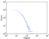
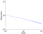
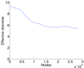
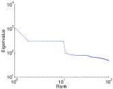
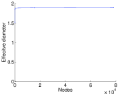
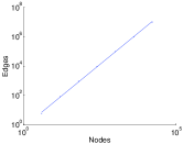
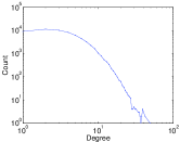
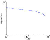
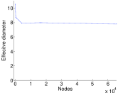
	(a) Degree	(b) Scree plot	(c) Diameter	(d) DPL
	distribution		over time

Figure 7: Citation network (Cit-hep-th): Patterns from the real graph (top row), the deterministic Kronecker graph with ${{K}}_{1}$ being a star graph on 4 nodes (center + 3 satellites) (middle row), and the Stochastic Kronecker graph ($\alpha=0.41,~{}\beta=0.11$ – bottom row). Static patterns: (a) is the PDF of degrees in the graph (log-log scale), and (b) the distribution of eigenvalues (log-log scale). Temporal patterns: (c) gives the effective diameter over time (linear-linear scale), and (d) is the number of edges versus number of nodes over time (log-log scale). Notice that the Stochastic Kronecker graphs  qualitatively matches all the patterns very well.

Similarly, Figure 8 shows plots for the static patterns in the Autonomous systems (As-RouteViews) graph. Recall that we analyze a single, static network snapshot in this case. In addition to the degree distribution and scree plot, we also show two typical plots Chakrabarti et al. (2004): the distribution of network values (principal eigenvector components, sorted, versus rank) and the hop-plot (the number of reachable pairs $g(h)$ within $h$ hops or less, as a function of the number of hops $h$). Notice that, again, the Stochastic Kronecker graph matches well the properties of the real graph.

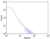
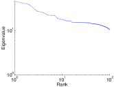
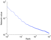
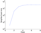
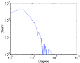
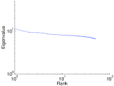
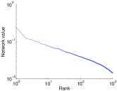
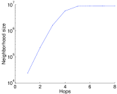
	(a) Degree	(b) Scree plot	(c) “Network value”	(d) “Hop-plot”
	distribution		distribution

Figure 8: Autonomous systems (As-RouteViews): Real (top) versus Kronecker (bottom). Columns (a) and (b) show the degree distribution and the scree plot, as before. Columns (c) and (d) show two more static patterns (see text). Notice that, again, the Stochastic Kronecker graph matches well the properties of the real graph.

4.2 Parameter space of Kronecker graphs

Last we present simulation experiments that investigate the parameter space of Stochastic Kronecker graphs.

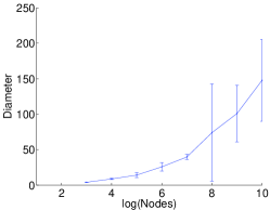
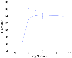
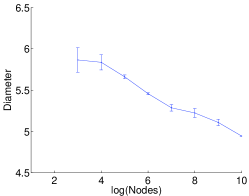
(a) Increasing diameter	(b) Constant diameter	(c) Decreasing diameter
$\alpha=0.38,\beta=0$	$\alpha=0.43,\beta=0$	$\alpha=0.54,\beta=0$

Figure 9: Effective diameter over time for a 4-node chain initiator graph. After each consecutive Kronecker power we measure the effective diameter. We use different settings of $\alpha$ parameter. $\alpha=0.38,0.43,0.54$ and $\beta=0$, respectively.

First, in Figure 9 we show the ability of Kronecker Graphs to generate networks with increasing, constant and decreasing/stabilizing effective diameter. We start with a 4-node chain initiator graph (shown in top row of Figure 3), setting each “1” of ${{K}}_{1}$ to $\alpha$ and each “0” to $\beta=0$ to obtain ${\cal P}_{1}$ that we then use to generate a growing sequence of graphs. We plot the effective diameter of each $R({\cal P}_{k})$ as we generate a sequence of growing graphs $R({\cal P}_{2}),R({\cal P}_{3}),\ldots,R({\cal P}_{10})$. $R({\cal P}_{10})$ has exactly 1,048,576 nodes. Notice Stochastic Kronecker graphs is a very flexible model. When the generated graph is very sparse (low value of $\alpha$) we obtain graphs with slowly increasing effective diameter (Figure 9(a)). For intermediate values of $\alpha$ we get graphs with constant diameter (Figure 9(b)) and that in our case also slowly densify with densification exponent $a=1.05$. Last, we see an example of a graph with shrinking/stabilizing effective diameter. Here we set the $\alpha=0.54$ which results in a densification exponent of $a=1.2$. Note that these observations are not contradicting Theorem 11. Actually, these simulations here agree well with the analysis of Mahdian and Xu (2007).

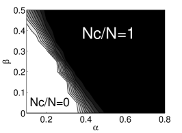
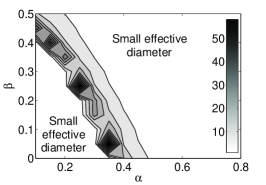
(a) Largest component size	(b) Largest component size	(c) Effective diameter

Figure 10: Fraction of nodes in the largest weakly connected component ($N_{c}/N$) and the effective diameter for 4-star initiator graph. (a) We fix $\beta=0.15$ and vary $\alpha$. (b) We vary both $\alpha$ and $\beta$. (c) Effective diameter of the network, if network is disconnected or very dense path lengths are short, the diameter is large when the network is barely connected.

Next, we examine the parameter space of a Stochastic Kronecker graphs where we choose a star on 4 nodes as a initiator graph and parameterized with $\alpha$ and $\beta$ as before. The initiator graph and the structure of the corresponding (deterministic) Kronecker graph adjacency matrix is shown in top row of Figure 3.

Figure 10(a) shows the sharp transition in the fraction of the number of nodes that belong to the largest weakly connected component as we fix $\beta=0.15$ and slowly increase $\alpha$. Such phase transitions on the size of the largest connected component also occur in Erdős-Rényi random graphs. Figure 10(b) further explores this by plotting the fraction of nodes in the largest connected component ($N_{c}/N$) over the full parameter space. Notice a sharp transition between disconnected (white area) and connected graphs (dark).

Last, Figure 10(c) shows the effective diameter over the parameter space $(\alpha,\beta)$ for the 4-node star initiator graph. Notice that when parameter values are small, the effective diameter is small, since the graph is disconnected and not many pairs of nodes can be reached. The shape of the transition between low-high diameter closely follows the shape of the emergence of the connected component. Similarly, when parameter values are large, the graph is very dense, and the diameter is small. There is a narrow band in parameter space where we get graphs with interesting diameters.

5 Kronecker graph model estimation

In previous sections we investigated various properties of networks generated by the (Stochastic) Kronecker graphs model. Many of these properties were also observed in real networks. Moreover, we also gave closed form expressions (parametric forms) for values of these statistical network properties, which allow us to calculate a property (e.g., diameter, eigenvalue spectrum) of a network directly from just the initiator matrix. So in principle, one could invert these equations and directly get from a property (e.g., shape of degree distribution) to the values of initiator matrix.

However, in previous sections we did not say anything about how various network properties of a Kronecker graph correlate and interdepend. For example, it could be the case that two network properties are mutually exclusive. For instance, perhaps only could only match the network diameter but not the degree distribution or vice versa. However, as we show later this is not the case.

Now we turn our attention to automatically estimating the Kronecker initiator graph. The setting is that we are given a real network $G$ and would like to find a Stochastic Kronecker initiator ${\cal P}_{1}$ that produces a synthetic Kronecker graph $K$ that is “similar” to $G$. One way to measure similarity is to compare statistical network properties, like diameter and degree distribution, of graphs $G$ and $K$.

Comparing statistical properties already suggests a very direct approach to this problem: One could first identify the set of network properties (statistics) to match, then define a quality of fit metric and somehow optimize over it. For example, one could use the KL divergence Kullback and Leibler (1951), or the sum of squared differences between the degree distribution of the real network $G$ and its synthetic counterpart $K$. Moreover, as we are interested in matching several such statistics between the networks one would have to meaningfully combine these individual error metrics into a global error metric. So, one would have to specify what kind of properties he or she cares about and then combine them accordingly. This would be a hard task as the patterns of interest have very different magnitudes and scales. Moreover, as new network patterns are discovered, the error functions would have to be changed and models re-estimated. And even then it is not clear how to define the optimization procedure to maximize the quality of fit and how to perform optimization over the parameter space.

Our approach here is different. Instead of committing to a set of network properties ahead of time, we try to directly match the adjacency matrices of the real network $G$ and its synthetic counterpart $K$. The idea is that if the adjacency matrices are similar then the global statistical properties (statistics computed over $K$ and $G$) will also match. Moreover, by directly working with the graph itself (and not summary statistics), we do not commit to any particular set of network statistics (network properties/patterns) and as new statistical properties of networks are discovered our models and estimated parameters will still hold.

5.1 Preliminaries

Stochastic graph models induce probability distributions over graphs. A generative model assigns a probability $P({G})$ to every graph ${G}$. $P({G})$ is the likelihood that a given model (with a given set of parameters) generates the graph ${G}$. We concentrate on the Stochastic Kronecker graphs model, and consider fitting it to a real graph ${G}$, our data. We use the maximum likelihood approach, i.e., we aim to find parameter values, the initiator ${\cal P}_{1}$, that maximize $P({G})$ under the Stochastic Kronecker graph model.

This presents several challenges:

• Model selection: a graph is a single structure, and not a set of items drawn independently and identically-distributed (i.i.d.) from some distribution. So one cannot split it into independent training and test sets. The fitted parameters will thus be best to generate a particular instance of a graph. Also, overfitting could be an issue since a more complex model generally fits better.

• Node correspondence: The second challenge is the node correspondence or node labeling problem. The graph ${G}$ has a set of $N$ nodes, and each node has a unique label (index, ID). Labels do not carry any particular meaning, they just uniquely denote or identify the nodes. One can think of this as the graph is first generated and then the labels (node IDs) are randomly assigned. This means that two isomorphic graphs that have different node labels should have the same likelihood. A permutation ${\sigma}$ is sufficient to describe the node correspondences as it maps labels (IDs) to nodes of the graph. To compute the likelihood $P({G})$ one has to consider all node correspondences $P({G})=\sum_{\sigma}P({G}|{\sigma})P({\sigma})$, where the sum is over all $N!$ permutations ${\sigma}$ of $N$ nodes. Calculating this super-exponential sum explicitly is infeasible for any graph with more than a handful of nodes. Intuitively, one can think of this summation as some kind of graph isomorphism test where we are searching for best correspondence (mapping) between nodes of $G$ and ${\cal P}$.

• Likelihood estimation: Even if we assume one can efficiently solve the node correspondence problem, calculating $P({G}|{\sigma})$ naively takes $O(N^{2})$ as one has to evaluate the probability of each of the $N^{2}$ possible edges in the graph adjacency matrix. Again, for graphs of size we want to model here, approaches with quadratic complexity are infeasible.

To develop our solution we use sampling to avoid the super-exponential sum over the node correspondences. By exploiting the structure of the Kronecker matrix multiplication we develop an algorithm to evaluate $P({G}|{\sigma})$ in linear time $O(E)$. Since real graphs are sparse, i.e., the number of edges is roughly of the same order as the number of nodes, this makes fitting of Kronecker graphs to large networks feasible.

5.2 Problem formulation

Suppose we are given a graph ${G}$ on $N={N}_{1}^{k}$ nodes (for some positive integer $k$), and an ${N}_{1}\times{N}_{1}$ Stochastic Kronecker graphs initiator matrix ${\cal P}_{1}$. Here ${\cal P}_{1}$ is a parameter matrix, a set of parameters that we aim to estimate. For now also assume ${N}_{1}$, the size of the initiator matrix, is given. Later we will show how to automatically select it. Next, using ${\cal P}_{1}$ we create a Stochastic Kronecker graphs probability matrix ${\cal P}_{k}$, where every entry ${p_{{uv}}}$ of ${\cal P}_{k}$ contains a probability that node $u$ links to node $v$. We then evaluate the probability that ${G}$ is a realization of ${\cal P}_{k}$. The task is to find such ${\cal P}_{1}$ that has the highest probability of realizing (generating) ${G}$.

Formally, we are solving:

$$\arg\max_{{\cal P}_{1}}P({G}|{\cal P}_{1})$$ (6)

To keep the notation simpler we use standard symbol ${\Theta}$ to denote the parameter matrix ${\cal P}_{1}$ that we are trying to estimate. We denote entries of ${\Theta}={\cal P}_{1}=[{\theta_{{ij}}}]$, and similarly we denote ${\cal P}={\cal P}_{k}=[{p_{{ij}}}]$. Note that here we slightly simplified the notation: we use ${\Theta}$ to refer to ${\cal P}_{1}$, and ${\theta_{{ij}}}$ are elements of ${\Theta}$. Similarly, ${p_{{ij}}}$ are elements of ${\cal P}$ ($\equiv{\cal P}_{k}$). Moreover, we denote ${K}=R({\cal P})$, i.e., $K$ is a realization of the Stochastic Kronecker graph sampled from probabilistic adjacency matrix ${\cal P}$.

As noted before, the node IDs are assigned arbitrarily and they carry no significant information, which means that we have to consider all the mappings of nodes from ${G}$ to rows and columns of stochastic adjacency matrix ${\cal P}$. A priori all labelings are equally likely. A permutation ${\sigma}$ of the set $\{1,\dots,N\}$ defines this mapping of nodes from ${G}$ to stochastic adjacency matrix ${\cal P}$. To evaluate the likelihood of ${G}$ one needs to consider all possible mappings of $N$ nodes of ${G}$ to rows (columns) of ${\cal P}$. For convenience we work with log-likelihood $l({\Theta})$, and solve $\hat{{\Theta}}=\arg\max_{{\Theta}}l({\Theta})$, where $l({\Theta})$ is defined as:

$$l({\Theta}) = \log P({G}|{\Theta})=\log\sum_{{\sigma}}P({G}|{\Theta},{\sigma})P({\sigma}|{\Theta})$$ (7)

$$= \log\sum_{{\sigma}}P({G}|{\Theta},{\sigma})P({\sigma})$$

The likelihood that a given initiator matrix ${\Theta}$ and permutation ${\sigma}$ gave rise to the real graph ${G}$, $P({G}|{\Theta},{\sigma})$, is calculated naturally as follows. First, by using ${\Theta}$ we create the Stochastic Kronecker graph adjacency matrix ${\cal P}={\cal P}_{k}={\Theta}^{[k]}$. Permutation ${\sigma}$ defines the mapping of nodes of ${G}$ to the rows and columns of stochastic adjacency matrix ${\cal P}$. (See Figure 11 for the illustration.)

We then model edges as independent Bernoulli random variables parameterized by the parameter matrix ${\Theta}$. So, each entry ${p_{{uv}}}$ of ${\cal P}$ gives exactly the probability of edge $(u,v)$ appearing.

We then define the likelihood:

$$P({G}|{\cal P},{\sigma})=\prod_{(u,v)\in{G}}{\cal P}[{\sigma}_{u},{\sigma}_{v}]\prod_{(u,v)\notin{G}}(1-{\cal P}[{\sigma}_{u},{\sigma}_{v}]),$$ (8)

where we denote ${\sigma}_{i}$ as the $i^{th}$ element of the permutation ${\sigma}$, and ${\cal P}[i,j]$ is the element at row $i$, and column $j$ of matrix ${\cal P}={\Theta}^{[k]}$.

The likelihood is defined very naturally. We traverse the entries of adjacency matrix $G$ and then based on whether a particular edge appeared in $G$ or not we take the probability of edge occurring (or not) as given by ${\cal P}$, and multiply these probabilities. As one has to touch all the entries of the stochastic adjacency matrix ${\cal P}$ evaluating Equation 8 takes $O(N^{2})$ time.

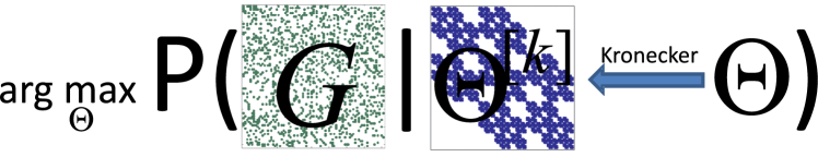
Figure 11: Kronecker parameter estimation as an optimization problem. We search over the initiator matrices ${\Theta}$ ($\equiv{\cal P}_{1}$). Using Kronecker multiplication we create probabilistic adjacency matrix ${\Theta}^{[k]}$ that is of same size as real network $G$. Now, we evaluate the likelihood by simultaneously traversing and multiplying entries of $G$ and ${\Theta}^{[k]}$ (see Eq. 8). As shown by the figure permutation ${\sigma}$ plays an important role, as permuting rows and columns of $G$ could make it look more similar to ${\Theta}^{[k]}$ and thus increase the likelihood.

We further illustrate the process of estimating Stochastic Kronecker initiator matrix ${\Theta}$ in Figure 11. We search over initiator matrices ${\Theta}$ to find the one that maximizes the likelihood $P({G}|{\Theta})$. To estimate $P({G}|{\Theta})$ we are given a concrete ${\Theta}$ and now we use Kronecker multiplication to create probabilistic adjacency matrix ${\Theta}^{[k]}$ that is of same size as real network $G$. Now, we evaluate the likelihood by traversing the corresponding entries of $G$ and ${\Theta}^{[k]}$. Equation 8 basically traverses the adjacency matrix of ${G}$, and maps every entry $(u,v)$ of $G$ to a corresponding entry $({\sigma}_{u},{\sigma}_{v})$ of ${\cal P}$. Then in case that edge $(u,v)$ exists in $G$ (i.e., ${G}[u,v]=1$) the likelihood that particular edge existing is ${\cal P}[{\sigma}_{u},{\sigma}_{v}]$, and similarly, in case the edge $(u,v)$ does not exist the likelihood is simply $1-{\cal P}[{\sigma}_{u},{\sigma}_{v}]$. This also demonstrates the importance of permutation ${\sigma}$, as permuting rows and columns of $G$ could make the adjacency matrix look more “similar” to ${\Theta}^{[k]}$, and would increase the likelihood.

So far we showed how to assess the quality (likelihood) of a particular ${\Theta}$. So, naively one could perform some kind of grid search to find best ${\Theta}$. However, this is very inefficient. A better way of doing it is to compute the gradient of the log-likelihood $\frac{\partial}{\partial{\Theta}}l({\Theta})$, and then use the gradient to update the current estimate of ${\Theta}$ and move towards a solution of higher likelihood. Algorithm 1 gives an outline of the optimization procedure.

However, there are several difficulties with this algorithm. First, we are assuming gradient descent type optimization will find a good solution, i.e., the problem does not have (too many) local minima. Second, we are summing over exponentially many permutations in equation 7. Third, the evaluation of equation 8 as it is written now takes $O(N^{2})$ time and needs to be evaluated $N!$ times. So, given a concrete ${\Theta}$ just naively calculating the likelihood takes $O(N!N^{2})$ time, and then one also has to optimize over ${\Theta}$.

Observation 2

The complexity of calculating the likelihood $P({G}|{\Theta})$ of the graph ${G}$ naively is $O(N!N^{2})$, where $N$ is the number of nodes in ${G}$.

Next, we show that all this can be done in linear time.

5.3 Summing over the node labelings

To maximize equation 6 using algorithm 1 we need to obtain the gradient of the log-likelihood $\frac{\partial}{\partial{\Theta}}l({\Theta})$. We can write:

$$\frac{\partial}{\partial{\Theta}}l({\Theta}) = \frac{\sum_{\sigma}\frac{\partial}{\partial{\Theta}}P(G|{\sigma},{\Theta})P({\sigma})}{\sum_{{\sigma}^{\prime}}P(G|{\sigma}^{\prime},{\Theta})P({\sigma}^{\prime})}$$ (9)

$$= \frac{\sum_{\sigma}\dfrac{\partial\log P(G|{\sigma},{\Theta})}{\partial{\Theta}}P({G}|{\sigma},{\Theta})P({\sigma})}{P(G|{\Theta})}$$

$$= \sum_{\sigma}\frac{\partial\log P({G}|{\sigma},{\Theta})}{\partial{\Theta}}P({\sigma}|{G},{\Theta})$$

input : size of parameter matrix ${N}_{1}$, graph ${G}$ on $N={N}_{1}^{k}$ nodes, and learning rate $\lambda$

output : MLE parameters $\hat{\Theta}$ (${N}_{1}\times{N}_{1}$ probability matrix)

initialize $\hat{\Theta}_{1}$

while not converged do evaluate gradient: $\frac{\partial}{\partial\hat{\Theta}_{t}}l(\hat{\Theta}_{t})$

update parameter estimates: $\hat{\Theta}_{t+1}=\hat{\Theta}_{t}+\lambda\frac{\partial}{\partial\hat{\Theta}_{t}}l(\hat{\Theta}_{t})$

end return $\hat{\Theta}=\hat{\Theta}_{t}$

Algorithm 1 KronFit algorithm.

3

3

3

Note we are still summing over all $N!$ permutations ${\sigma}$, so calculating Eq. 9 is computationally intractable for graphs with more than a handful of nodes. However, the equation has a nice form which allows for use of simulation techniques to avoid the summation over super-exponentially many node correspondences. Thus, we simulate draws from the permutation distribution $P({\sigma}|{G},{\Theta})$, and then evaluate the quantities at the sampled permutations to obtain the expected values of log-likelihood and gradient. Algorithm 2 gives the details.

Note that we can also permute the rows and columns of the parameter matrix ${\Theta}$ to obtain equivalent estimates. Therefore ${\Theta}$ is not strictly identifiable exactly because of these permutations. Since the space of permutations on $N$ nodes is very large (grows as $N!$) the permutation sampling algorithm will explore only a small fraction of the space of all permutations and may converge to one of the global maxima (but may not explore all ${N}_{1}!$ of them) of the parameter space. As we empirically show later our results are not sensitive to this and multiple restarts result in equivalent (but often permuted) parameter estimates.

input : Parameter matrix ${\Theta}$, and graph ${G}$

output : Log-likelihood $l({\Theta})$, and gradient $\frac{\partial}{\partial{\Theta}}l({\Theta})$

for t := 1 to T do ${\sigma}_{t}$ := SamplePermutation (${G},{\Theta}$)

$l_{t}=\log P({G}|{\sigma}^{(t)},{\Theta})$

${\textrm{g}rad}_{t}$ := $\frac{\partial}{\partial{\Theta}}\log P({G}|{\sigma}^{(t)},{\Theta})$

end return $l({\Theta})=\frac{1}{T}\sum_{t}l_{t}$, and $\frac{\partial}{\partial{\Theta}}l({\Theta})=\frac{1}{T}\sum_{t}{\textrm{g}rad}_{t}$

Algorithm 2 Calculating log-likelihood and gradient

3

3

3

5.3.1 Sampling permutations

Next, we describe the Metropolis algorithm to simulate draws from the permutation distribution $P({\sigma}|{G},{\Theta})$, which is given by

$$P({\sigma}|{G},{\Theta})=\frac{P({\sigma},{G},{\Theta})}{\sum_{\tau}P(\tau,{G},{\Theta})}=\frac{P({\sigma},{G},{\Theta})}{Z}$$

where $Z$ is the normalizing constant that is hard to compute since it involves the sum over $N!$ elements. However, if we compute the likelihood ratio between permutations ${\sigma}$ and ${\sigma}^{\prime}$ (Equation 10) the normalizing constants nicely cancel out:

$$\frac{P({\sigma}^{\prime}|{G},{\Theta})}{P({\sigma}|{G},{\Theta})} = \prod_{(u,v)\in{G}}\frac{{\cal P}[{\sigma}_{u},{\sigma}_{v}]}{{\cal P}[{\sigma}^{\prime}_{u},{\sigma}^{\prime}_{v}]}\prod_{(u,v)\notin{G}}\frac{(1-{\cal P}[{\sigma}_{u},{\sigma}_{v}])}{(1-{\cal P}[{\sigma}^{\prime}_{u},{\sigma}^{\prime}_{v}])}$$ (10)

$$= \prod_{\begin{subarray}{c}(u,v)\in{G}\\ ({\sigma}_{u},{\sigma}_{v})\neq({\sigma}^{\prime}_{u},{\sigma}^{\prime}_{v})\end{subarray}}\frac{{\cal P}[{\sigma}_{u},{\sigma}_{v}]}{{\cal P}[{\sigma}^{\prime}_{u},{\sigma}^{\prime}_{v}]}\prod_{\begin{subarray}{c}(u,v)\notin{G}\\ ({\sigma}_{u},{\sigma}_{v})\neq({\sigma}^{\prime}_{u},{\sigma}^{\prime}_{v})\end{subarray}}\frac{(1-{\cal P}[{\sigma}_{u},{\sigma}_{v}])}{(1-{\cal P}[{\sigma}^{\prime}_{u},{\sigma}^{\prime}_{v}])}$$ (11)

This immediately suggests the use of a Metropolis sampling algorithm Gamerman (1997) to simulate draws from the permutation distribution since Metropolis is solely based on such ratios (where normalizing constants cancel out). In particular, suppose that in the Metropolis algorithm (Algorithm 3) we consider a move from permutation ${\sigma}$ to a new permutation ${\sigma}^{\prime}$. Probability of accepting the move to ${\sigma}^{\prime}$ is given by Equation 10 (if $\frac{P({\sigma}^{\prime}|{G},{\Theta})}{P({\sigma}|{G},{\Theta})}\leq 1$) or 1 otherwise.

input : Kronecker initiator matrix ${\Theta}$ and a graph ${G}$ on $N$ nodes

output : Permutation ${\sigma}^{(i)}\sim P({\sigma}|{G},{\Theta})$

${\sigma}^{(0)}:=(1,\dots,N)$

$i=1$

repeat Draw $j$ and $k$ uniformly from $(1,\dots,N)$

${\sigma}^{(i)}$ := SwapNodes(${\sigma}^{(i-1)}$, $j$, $k$)

Draw $u$ from $U(0,1)$

if $u>\frac{P({\sigma}^{(i)}|{G},{\Theta})}{P({\sigma}^{(i-1)}|{G},{\Theta})}$ then ${\sigma}^{(i)}:={\sigma}^{(i-1)}$ end i = i + 1

until ${\sigma}^{(i)}\sim P({\sigma}|{G},{\Theta})$

return ${\sigma}^{(i)}$

Where $U(0,1)$ is a uniform distribution on $[0,1]$, and ${\sigma}^{\prime}$ := SwapNodes(${\sigma},j,k$) is the permutation ${\sigma}^{\prime}$ obtained from ${\sigma}$ by swapping elements at positions $j$ and $k$.

Algorithm 3 SamplePermutation(${G},{\Theta}$): Metropolis sampling of the node permutation.

9

9

9

9

9

9

9

9

9

Now we have to devise a way to sample permutations ${\sigma}$ from the proposal distribution. One way to do this would be to simply generate a random permutation ${\sigma}^{\prime}$ and then check the acceptance condition. This would be very inefficient as we expect the distribution $P({\sigma}|{G},{\Theta})$ to be heavily skewed, i.e., there will be a relatively small number of good permutations (node mappings). Even more so as the degree distributions in real networks are skewed there will be many bad permutations with low likelihood, and few good ones that do a good job in matching nodes of high degree.

To make the sampling process “smoother”, i.e., sample permutations that are not that different (and thus are not randomly jumping across the permutation space) we design a Markov chain. The idea is to stay in high likelihood part of the permutation space longer. We do this by making samples dependent, i.e., given ${\sigma}^{\prime}$ we want to generate next candidate permutation ${\sigma}^{\prime\prime}$ to then evaluate the likelihood ratio. When designing the Markov chain step one has to be careful so that the proposal distribution satisfies the detailed balance condition: $\pi({\sigma}^{\prime})P({\sigma}^{\prime}|{\sigma}^{\prime\prime})=\pi({\sigma}^{\prime\prime})P({\sigma}^{\prime\prime}|{\sigma}^{\prime})$, where $P({\sigma}^{\prime}|{\sigma}^{\prime\prime})$ is the transition probability of obtaining permutation ${\sigma}^{\prime}$ from ${\sigma}^{\prime\prime}$ and, $\pi({\sigma}^{\prime})$ is the stationary distribution.

In Algorithm 3 we use a simple proposal where given permutation ${\sigma}^{\prime}$ we generate ${\sigma}^{\prime\prime}$ by swapping elements at two uniformly at random chosen positions of ${\sigma}^{\prime}$. We refer to this proposal as SwapNodes. While this is simple and clearly satisfies the detailed balance condition it is also inefficient in a way that most of the times low degree nodes will get swapped (a direct consequence of heavy tailed degree distributions). This has two consequences, (a) we will slowly converge to good permutations (accurate mappings of high degree nodes), and (b) once we reach a good permutation, very few permutations will get accepted as most proposed permutations ${\sigma}^{\prime}$ will swap low degree nodes (as they form the majority of nodes).

A possibly more efficient way would be to swap elements of ${\sigma}$ biased based on corresponding node degree, so that high degree nodes would get swapped more often. However, doing this directly does not satisfy the detailed balance condition. A way of sampling labels biased by node degrees that at the same time satisfies the detailed balance condition is the following: we pick an edge in ${G}$ uniformly at random and swap the labels of the nodes at the edge endpoints. Notice this is biased towards swapping labels of nodes with high degrees simply as they have more edges. The detailed balance condition holds as edges are sampled uniformly at random. We refer to this proposal as SwapEdgeEndpoints.

However, the issue with this proposal is that if the graph ${G}$ is disconnected, we will only be swapping labels of nodes that belong to the same connected component. This means that some parts of the permutation space will never get visited. To overcome this problem we execute SwapNodes with some probability $\omega$ and SwapEdgeEndpoints with probability $1-\omega$.

To summarize we consider the following two permutation proposal distributions:

• ${\sigma}^{\prime\prime}=$ SwapNodes$({\sigma}^{\prime})$: we obtain ${\sigma}^{\prime\prime}$ by taking ${\sigma}^{\prime}$, uniformly at random selecting a pair of elements and swapping their positions.

• ${\sigma}^{\prime\prime}=$ SwapEdgeEndpoints$({\sigma}^{\prime})$: we obtain ${\sigma}^{\prime\prime}$ from ${\sigma}^{\prime}$ by first sampling an edge $(j,k)$ from ${G}$ uniformly at random, then we take ${\sigma}^{\prime}$ and swap the labels at positions $j$ and $k$.

5.3.2 Speeding up the likelihood ratio calculation

We further speed up the algorithm by using the following observation. As written the equation 10 takes $O(N^{2})$ to evaluate since we have to consider $N^{2}$ possible edges. However, notice that permutations ${\sigma}$ and ${\sigma}^{\prime}$ differ only at two positions, i.e. elements at position $j$ and $k$ are swapped, i.e., ${\sigma}$ and ${\sigma}^{\prime}$ map all nodes except the two to the same locations. This means those elements of equation 10 cancel out. Thus to update the likelihood we only need to traverse two rows and columns of matrix ${\cal P}$, namely rows and columns $j$ and $k$, since everywhere else the mapping of the nodes to the adjacency matrix is the same for both permutations. This gives equation 11 where the products now range only over the two rows/columns of ${\cal P}$ where ${\sigma}$ and ${\sigma}^{\prime}$ differ.

Graphs we are working with here are too large to allow us to explicitly create and store the stochastic adjacency matrix ${\cal P}$ by Kronecker powering the initiator matrix ${\Theta}$. Every time probability ${\cal P}[i,j]$ of edge $(i,j)$ is needed the equation 5 is evaluated, which takes $O(k)$. So a single iteration of Algorithm 3 takes $O(kN)$.

Observation 3

Sampling a permutation ${\sigma}$ from $P({\sigma}|{G},{\Theta})$ takes $O(kN)$.

This is gives us an improvement over the $O(N!)$ complexity of summing over all the permutations. So far we have shown how to obtain a permutation but we still need to evaluate the likelihood and find the gradients that will guide us in finding good initiator matrix. The problem here is that naively evaluating the network likelihood (gradient) as written in equation 9 takes time $O(N^{2})$. This is exactly what we investigate next and how to calculate the likelihood in linear time.

5.4 Efficiently approximating likelihood and gradient

We just showed how to efficiently sample node permutations. Now, given a permutation we show how to efficiently evaluate the likelihood and it’s gradient. Similarly as evaluating the likelihood ratio, naively calculating the log-likelihood $l({\Theta})$ or its gradient $\frac{\partial}{\partial{\Theta}}l({\Theta})$ takes time quadratic in the number of nodes. Next, we show how to compute this in linear time $O(E)$.

We begin with the observation that real graphs are sparse, which means that the number of edges is not quadratic but rather almost linear in the number of nodes, $E\ll N^{2}$. This means that majority of entries of graph adjacency matrix are zero, i.e., most of the edges are not present. We exploit this fact. The idea is to first calculate the likelihood (gradient) of an empty graph, i.e., a graph with zero edges, and then correct for the edges that actually appear in $G$.

To naively calculate the likelihood for an empty graph one needs to evaluate every cell of graph adjacency matrix. We consider Taylor approximation to the likelihood, and exploit the structure of matrix ${\cal P}$ to devise a constant time algorithm.

First, consider the second order Taylor approximation to log-likelihood of an edge that succeeds with probability $x$ but does not appear in the graph:

$$\log(1-x)\approx-x-\frac{1}{2}x^{2}$$

Calculating $l_{e}({\Theta})$, the log-likelihood of an empty graph, becomes:

$$l_{e}({\Theta})=\sum_{i=1}^{N}\sum_{j=1}^{N}\log(1-{p_{{ij}}})\approx-\bigg{(}\sum_{i=1}^{{N}_{1}}\sum_{j=1}^{{N}_{1}}{\theta_{{ij}}}\bigg{)}^{k}-\frac{1}{2}\bigg{(}\sum_{i=1}^{{N}_{1}}\sum_{j=1}^{{N}_{1}}{\theta_{{ij}}}^{2}\bigg{)}^{k}$$ (12)

Notice that while the first pair of sums ranges over $N$ elements, the last pair only ranges over ${N}_{1}$ elements (${N}_{1}=\log_{k}N$). Equation 12 holds due to the recursive structure of matrix ${\cal P}$ generated by the Kronecker product. We substitute the $\log(1-{p_{{ij}}})$ with its Taylor approximation, which gives a sum over elements of ${\cal P}$ and their squares. Next, we notice the sum of elements of ${\cal P}$ forms a multinomial series, and thus $\sum_{i,j}{p_{{ij}}}=(\sum_{i,j}{\theta_{{ij}}})^{k}$, where ${\theta_{{ij}}}$ denotes an element of ${\Theta}$, and ${p_{{ij}}}$ element of ${\Theta}^{[k]}$.

Calculating log-likelihood of ${G}$ now takes $O(E)$: First, we approximate the likelihood of an empty graph in constant time, and then account for the edges that are actually present in ${G}$, i.e., we subtract “no-edge” likelihood and add the “edge” likelihoods:

$$l({\Theta})=l_{e}({\Theta})+\sum_{(u,v)\in{G}}-\log(1-{\cal P}[{\sigma}_{u},{\sigma}_{v}])+\log({\cal P}[{\sigma}_{u},{\sigma}_{v}])$$

We note that by using the second order Taylor approximation to the log-likelihood of an empty graph, the error term of the approximation is $\frac{1}{3}(\sum_{i}{\theta_{{ij}}}^{3})^{k}$, which can diverge for large $k$. For typical values of initiator matrix ${\cal P}_{1}$ (that we present in Section 6.5) we note that one needs about fourth or fifth order Taylor approximation for the error of the approximation actually go to zero as $k$ approaches infinity, i.e., $\sum_{ij}{\theta_{{ij}}}^{n+1}<1$, where $n$ is the order of Taylor approximation employed.

5.5 Calculating the gradient

Calculation of the gradient of the log-likelihood follows exactly the same pattern as described above. First by using the Taylor approximation we calculate the gradient as if graph ${G}$ would have no edges. Then we correct the gradient for the edges that are present in ${G}$. As in previous section we speed up the calculations of the gradient by exploiting the fact that two consecutive permutations ${\sigma}$ and ${\sigma}^{\prime}$ differ only at two positions, and thus given the gradient from previous step one only needs to account for the swap of the two rows and columns of the gradient matrix $\partial{\cal P}/\partial{\Theta}$ to update to the gradients of individual parameters.

5.6 Determining the size of initiator matrix

The question we answer next is how to determine the right number of parameters, i.e., what is the right size of matrix ${\Theta}$? This is a classical question of model selection where there is a tradeoff between the complexity of the model, and the quality of the fit. Bigger model with more parameters usually fits better, however it is also more likely to overfit the data.

For model selection to find the appropriate value of ${N}_{1}$, the size of matrix ${\Theta}$, and choose the right tradeoff between the complexity of the model and the quality of the fit, we propose to use the Bayes Information Criterion (BIC) Schwarz (1978). Stochastic Kronecker graph model the presence of edges with independent Bernoulli random variables, where the canonical number of parameters is ${N}_{1}^{2k}$, which is a function of a lower-dimensional parameter ${\Theta}$. This is then a curved exponential family Efron (1975), and BIC naturally applies:

$$\textrm{BIC}({N}_{1})=-l(\hat{\Theta}_{{N}_{1}})+\frac{1}{2}{N}_{1}^{2}\log(N^{2})$$

where $\hat{\Theta}_{{N}_{1}}$ are the maximum likelihood parameters of the model with ${N}_{1}\times{N}_{1}$ parameter matrix, and $N$ is the number of nodes in $G$. Note that one could also additional term to the above formula to account for multiple global maxima of the likelihood space but as ${N}_{1}$ is small the additional term would make no real difference.

As an alternative to BIC one could also consider the Minimum Description Length (MDL) Rissanen (1978) principle where the model is scored by the quality of the fit plus the size of the description that encodes the model and the parameters.

6 Experiments on real and synthetic data

Next we described our experiments on a range of real and synthetic networks. We divide the experiments into several subsections. First we examine the convergence and mixing of the Markov chain of our permutation sampling scheme. Then we consider estimating the parameters of synthetic Kronecker graphs to see whether KronFit is able to recover the parameters used to generate the network. Last, we consider fitting Stochastic Kronecker graphs to large real world networks.

6.1 Permutation sampling

In our experiments we considered both synthetic and real graphs. Unless mentioned otherwise all synthetic Kronecker graphs were generated using ${\cal P}_{1}^{*}=[0.8,0.6;0.5,0.3]$, and $k=14$ which gives us a graph ${G}$ on $N=$16,384 nodes and $E=$115,741 edges. We chose this particular ${\cal P}_{1}^{*}$ as it resembles the typical initiator for real networks analyzed later in this section.

6.1.1 Convergence of the log-likelihood and the gradient

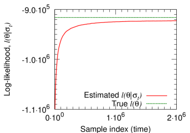
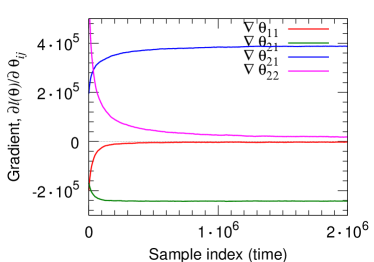
(a) Log-likelihood	(b) Gradient
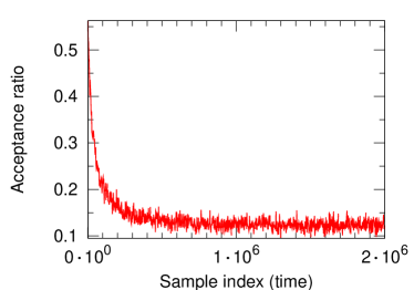
(c) Acceptance ratio	(d) Autocorrelation

Figure 12: Convergence of the log-likelihood and components of the gradient towards their true values for Metropolis permutation sampling (Algorithm 3) with the number of samples.

First, we examine the convergence of Metropolis permutation sampling, where permutations are sampled sequentially. A new permutation is obtained by modifying the previous one which creates a Markov chain. We want to assess the convergence and mixing of the chain. We aim to determine how many permutations one needs to draw to reliably estimate the likelihood and the gradient, and also how long does it take until the samples converge to the stationary distribution. For the experiment we generated a synthetic Stochastic Kronecker graphs using ${\cal P}_{1}^{*}$ as defined above. Then, starting with a random permutation we run Algorithm 3, and measure how the likelihood and the gradients converge to their true values.

In this particular case, we first generated a Stochastic Kronecker graphs ${G}$ as described above, but then calculated the likelihood and the parameter gradients for ${\Theta}^{\prime}=[0.8,0.75;0.45,0.3]$. We average the likelihoods and gradients over buckets of 1,000 consecutive samples, and plot how the log-likelihood calculated over the sampled permutations approaches the true log-likelihood (that we can compute since ${G}$ is a Stochastic Kronecker graphs).

First, we present experiments that aim to answer how many samples (i.e., permutations) does one need to draw to obtain a reliable estimate of the gradient (see Equation 9). Figure 12(a) shows how the estimated log-likelihood approaches the true likelihood. Notice that estimated values quickly converge to their true values, i.e., Metropolis sampling quickly moves towards “good” permutations. Similarly, Figure 12(b) plots the convergence of the gradients. Notice that ${\theta_{{11}}}$ and ${\theta_{{22}}}$ of ${\Theta}^{\prime}$ and ${\cal P}_{1}^{*}$ match, so gradients of these two parameters should converge to zero and indeed they do. On the other hand, ${\theta_{{12}}}$ and ${\theta_{{21}}}$ differ between ${\Theta}^{\prime}$ and ${\cal P}_{1}^{*}$. Notice, the gradient for one is positive as the parameter ${\theta_{{12}}}$ of ${\Theta}^{\prime}$ should be decreased, and similarly for ${\theta_{{21}}}$ the gradient is negative as the parameter value should be increased to match the ${\Theta}^{\prime}$. In summary, this shows that log-likelihood and gradients rather quickly converge to their true values.

In Figures 12(c) and (d) we also investigate the properties of the Markov Chain Monte Carlo sampling procedure, and assess convergence and mixing criteria. First, we plot the fraction of accepted proposals. It stabilizes at around 15%, which is quite close to the rule-of-a-thumb of 25%. Second, Figure 12(d) plots the autocorrelation of the log-likelihood as a function of the lag. Autocorrelation $r_{k}$ of a signal $X$ is a function of the lag $k$ where $r_{k}$ is defined as the correlation of signal $X$ at time $t$ with $X$ at $t+k$, i.e., correlation of the signal with itself at lag $k$. High autocorrelations within chains indicate slow mixing and, usually, slow convergence. On the other hand fast decay of autocorrelation implies better the mixing and thus one needs less samples to accurately estimate the gradient or the likelihood. Notice the rather fast autocorrelation decay.

All in all, these experiments show that one needs to sample on the order of tens of thousands of permutations for the estimates to converge. We also verified that the variance of the estimates is sufficiently small. In our experiments we start with a random permutation and use long burn-in time. Then when performing optimization we use the permutation from the previous step to initialize the permutation at the current step of the gradient descent. Intuitively, small changes in parameter space ${\Theta}$ also mean small changes in $P({\sigma}|G,{\Theta})$ .

6.1.2 Different proposal distributions

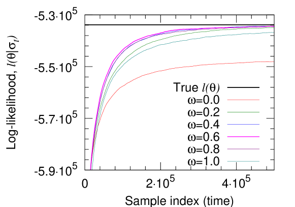
Figure 13: Convergence of the log-likelihood and gradients for Metropolis permutation sampling (Algorithm 3) for different choices of $\omega$ that interpolates between the SwapNodes ($\omega=1$) and SwapEdgeEndpoints ($\omega=0$) permutation proposal distributions. Notice fastest convergence of log-likelihood for $\omega=0.6$.

In section 5.3.1 we defined two permutation sampling strategies: SwapNodes where we pick two nodes uniformly at random and swap their labels (node ids), and SwapEdgeEndpoints where we pick a random edge in a graph and then swap the labels of the edge endpoints. We also discussed that one can interpolate between the two strategies by executing SwapNodes with probability $\omega$, and SwapEdgeEndpoints with probability $1-\omega$.

So, given a Stochastic Kronecker graphs ${G}$ on $N=$16,384 and $E=$115,741 generated from ${\cal P}_{1}^{*}=[0.8,0.7;0.5,0.3]$ we evaluate the likelihood of ${\Theta}^{\prime}=[0.8,0.75;0.45,0.3]$. As we sample permutations we observe how the estimated likelihood converges to the true likelihood. Moreover we also vary parameter $\omega$ which interpolates between the two permutation proposal distributions. The quicker the convergence towards the true log-likelihood the better the proposal distribution.

Figure 13 plots the convergence of the log-likelihood with the number of sampled permutations. We plot the average over non-overlapping buckets of 1,000 consecutive permutations. Faster convergence implies better permutation proposal distribution. When we use only SwapNodes ($\omega=1$) or SwapEdgeEndpoints ($\omega=0$) convergence is rather slow. We obtain best convergence for $\omega$ around $0.6$.

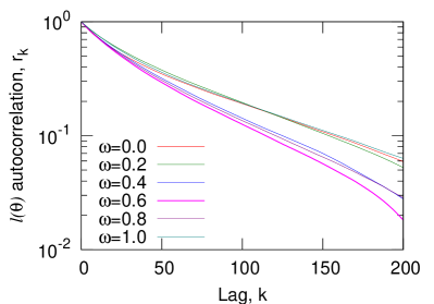
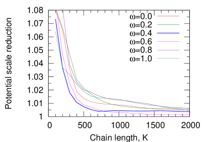
(a) Autocorrelation	(b) Potential scale reduction

Figure 14: (a) Autocorrelation plot of the log-likelihood for the different choices of parameter $\omega$. Notice we get best mixing with $\omega\approx 0.6$. (b) The potential scale reduction that compares the variance inside- and across- independent Markov chains for different values of parameter $\omega$.

Similarly, Figure 14(a) plots the autocorrelation as a function of the lag $k$ for different choices of $\omega$. Faster autocorrelation decay means better mixing of the Markov chain. Again, notice that we get best mixing for $\omega\approx 0.6$. (Notice logarithmic y-axis.)

Last, we diagnose how long the sampling procedure must be run before the generated samples can be considered to be drawn (approximately) from the stationary distribution. We call this the burn-in time of the chain. There are various procedures for assessing convergence. Here we adopt the approach of Gelman et al. Gelman et al. (2003), that is based on running multiple Markov chains each from a different starting point, and then comparing the variance within the chain and between the chains. The sooner the within- and between-chain variances become equal the shorter the burn-in time, i.e., the sooner the samples are drawn from the stationary distribution.

Let $l$ be the parameter that is being simulated with $J$ different chains, and then let $l^{(k)}_{j}$ denote the $k^{th}$ sample of the $j^{th}$ chain, where $j=1,\ldots,J$ and $k=1,\ldots,K$. More specifically, in our case we run separate permutation sampling chains. So, we first sample permutation $\sigma^{(k)}_{j}$ and then calculate the corresponding log-likelihood $l^{(k)}_{j}$.

First, we compute between and within chain variances $\hat{\sigma}^{2}_{B}$ and $\hat{\sigma}^{2}_{W}$, where between-chain variance is obtained by

$$\hat{\sigma}^{2}_{B}=\frac{K}{J-1}\sum^{J}_{j=1}(\bar{l}_{\cdot j}-\bar{l}_{\cdot\cdot})^{2}$$

where $\bar{l}_{\cdot j}=\frac{1}{K}\sum^{K}_{k=1}l^{(k)}_{j}$ and $\bar{l}_{\cdot\cdot}=\frac{1}{J}\sum^{J}_{j=1}\bar{l}_{\cdot j}$

Similarly the within-chain variance is defined by

$$\hat{\sigma}^{2}_{W}=\frac{1}{J(K-1)}\sum^{J}_{j=1}\sum^{K}_{k=1}(l_{j}^{(k)}-\bar{l}_{\cdot j})^{2}$$

Then, the marginal posterior variance of $\hat{l}$ is calculated using

$$\hat{\sigma}^{2}=\frac{K-1}{K}\hat{\sigma}^{2}_{W}+\frac{1}{K}\hat{\sigma}^{2}_{B}$$

And, finally, we estimate the potential scale reduction Gelman et al. (2003) of $l$ by

$$\sqrt{\hat{R}}=\sqrt{\frac{\hat{\sigma}^{2}}{\hat{\sigma}_{W}^{2}}}$$

Note that as the length of the chain $K\rightarrow\infty$, $\sqrt{\hat{R}}$ converges to 1 from above. The recommendation for convergence assessment from Gelman et al. (2003) is that the potential scale reduction is below $1.2$.

Figure 14(b) gives the Gelman-Rubin-Brooks plot, where we plot the potential scale reduction $\sqrt{\hat{R}}$ over the increasing chain length $K$ for different choices of parameter $\omega$. Notice that the potential scale reduction quickly decays towards 1. Similarly as in Figure 14 the extreme values of $\omega$ give slow decay, while we obtain the fastest potential scale reduction when $\omega\approx 0.6$.

6.1.3 Properties of the permutation space

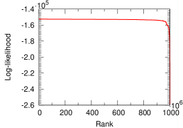
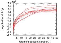
(a) $l({\Theta}|{\sigma}_{i})$ where	(b) $l({\Theta}|{\sigma}_{i})$ where	(c) $l({\Theta}_{t})$ for 10 random
${\sigma}_{i}\sim P({\sigma})$	${\sigma}_{i}\sim P({\sigma}|{\Theta},G)$	gradient descent runs

Figure 15: (a) Distribution of log-likelihood of permutations sampled uniformly at random, and (b) when sampled from $P({\sigma}|{\Theta},G)$. Notice the space of good permutations is rather small but our sampling quickly finds permutations of high likelihood. (c) Convergence of log-likelihood for 10 runs of gradient descent, each from a different random starting point.

Next we explore the properties of the permutation space. We would like to quantify what fraction of permutations are “good” (have high likelihood), and how quickly are they discovered. For the experiment we took a real network $G$ (As-RouteViews network) and the MLE parameters $\hat{\Theta}$ for it that we estimated before hand ($l(\hat{\Theta})\approx-$150,000). The network $G$ has 6,474 nodes which means the space of all permutations has $\approx 10^{22,000}$ elements.

First, we sampled 1 billion ($10^{9}$) permutations ${\sigma}_{i}$ uniformly at random, i.e., $P({\sigma}_{i})=$ 1/(6,474!) and for each evaluated its log-likelihood $l(\sigma_{i}|{\Theta})=\log P({\Theta}|G,\sigma_{i})$. We ordered the permutations in deceasing log-likelihood and plotted $l(\sigma_{i}|{\Theta})$ vs. rank. Figure 15(a) gives the plot. Notice that very few random permutations are very bad (i.e., they give low likelihood), similarly few permutations are very good, while most of them are somewhere in between. Notice that best “random” permutation has log-likelihood of $\approx-$320,000, which is far below true likelihood $l(\hat{\Theta})\approx-$150,000. This suggests that only a very small fraction of all permutations gives good node labelings.

On the other hand, we also repeated the same experiment but now using permutations sampled from the permutation distribution ${\sigma}_{i}\sim P({\sigma}|{\Theta},G)$ via our Metropolis sampling scheme. Figure 15(b) gives the plot. Notice the radical difference. Now the $l(\sigma|{\Theta}_{i})$ very quickly converges to the true likelihood of $\approx-150,000$. This suggests that while the number of “good” permutations (accurate node mappings) is rather small, our sampling procedure quickly converges to the “good” part of the permutation space where node mappings are accurate, and spends the most time there.

6.2 Properties of the optimization space

In maximizing the likelihood we use a stochastic approximation to the gradient. This adds variance to the gradient and makes efficient optimization techniques, like conjugate gradient, highly unstable. Thus we use gradient descent, which is slower but easier to control. First, we make the following observation:

Observation 4

Given a real graph ${G}$ then finding the maximum likelihood Stochastic Kronecker initiator matrix $\hat{\Theta}$

$$\hat{\Theta}=\arg\max_{{\Theta}}P({G}|{\Theta})$$

is a non-convex optimization problem.

Proof  By definition permutations of the Kronecker graphs initiator matrix ${\Theta}$ all have the same log-likelihood. This means that we have several global minima that correspond to permutations of parameter matrix ${\Theta}$, and then between them the log-likelihood drops. This means that the optimization problem is non-convex.  

The above observation does not seem promising for estimating $\hat{\Theta}$ using gradient descent as it is prone to finding local minima. To test for this behavir we run the following experiment: we generated 100 synthetic Kronecker graphs on 16,384 ($2^{14}$) nodes and 1.4 million edges on the average, each with a randomly chosen $2\times 2$ parameter matrix ${\Theta}^{*}$. For each of the 100 graphs we run a single trial of gradient descent starting from a random parameter matrix ${\Theta}^{\prime}$, and try to recover ${\Theta}^{*}$. In 98% of the cases the gradient descent converged to the true parameters. Many times the algorithm converged to a different global minima, i.e., $\hat{\Theta}$ is a permuted version of original parameter matrix ${\Theta}^{*}$. Moreover, the median number of gradient descent iterations was only 52.

This suggests surprisingly nice structure of our optimization space: it seems to behave like a convex optimization problem with many equivalent global minima. Moreover, this experiment is also a good sanity check as it shows that given a Kronecker graph we can recover and identify the parameters that were used to generate it.

Moreover, Figure 15(c) plots the log-likelihood $l({\Theta}_{t})$ of the current parameter estimate ${\Theta}_{t}$ over the iterations $t$ of the stochastic gradient descent. We plot the log-likelihood for 10 different runs of gradient descent, each time starting from a different random set of parameters ${\Theta}_{0}$. Notice that in all runs gradient descent always converges towards the optimum, and none of the runs gets stuck in some local maxima.

6.3 Convergence of the graph properties

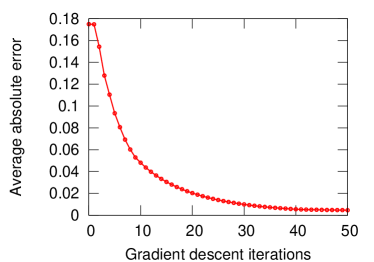
(a) Log-likelihood	(b) Average error
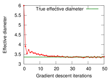
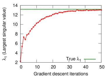
(c) Effective diameter	(d) Largest singular-value

Figure 16: Convergence of graph properties with the number of iterations of gradient descent using the synthetic dataset. We start with a random choice of parameters and with steps of gradient descent the Kronecker graph better and better matches network properties of the target graph.

We approached the problem of estimating Stochastic Kronecker initiator matrix ${\Theta}$ by defining the likelihood over the individual entries of the graph adjacency matrix. However, what we would really like is to be given a real graph ${G}$ and then generate a synthetic graph ${K}$ that has similar properties as the real ${G}$. By properties we mean network statistics that can be computed from the graph, e.g., diameter, degree distribution, clustering coefficient, etc. A priori it is not clear that our approach which tries to match individual entries of graph adjacency matrix will also be able to reproduce these global network statistics. However, as show next this is not the case.

To get some understanding of the convergence of the gradient descent in terms of the network properties we performed the following experiment. After every step $t$ of stochastic gradient descent, we compare the true graph ${G}$ with the synthetic Kronecker graph ${K}_{t}$ generated using the current parameter estimates $\hat{\Theta}_{t}$. Figure 16(a) gives the convergence of log-likelihood, and (b) gives absolute error in parameter values ($\sum|\hat{\theta}_{ij}-\theta_{ij}^{*}|$, where $\hat{\theta}_{ij}\in\hat{\Theta}_{t}$, and $\theta_{ij}^{*}\in{\Theta}^{*}$). Similarly, Figure 16(c) plots the effective diameter, and (d) gives the largest singular value of graph adjacency matrix $K$ as it converges to largest singular value of $G$.

Note how with progressing iterations of gradient descent properties of graph ${K}_{t}$ quickly converge to those of ${G}$ even though we are not directly optimizing the similarity in network properties: log-likelihood increases, absolute error of parameters decreases, diameter and largest singular value of ${K}_{t}$ both converge to ${G}$. This is a nice result as it shows that through maximizing the likelihood the resulting graphs become more and more similar also in their structural properties (even though we are not directly optimizing over them).

6.4 Fitting to real-world networks

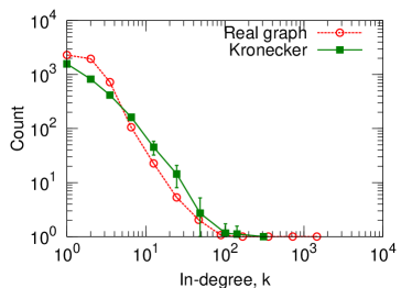
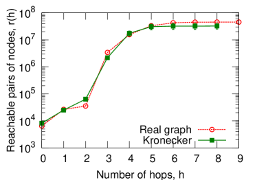
(a) Degree distribution	(b) Hop plot
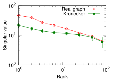
(c) Scree plot	(d) “Network” value

Figure 17: Autonomous Systems (As-RouteViews): Overlayed patterns of real graph and the fitted Kronecker graph. Notice that the fitted Kronecker graph matches patterns of the real graph while using only four parameters ($2\times 2$ initiator matrix).

Next, we present experiments of fitting Kronecker graph model to real-world networks. Given a real network $G$ we aim to discover the most likely parameters $\hat{\Theta}$ that ideally would generate a synthetic graph ${K}$ having similar properties as real $G$. This assumes that Kronecker graphs are a good model of the network structure, and that KronFit is able to find good parameters. In previous section we showed that KronFit can efficiently recover the parameters. Now we examine how well can Kronecker graph model the structure of real networks.

We consider several different networks, like a graph of connectivity among Internet Autonomous systems (As-RouteViews) with $N=$6,474 and $E=$26,467 a who-trusts-whom type social network from Epinions Richardson et al. (2003) (Epinions) with $N=$75,879 and $E=$508,960 and many others. The largest network we consider for fitting is Flickr photo-sharing online social network with 584,207 nodes and 3,555,115 edges.

For the purpose of this section we take a real network $G$, find parameters $\hat{\Theta}$ using KronFit, generate a synthetic graph ${K}$ using $\hat{\Theta}$, and then compare $G$ and ${K}$ by comparing their properties that we introduced in section 2. In all experiments we started from a random point (random initiator matrix) and run gradient descent for 100 steps. At each step we estimate the likelihood and the gradient based on 510,000 sampled permutations where we discard first 10,000 samples to allow the chain to burn-in.

6.4.1 Fitting to Autonomous Systems network

First, we focus on the Autonomous Systems network obtained from the University of Oregon Route Views project RouteViews (1997). Given the AS network $G$ we run KronFit to obtain parameter estimates $\hat{\Theta}$. Using the $\hat{\Theta}$ we then generate a synthetic Kronecker graph $K$, and compare the properties of $G$ and $K$.

Figure 17 shows properties of As-RouteViews, and compares them with the properties of a synthetic Kronecker graph generated using the fitted parameters $\hat{\Theta}$ of size $2\times 2$. Notice that properties of both graphs match really well. The estimated parameters are $\hat{\Theta}=[0.987,0.571;0.571,0.049]$.

Figure 17(a) compares the degree distributions of the As-RouteViews network and its synthetic Kronecker estimate. In this and all other plots we use the exponential binning which is a standard procedure to de-noise the data when plotting on log–log scales. Notice a very close match in degree distribution between the real graph and its synthetic counterpart.

Figure 17(b) plots the cumulative number of pairs of nodes $g(h)$ that can be reached in $\leq h$ hops. The hop plot gives a sense about the distribution of the shortest path lengths in the network and about the network diameter. Last, Figures 17(c) and (d) plot the spectral properties of the graph adjacency matrix. Figure 17(c) plots largest singular values vs. rank, and (d) plots the components of left singular vector (the network value) vs. the rank. Again notice the good agreement with the real graph while using only four parameters.

Moreover, on all plots the error bars of two standard deviations show the variance of the graph properties for different realizations $R(\hat{\Theta}^{[k]})$. To obtain the error bars we took the same $\hat{\Theta}$, and generated 50 realizations of a Kronecker graph. As for the most of the plots the error bars are so small to be practically invisible, this shows that the variance of network properties when generating a Stochastic Kronecker graph is indeed very small.

Also notice that the As-RouteViews is an undirected graph, and that the fitted parameter matrix $\hat{\Theta}$ is in fact symmetric. This means that without a priori biasing the fitting towards undirected graphs, the recovered parameters obey this aspect of the network. Fitting As-RouteViews graph from a random set of parameters, performing gradient descent for 100 iterations and at each iteration sampling half a million permutations, took less than 10 minutes on a standard desktop PC. This is a significant speedup over Bezáková et al. (2006), where by using a similar permutation sampling approach for calculating the likelihood of a preferential attachment model on similar As-RouteViews graph took about two days on a cluster of 50 machines.

6.4.2 Choice of the initiator matrix size ${N}_{1}$

${N}_{1}$	$l(\hat{\Theta})$	${N}_{1}^{k}$	${E}_{1}^{k}$	$|\{\textrm{deg}(u)>0\}|$	BIC score
2	$-$152,499	8,192	25,023	5,675	152,506
3	$-$127,066	6,561	28,790	5,683	127,083
4	$-$153,260	16,384	24,925	8,222	153,290
5	$-$149,949	15,625	29,111	9,822	149,996
6	$-$128,241	7,776	26,557	6,623	128,309
As-RouteViews			26,467	6,474

Table 2: Log-likelihood at MLE for different choices of the size of the initiator matrix ${N}_{1}$ for the As-RouteViews graph. Notice the log-likelihood $l(\hat{\theta})$ generally increases with the model complexity ${N}_{1}$. Also notice the effect of zero-padding, i.e., for ${N}_{1}=4$ and ${N}_{1}=5$ the constraint of the number of nodes being an integer power of ${N}_{1}$ decreases the log-likelihood. However, the column $|\{\textrm{deg}(u)>0\}|$ gives the number of non-isolated nodes in the network which is much less than ${N}_{1}^{k}$ and is in fact very close to the true number of nodes in the As-RouteViews. Using the BIC scores we see that ${N}_{1}=3$ or ${N}_{1}=6$ are best choices for the size of the initiator matrix.

As mentioned earlier for finding the optimal number of parameters, i.e., selecting the size of initiator matrix, BIC criterion naturally applies to the case of Kronecker graphs. Figure 23(b) shows BIC scores for the following experiment: We generated Kronecker graph with $N=$2,187 and $E=$8,736 using ${N}_{1}=3$ (9 parameters) and $k=7$. For $1\leq{N}_{1}\leq 9$ we find the MLE parameters using gradient descent, and calculate the BIC scores. The model with the lowest score is chosen. As figure 23(b) shows we recovered the true model, i.e., BIC score is the lowest for the model with the true number of parameters, ${N}_{1}=3$.

Intuitively we expect a more complex model with more parameters to fit the data better. Thus we expect larger ${N}_{1}$ to generally give better likelihood. On the other hand the fit will also depend on the size of the graph ${G}$. Kronecker graphs can only generate graphs on ${N}_{1}^{k}$ nodes, while real graphs do not necessarily have ${N}_{1}^{k}$ nodes (for some, preferably small, integers ${N}_{1}$ and $k$). To solve this problem we choose $k$ so that ${N}_{1}^{k-1}<N(G)\leq{N}_{1}^{k}$, and then augment $G$ by adding ${N}_{1}^{k}-N$ isolated nodes. Or equivalently, we pad the adjacency matrix of $G$ with zeros until it is of the appropriate size, ${N}_{1}^{k}\times{N}_{1}^{k}$. While this solves the problem of requiring the integer power of the number of nodes it also makes the fitting problem harder as when $N\ll{N}_{1}^{k}$ we are basically fitting $G$ plus a large number of isolated nodes.

Table 2 shows the results of fitting Kronecker graphs to As-RouteViews while varying the size of the initiator matrix ${N}_{1}$. First, notice that in general larger ${N}_{1}$ results in higher log-likelihood $l(\hat{\Theta})$ at MLE. Similarly, notice (column ${N}_{1}^{k}$) that while As-RouteViews has 6,474 nodes, Kronecker estimates have up to 16,384 nodes (16,384$=4^{7}$, which is the first integer power of 4 greater than 6,474). However, we also show the number of non-zero degree (non-isolated) nodes in the Kronecker graph (column $|\{\textrm{deg}(u)>0\}|$). Notice that the number of non-isolated nodes well corresponds to the number of nodes in As-RouteViews network. This shows that KronFit is actually fitting the graph well and it successfully fits the structure of the graph plus a number of isolated nodes. Last, column ${E}_{1}^{k}$ gives the number of edges in the corresponding Kronecker graph which is close to the true number of edges of the As-RouteViews graph.

Last, comparing the log-likelihood at the MLE and the BIC score in Table 2 we notice that the log-likelihood heavily dominates the BIC score. This means that the size of the initiator matrix (number of parameters) is so small that overfitting is not a concern. Thus we can just choose the initiator matrix that maximizes the likelihood. A simple calculation shows that one would need to take initiator matrices with thousands of entries before the model complexity part of BIC score would start to play a significant role.

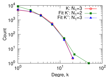
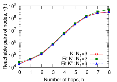
(a) Degree distribution	(b) Hop plot
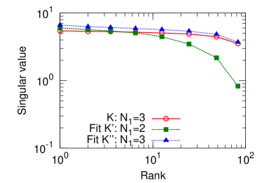
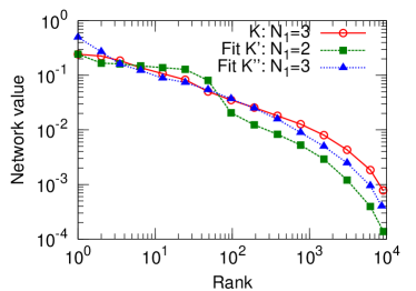
(c) Scree plot	(d) “Network” value

Figure 18: 3 by 3 Stochastic Kronecker graphs: Given a Stochastic Kronecker graphs $G$ generated from ${N}_{1}=3$ (red curve), we fit a Kronecker graph $K^{\prime}$ with ${N}_{1}^{\prime}=2$ (green) and $K^{\prime\prime}$ with ${N}_{1}^{\prime\prime}=3$ (blue). Not surprisingly $K^{\prime\prime}$ fits the properties of $K$ perfectly as the model is the of same complexity. On the other hand $K^{\prime}$ has only 4 parameters (instead of 9 as in $K$ and $K^{\prime\prime}$) and still fits well.

We further examine the sensitivity of the choice of the initiator size by the following experiment. We generate a Stochastic Kronecker graphs $K$ on 9 parameters (${N}_{1}=3$), and then fit a Kronecker graph $K^{\prime}$ with a smaller number of parameters (4 instead of 9, ${N}_{1}^{\prime}=2$). And also a Kronecker graph $K^{\prime\prime}$ of the same complexity as $K$ (${N}_{1}^{\prime\prime}=3$).

Figure 18 plots the properties of all three graphs. Not surprisingly $K^{\prime\prime}$ (blue) fits the properties of $K$ (red) perfectly as the initiator is of the same size. On the other hand $K^{\prime}$ (green) is a simpler model with only 4 parameters (instead of 9 as in $K$ and $K^{\prime\prime}$) and still generally fits well: hop plot and degree distribution match well, while spectral properties of graph adjacency matrix, especially scree plot, are not matched that well. This shows that nothing drastic happens and that even a bit too simple model still fits the data well. In general we observe empirically that by increasing the size of the initiator matrix one does not gain radically better fits for degree distribution and hop plot. On the other hand there is usually an improvement in the scree plot and the plot of network values when one increases the initiator size.

6.4.3 Network parameters over time

Snapshot at time	$N$	$E$	$l(\hat{\Theta})$	Estimates at MLE, $\hat{\Theta}$
$T_{1}$	2,048	8,794	$-$40,535	$[0.981,0.633;0.633,0.048]$
$T_{2}$	4,088	15,711	$-$82,675	$[0.934,0.623;0.622,0.044]$
$T_{3}$	6,474	26,467	$-$152,499	$[0.987,0.571;0.571,0.049]$

Table 3: Parameter estimates of the three temporal snapshots of the As-RouteViews network. Notice that estimates stay remarkably stable over time.

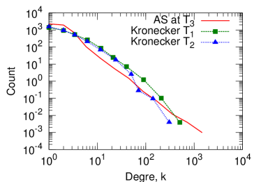
(a) Degree	(b) Hop plot
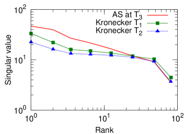
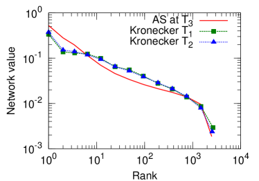
(c) Scree plot	(d) “Network” value

Figure 19: Autonomous systems network over time (As-RouteViews): Overlayed patterns of real As-RouteViews network at time $T_{3}$ and the Kronecker graphs with parameters estimated from As-RouteViews at time $T_{1}$ and $T_{2}$. Notice good fits which means that parameters estimated on historic snapshots can be used to estimate the graph in the future.

Next we briefly examine the evolution of the Kronecker initiator for a temporally evolving graph. The idea is that given parameter estimates of a real-graph $G_{t}$ at time $t$, we can forecast the future structure of the graph $G_{t+x}$ at time $t+x$, i.e., using parameters obtained from $G_{t}$ we can generate a larger synthetic graph $K$ that will be similar to $G_{t+x}$.

As we have the information about the evolution of the As-RouteViews network, we estimated parameters for three snapshots of the network when it had about $2^{k}$ nodes. Table 3 gives the results of the fitting for the three temporal snapshots of the As-RouteViews network. Notice the parameter estimates $\hat{\Theta}$ remain remarkably stable over time. This means that Kronecker graphs can be used to estimate the structure of the networks in the future, i.e., parameters estimated from the historic data can extrapolate the graph structure in the future.

Figure 19 further explores this. It overlays the graph properties of the real As-RouteViews network at time $T_{3}$ and the synthetic graphs for which we used the parameters obtained on historic snapshots of As-RouteViews at times $T_{1}$ and $T_{2}$. The agreements are good which demonstrates that Kronecker graphs can forecast the structure of the network in the future.

Moreover, this experiments also shows that parameter estimates do not suffer much from the zero padding of graph adjacency matrix (i.e., adding isolated nodes to make $G$ have ${N}_{1}^{k}$ nodes). Snapshots of As-RouteViews at $T_{1}$ and $T_{2}$ have close to $2^{k}$ nodes, while we had to add 26% (1,718) isolated nodes to the network at $T_{3}$ to make the number of nodes be $2^{k}$. Regardless of this we see the parameter estimates $\hat{\Theta}$ remain basically constant over time, which seems to be independent of the number of isolated nodes added. This means that the estimated parameters are not biased too much from zero padding the adjacency matrix of $G$.

6.5 Fitting to other large real-world networks

Network	$N$	$E$	Estimated MLE parameters $\hat{\Theta}$	$l(\hat{\Theta})$	Time
As-RouteViews	6,474	26,467	$[0.987,0.571;0.571,0.049]$	$-$152,499	8m15s
AtP-gr-qc	19,177	26,169	$[0.902,0.253;0.221,0.582]$	$-$242,493	7m40s
Bio-Proteins	4,626	29,602	$[0.847,0.641;0.641,0.072]$	$-$185,130	43m41s
Email-Inside	986	32,128	$[0.999,0.772;0.772,0.257]$	$-$107,283	1h07m
CA-gr-qc	5,242	28,980	$[0.999,0.245;0.245,0.691]$	$-$160,902	14m02s
As-Newman	22,963	96,872	$[0.954,0.594;0.594,0.019]$	$-$593,747	28m48s
Blog-nat05-6m	31,600	271,377	$[0.999,0.569;0.502,0.221]$	$-$1,994,943	47m20s
Blog-nat06all	32,443	318,815	$[0.999,0.578;0.517,0.221]$	$-$2,289,009	52m31s
CA-hep-ph	12,008	237,010	$[0.999,0.437;0.437,0.484]$	$-$1,272,629	1h22m
CA-hep-th	9,877	51,971	$[0.999,0.271;0.271,0.587]$	$-$343,614	21m17s
Cit-hep-ph	30,567	348,721	$[0.994,0.439;0.355,0.526]$	$-$2,607,159	51m26s
Cit-hep-th	27,770	352,807	$[0.990,0.440;0.347,0.538]$	$-$2,507,167	15m23s
Epinions	75,879	508,837	$[0.999,0.532;0.480,0.129]$	$-$3,817,121	45m39s
Gnutella-25	22,687	54,705	$[0.746,0.496;0.654,0.183]$	$-$530,199	16m22s
Gnutella-30	36,682	88,328	$[0.753,0.489;0.632,0.178]$	$-$919,235	14m20s
Delicious	205,282	436,735	$[0.999,0.327;0.348,0.391]$	$-$4,579,001	27m51s
Answers	598,314	1,834,200	$[0.994,0.384;0.414,0.249]$	$-$20,508,982	2h35m
CA-DBLP	425,957	2,696,489	$[0.999,0.307;0.307,0.574]$	$-$26,813,878	3h01m
Flickr	584,207	3,555,115	$[0.999,0.474;0.485,0.144]$	$-$32,043,787	4h26m
Web-Notredame	325,729	1,497,134	$[0.999,0.414;0.453,0.229]$	$-$14,588,217	2h59m

Table 4: Results of parameter estimation for 20 different networks. Table 5 gives the description and basic properties of the above network datasets. Networks are available for download at http://snap.stanford.edu.

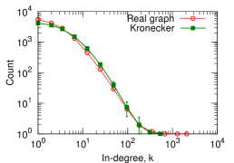
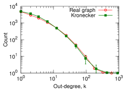
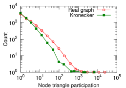
(a) In-Degree	(b) Out-degree	(c) Triangle participation
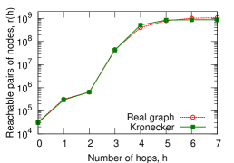
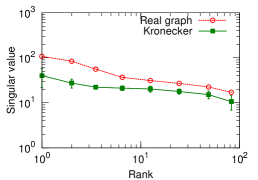
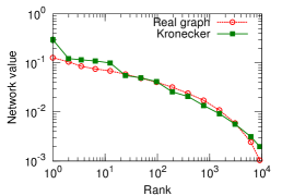
(d) Hop plot	(e) Scree plot	(f) “Network” value

Figure 20: Blog network (Blog-nat06all): Overlayed patterns of real network and the estimated Kronecker graph using 4 parameters ($2\times 2$ initiator matrix). Notice that the Kronecker graph matches all properties of the real network.

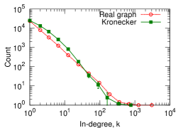
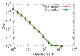
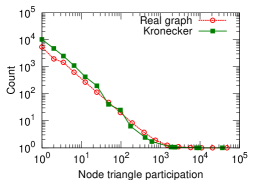
(a) In-Degree	(b) Out-degree	(c) Triangle participation
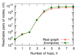
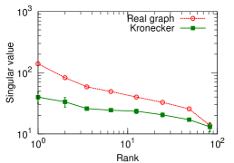
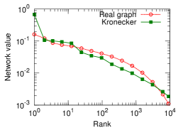
(d) Hop plot	(e) Scree plot	(f) “Network” value

Figure 21: Epinions who-trusts-whom social network: Overlayed patterns of real network and the fitted Kronecker graph using only 4 parameters ($2\times 2$ initiator matrix). Again, the synthetic Kronecker graph matches all the properties of the real network.

Last, we present results of fitting Stochastic Kronecker graphs to 20 large real-world networks: large online social networks, like Epinions, Flickr and Delicious, web and blog graphs (Web-Notredame, Blog-nat05-6m, Blog-nat06all), internet and peer-to-peer networks (As-Newman, Gnutella-25, Gnutella-30), collaboration networks of co-authorships from DBLP (CA-DBLP) and various areas of physics (CA-hep-th, CA-hep-ph, CA-gr-qc), physics citation networks (Cit-hep-ph, Cit-hep-th), an email network (Email-Inside), a protein interaction network Bio-Proteins, and a bipartite affiliation network (authors-to-papers, AtP-gr-qc). Refer to table 5 in the appendix for the description and basic properties of these networks. They are available for download at http://snap.stanford.edu.

For each dataset we started gradient descent from a random point (random initiator matrix) and ran it for 100 steps. At each step we estimate the likelihood and the gradient based on 510,000 sampled permutations where we discard first 10,000 samples to allow the chain to burn-in.

Table 4 gives the estimated parameters, the corresponding log-likelihoods and the wall clock times. All experiments were carried out on standard desktop computer. Notice that the estimated initiator matrices $\hat{\Theta}$ seem to have almost universal structure with a large value in the top left entry, a very small value at the bottom right corner and intermediate values in the other two corners. We further discuss the implications of such structure of Kronecker initiator matrix on the global network structure in next section.

Last, Figures 20 and 21 show overlays of various network properties of real and the estimated synthetic networks. In addition to the network properties we plotted in Figure 18, we also separately plot in- and out-degree distributions (as both networks are directed) and plot the node triangle participation in panel (c), where we plot the number of triangles a node participates in versus the number of such nodes. (Again the error bars show the variance of network properties over different realizations $R(\hat{\Theta}^{[k]})$ of a Stochastic Kronecker graph.)

Notice that for both networks and in all cases the properties of the real network and the synthetic Kronecker coincide really well. Using Stochastic Kronecker graphs with just 4 parameters we match the scree plot, degree distributions, triangle participation, hop plot and network values.

Given the previous experiments from the Autonomous systems graph we only present the results for the simplest model with initiator size ${N}_{1}=2$. Empirically we also observe that ${N}_{1}=2$ gives surprisingly good fits and the estimation procedure is the most robust and converges the fastest. Using larger initiator matrices ${N}_{1}>2$ generally helps improve the likelihood but not dramatically. In terms of matching the network properties we also gent a slight improvement by making the model more complex. Figure 22 gives the percent improvement in log-likelihood as we make the model more complex. We use the log-likelihood of a $2\times 2$ model as a baseline and estimate the log-likelihood at the MLE for larger initiator matrices. Again, models with more parameters tend to fit better. However, sometimes due to zero-padding of a graph adjacency matrix they actually have lower log-likelihood (as for example seen in Table 2).

Figure 22: Percent improvement in log-likelihood over the $2\times 2$ model as we increase the model complexity (size of initiator matrix). In general larger initiator matrices that have more degrees of freedom help improving the fit of the model.

6.6 Scalability

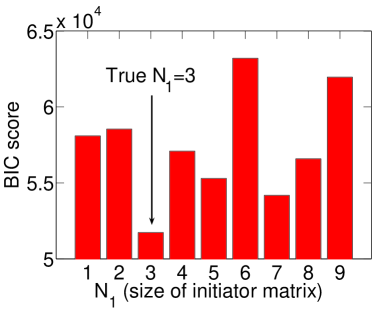
(a) Scalability	(b) Model selection

Figure 23: (a) Processor time to sample 1 million gradients as the graph grows. Notice the algorithm scales linearly with the graph size. (b) BIC score for model selection.

Last we also empirically evaluate the scalability of the KronFit. The experiment confirms that KronFit runtime scales linearly with the number of edges $E$ in a graph $G$. More precisely, we performed the following experiment.

We generated a sequence of increasingly larger synthetic graphs on $N$ nodes and $8N$ edges, and measured the time of one iteration of gradient descent, i.e., sample 1 million permutations and evaluate the gradients. We started with a graph on 1,000 nodes, and finished with a graph on 8 million nodes, and 64 million edges. Figure 23(a) shows KronFit scales linearly with the size of the network. We plot wall-clock time vs. size of the graph. The dashed line gives a linear fit to the data points.

7 Discussion

Here we discuss several of the desirable properties of the proposed Kronecker graphs.

Generality: Stochastic Kronecker graphs include several other generators as special cases: For ${\theta_{{ij}}}=c$, we obtain the classical Erdős-Rényi random graph model. For ${\theta_{{i,j}}}\in\{0,1\}$, we obtain a deterministic Kronecker graph. Setting the ${{K}}_{1}$ matrix to a $2\times 2$ matrix, we obtain the R-MAT generator Chakrabarti et al. (2004). In contrast to Kronecker graphs, the RMAT cannot extrapolate into the future, since it needs to know the number of edges to insert. Thus, it is incapable of obeying the densification power law.

Phase transition phenomena: The Erdős-Rényi graphs exhibit phase transitions Erdős and Rényi (1960). Several researchers argue that real systems are “at the edge of chaos” or phase transition Bak (1996); Sole and Goodwin (2000). Stochastic Kronecker graphs also exhibit phase transitions Mahdian and Xu (2007) for the emergence of the giant component and another phase transition for connectivity.

Implications to the structure of the large-real networks: Empirically we found that $2\times 2$ initiator (${N}_{1}=2$) fits well the properties of real-world networks. Moreover, given a $2\times 2$ initiator matrix, one can look at it as a recursive expansion of two groups into sub-groups. We introduced this recursive view of Kronecker graphs back in section 3. So, one can then interpret the diagonal values of $\Theta$ as the proportion of edges inside each of the groups, and the off-diagonal values give the fraction of edges connecting the groups. Figure 24 illustrates the setting for two groups.

For example, as shown in Figure 24, large $a,d$ and small $b,c$ would imply that the network is composed of hierarchically nested communities, where there are many edges inside each community and few edges crossing them Leskovec (2009). One could think of this structure as some kind of organizational or university hierarchy, where one expects the most friendships between people within same lab, a bit less between people in the same department, less across different departments, and the least friendships to be formed across people from different schools of the university.

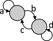
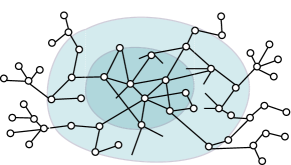
(a) $2\times 2$ initiator matrix	(b) Two recursive communities	(c) Core-periphery

Figure 24: $2\times 2$ Kronecker initiator matrix (a) can be thought of as two communities where there are $a$ and $d$ edges inside each of the communities and $b$ and $c$ edges crossing the two communities as illustrated in (b). Each community can then be recursively divided using the same pattern. (c) The onion like core-periphery structure where the network gets denser and denser as we move towards the center of the network.

However, parameter estimates for a wide range of networks presented in Table 4 suggests a very different picture of the network structure. Notice that for most networks $a\gg b>c\gg d$. Moreover, $a\approx 1$, $b\approx c\approx 0.6$ and $d\approx 0.2$. We empirically observed that the same structure of initiator matrix $\hat{\Theta}$ also holds when fitting $3\times 3$ or $4\times 4$ models. Always the top left element is the largest and then the values on the diagonal decay faster than off the diagonal Leskovec (2009).

This suggests a network structure which is also known as core-periphery Borgatti and Everett (2000); Holme (2005), the jellyfish Tauro et al. (2001); Siganos et al. (2006), or the octopus Chung and Lu (2006) structure of the network as illustrated in Figure 24(c).

All of the above basically say that the network is composed of a densely linked network core and the periphery. In our case this would imply the following structure of the initiator matrix. The core is modeled by parameter $a$ and the periphery by $d$. Most edges are inside the core (large $a$), and very few between the nodes of periphery (small $d$). Then there are many more edges between the core and the periphery than inside the periphery ($b,c>d$) Leskovec (2009). This is exactly what we see as well. And in spirit of Kronecker graphs the structure repeats recursively — the core again has the dense core and the periphery, and so on. And similarly the periphery itself has the core and the periphery.

This suggest an “onion” like nested core-periphery Leskovec et al. (2008a, b) network structure as illustrated in Figure 24(c), where the network is composed of denser and denser layers as one moves towards the center of the network. We also observe similar structure of the Kronecker initiator when fitting $3\times 3$ or $4\times 4$ initiator matrix. The diagonal elements have large but decreasing values with off diagonal elements following same decreasing pattern.

One of the implications of this is that networks do not break nicely into hierarchically organized sets of communities that lend themselves to graph partitioning and community detection algorithms. On contrary, this suggests that large networks can be decomposed into a densely linked core with many small periphery pieces hanging off the core. This is in accordance with our recent results Leskovec et al. (2008a, b), that make similar observation (but based on a completely different methodology based on graph partitioning) about the clustering and community structure of large real-world networks.

8 Conclusion

In conclusion, the main contribution of this work is a family of models of network structure that uses a non-traditional matrix operation, the Kronecker product. The resulting graphs (a) have all the static properties (heavy-tailed degree distribution, small diameter, etc.), (b) all the temporal properties (densification, shrinking diameter) that are found in real networks. And in addition, (c) we can formally prove all of these properties.

Several of the proofs are extremely simple, thanks to the rich theory of Kronecker multiplication. We also provide proofs about the diameter and effective diameter, and we show that Stochastic Kronecker graphs can mimic real graphs well.

Moreover, we also presented KronFit, a fast, scalable algorithm to estimate Stochastic Kronecker initiator, which can be then used to create a synthetic graph that mimics the properties of a given real network.

In contrast to earlier work, our work has the following novelties: (a) it is among the few that estimates the parameters of the chosen generator in a principled way, (b) it is among the few that has a concrete measure of goodness of the fit (namely, the likelihood), (c) it avoids the quadratic complexity of computing the likelihood by exploiting the properties of the Kronecker graphs, and (d) it avoids the factorial explosion of the node correspondence problem, by using the Metropolis sampling.

The resulting algorithm matches well all the known properties of real graphs, as we show with the Epinions graph and the AS graph, it scales linearly on the number of edges, and it is orders of magnitudes faster than earlier graph-fitting attempts: 20 minutes on a commodity PC, versus 2 days on a cluster of 50 workstations Bezáková et al. (2006).

The benefits of fitting a Kronecker graph model into a real graph are several:

• Extrapolation: Once we have the Kronecker generator ${\Theta}$ for a given real matrix ${G}$ (such that ${G}$ is mimicked by ${\Theta}^{[k]}$), a larger version of ${G}$ can be generated by ${\Theta}^{[k+1]}$.

• Null-model: When analyzing a real network $G$ one often needs to asses the significance of the observation. ${\Theta}^{[k]}$ that mimics $G$ can be used as an accurate model of $G$.

• Network structure: Estimated parameters give insight into the global network and community structure of the network.

• Forecasting: As we demonstrated one can obtain ${\Theta}$ from a graph $G_{t}$ at time $t$ such that ${G}$ is mimicked by ${\Theta}^{[k]}$. Then ${\Theta}$ can be used to model the structure of $G_{t+x}$ in the future.

• Sampling: Similarly, if we want a realistic sample of the real graph, we could use a smaller exponent in the Kronecker exponentiation, like ${\Theta}^{[k-1]}$.

• Anonymization: Since ${\Theta}^{[k]}$ mimics ${G}$, we can publish ${\Theta}^{[k]}$, without revealing information about the nodes of the real graph ${G}$.

Future work could include extensions of Kronecker graphs to evolving networks. We envision formulating a dynamic Bayesian network with first order Markov dependencies, where parameter matrix at time $t$ depends on the graph $G_{t}$ at current time $t$ and the parameter matrix at time $t-1$. Given a series of network snapshots one would then aim to estimate initiator matrices at individual time steps and the parameters of the model governing the evolution of the initiator matrix. We expect that based on the evolution of initiator matrix one would gain greater insight in the evolution of large networks.

Second direction for future work is to explore connections between Kronecker graphs and Random Dot Product graphs Young and Scheinerman (2007); Nickel (2008). This also nicely connects with the “attribute view” of Kronecker graphs as described in Section 3.5. It would be interesting to design methods to estimate the individual node attribute values as well as the attribute-attribute similarity matrix (i.e., the initiator matrix). As for some networks node attributes are already given one could then try to infer “hidden” or missing node attribute values and this way gain insight into individual nodes as well as individual edge formations. Moreover, this would be interesting as one could further evaluate how realistic is the “attribute view” of Kronecker graphs.

Last, we also mention possible extensions of Kronecker graphs for modeling weighted and labeled networks. Currently Stochastic Kronecker graphs use a Bernoulli edge generation model, i.e., an entry of big matrix ${\cal P}$ encodes the parameter of a Bernoulli coin. In similar spirit one could consider entries of ${\cal P}$ to encode parameters of different edge generative processes. For example, to generate networks with weights on edges an entry of ${\cal P}$ could encode the parameter of an exponential distribution, or in case of labeled networks one could use several initiator matrices in parallel and this way encode parameters of a multinomial distribution over different node attribute values.

A Table of networks

Table 5 lists all the network datasets that were used in this paper. We also computed some of the structural network properties. Most of the networks are available for download from http://snap.stanford.edu.

Network	$N$	$E$	$N_{c}$	$N_{c}/N$	$\bar{C}$	$D$	$\bar{D}$	Description
Social networks
Answers	598,314	1,834,200	488,484	0.82	0.11	22	5.72	Yahoo! Answers social network Leskovec et al. (2008a)
Delicious	205,282	436,735	147,567	0.72	0.3	24	6.28	del.icio.us social network Leskovec et al. (2008a)
Email-Inside	986	32,128	986	1.00	0.45	7	2.6	European research organization email network Leskovec et al. (2007a)
Epinions	75,879	508,837	75,877	1.00	0.26	15	4.27	Who-trusts-whom graph of epinions.com Richardson et al. (2003)
Flickr	584,207	3,555,115	404,733	0.69	0.4	18	5.42	Flickr photo sharing social network Kumar et al. (2006)
Information (citation) networks
Blog-nat05-6m	31,600	271,377	29,150	0.92	0.24	10	3.4	Blog-to-blog citation network (6 months of data) Leskovec et al. (2007b)
Blog-nat06all	32,443	318,815	32,384	1.00	0.2	18	3.94	Blog-to-blog citation network (1 year of data) Leskovec et al. (2007b)
Cit-hep-ph	30,567	348,721	34,401	1.13	0.3	14	4.33	Citation network of ArXiv hep-th papers Gehrke et al. (2003)
Cit-hep-th	27,770	352,807	27,400	0.99	0.33	15	4.2	Citations network of ArXiv hep-ph papers Gehrke et al. (2003)
Collaboration networks
CA-DBLP	425,957	2,696,489	317,080	0.74	0.73	23	6.75	DBLP co-authorship network Backstrom et al. (2006)
CA-gr-qc	5,242	28,980	4,158	0.79	0.66	17	6.1	Co-authorship network in gr-qc category of ArXiv Leskovec et al. (2005b)
CA-hep-ph	12,008	237,010	11,204	0.93	0.69	13	4.71	Co-authorship network in hep-ph category of ArXiv Leskovec et al. (2005b)
CA-hep-th	9,877	51,971	8,638	0.87	0.58	18	5.96	Co-authorship network in hep-th category of ArXiv Leskovec et al. (2005b)
Web graphs
Web-Notredame	325,729	1,497,134	325,729	1.00	0.47	46	7.22	Web graph of University of Notre Dame Albert et al. (1999)
Internet networks
As-Newman	22,963	96,872	22,963	1.00	0.35	11	3.83	AS graph from Newman new (July 16, 2007)
As-RouteViews	6,474	26,467	6,474	1.00	0.4	9	3.72	AS from Oregon Route View Leskovec et al. (2005b)
Gnutella-25	22,687	54,705	22,663	1.00	0.01	11	5.57	Gnutella P2P network on 3/25 2000 Ripeanu et al. (2002)
Gnutella-30	36,682	88,328	36,646	1.00	0.01	11	5.75	Gnutella P2P network on 3/30 2000 Ripeanu et al. (2002)
Bi-partite networks
AtP-gr-qc	19,177	26,169	14,832	0.77	0	35	11.08	Affiliation network of gr-qc category in ArXiv Leskovec et al. (2007b)
Biological networks
Bio-Proteins	4,626	29,602	4,626	1.00	0.12	12	4.24	Yeast protein interaction network Colizza et al. (2005)

Table 5: Network datasets we analyzed. Statistics of networks we consider: number of nodes $N$; number of edges $E$, number of nodes in largest connected component $N_{c}$, fraction of nodes in largest connected component $N_{c}/N$, average clustering coefficient $\bar{C}$; diameter $D$, and average path length $\bar{D}$. Networks are available for download at http://snap.stanford.edu.

References

- new (July 16, 2007) Network data. http://www-personal.umich.edu/~mejn/netdata, July 16, 2007.
- Albert and Barabási (2002) R. Albert and A.-L. Barabási. Statistical mechanics of complex networks. Reviews of Modern Physics, 74(1):47–97, 2002.
- Albert et al. (1999) R. Albert, H. Jeong, and A.-L. Barabási. Diameter of the world-wide web. Nature, 401:130–131, September 1999.
- Backstrom et al. (2006) L. Backstrom, D. Huttenlocher, J. Kleinberg, and X. Lan. Group formation in large social networks: membership, growth, and evolution. In KDD ’06: Proceedings of the 12th ACM SIGKDD international conference on Knowledge discovery and data mining, pages 44–54, 2006. ISBN 1-59593-339-5.
- Bak (1996) P. Bak. How Nature Works: The Science of Self-Organized Criticality. Springer, September 1996.
- Barabási and Albert (1999) A.-L. Barabási and R. Albert. Emergence of scaling in random networks. Science, 286:509–512, 1999.
- Barabási et al. (2001) A.-L. Barabási, E. Ravasz, and T. Vicsek. Deterministic scale-free networks. Physica A, 299:559–564, 2001.
- Bezáková et al. (2006) I. Bezáková, A. Kalai, and R. Santhanam. Graph model selection using maximum likelihood. In ICML ’06: Proceedings of the 23rd international conference on Machine learning, pages 105–112, 2006.
- Bi et al. (2001) Z. Bi, C. Faloutsos, and F. Korn. The DGX distribution for mining massive, skewed data. In KDD ’01: Proceedings of the 6th ACM SIGKDD international conference on Knowledge discovery and data mining, pages 17–26, 2001.
- Blum et al. (2006) A. Blum, H. Chan, and M. Rwebangira. A random-surfer web-graph model. In ANALCO ’06: Proceedings of the 3rd Workshop on Analytic Algorithmics and Combinatorics, 2006.
- Borgatti and Everett (2000) S. P. Borgatti and M. G. Everett. Models of core/periphery structures. Social Networks, 21(4):375–395, 2000.
- Bottreau and Metivier (1998) A. Bottreau and Y. Metivier. Some remarks on the kronecker product of graphs. Information Processing Letters, 68(2):55 – 61, 1998.
- Broder et al. (2000) A. Broder, R. Kumar, F. Maghoul, P. Raghavan, S. Rajagopalan, R. Stata, A. Tomkins, and J. Wiener. Graph structure in the web: experiments and models. In WWW ’00: Proceedings of the 9th international conference on World Wide Web, 2000.
- Bu and Towsley (2002) T. Bu and D. F. Towsley. On distinguishing between internet power law topology generators. In INFOCOM, 2002.
- Butts (2005) C. T. Butts. Permutation models for relational data. (tech. rep. mbs 05-02, Univ. of California, Irvine, 2005.
- Carlson and Doyle (1999) J. M. Carlson and J. Doyle. Highly optimized tolerance: a mechanism for power laws in designed systems. Physical Review E, 60(2):1412–1427, 1999.
- Chakrabarti et al. (2004) D. Chakrabarti, Y. Zhan, and C. Faloutsos. R-mat: A recursive model for graph mining. In SDM ’04: SIAM Conference on Data Mining, 2004.
- Chow (1997) T. Chow. The Q-spectrum and spanning trees of tensor products of bipartite graphs. Proc. Amer. Math. Soc., 125:3155–3161, 1997.
- Chung and Lu (2006) F. R. K. Chung and L. Lu. Complex Graphs and Networks, volume 107 of CBMS Regional Conference Series in Mathematics. American Mathematical Society, 2006.
- Chung et al. (2003) F. R. K. Chung, L. Lu, and V. Vu. Eigenvalues of random power law graphs. Annals of Combinatorics, 7:21–33, 2003.
- Clauset et al. (2007) A. Clauset, C. R. Shalizi, and M. E. J. Newman. Power-law distributions in empirical data. ArXiv, ArXiv:0706.1062, Jun 2007.
- Clauset et al. (2008) A. Clauset, C. Moore, and M. E. J. Newman. Hierarchical structure and the prediction of missing links in networks. Nature, 453(7191):98–101, 2008.
- Colizza et al. (2005) V. Colizza, A. Flammini, M. A. Serrano, and A. Vespignani. Characterization and modeling of protein protein interaction networks. Physica A Statistical Mechanics and its Applications, 352:1–27, 2005.
- Crovella and Bestavros (1997) M. E. Crovella and A. Bestavros. Self-similarity in World Wide Web traffic: evidence and possible causes. IEEE /ACM Transactions on Networking, 5(6):835–846, 1997.
- Dill et al. (2002) S. Dill, R. Kumar, K. S. Mccurley, S. Rajagopalan, D. Sivakumar, and A. Tomkins. Self-similarity in the web. ACM Trans. Interet Technology, 2(3):205–223, 2002. ISSN 1533-5399.
- Dorogovtsev et al. (2002) S. N. Dorogovtsev, A. V. Goltsev, and J. F. F. Mendes. Pseudofractal scale-free web. Physical Review E, 65(6):066122, Jun 2002.
- Efron (1975) B. Efron. Defining the curvature of a statistical problem (with applications to second order efficiency). Ann. Statist., 3(6):1189–1242, 1975.
- Erdős and Rényi (1960) P. Erdős and A. Rényi. On the evolution of random graphs. Publication of the Mathematical Institute of the Hungarian Acadamy of Science, 5:17–67, 1960.
- Fabrikant et al. (2002) A. Fabrikant, E. Koutsoupias, and C. H. Papadimitriou. Heuristically optimized trade-offs: A new paradigm for power laws in the internet. In ICALP ’02: Proceedings of the 29th International Colloquium on Automata, Languages, and Programming, volume 2380, 2002.
- Faloutsos et al. (1999) M. Faloutsos, P. Faloutsos, and C. Faloutsos. On power-law relationships of the internet topology. In SIGCOMM ’99: Proceedings of the conference on Applications, technologies, architectures, and protocols for computer communication, pages 251–262, 1999.
- Farkas et al. (2001) I. Farkas, I. Deréni, A.-L. Barabási, and T. Vicsek. Spectra of “real-world” graphs: beyond the semicircle law. Physical Review E, 64(026704), 2001.
- Flaxman et al. (2007) A. D. Flaxman, A. M. Frieze, and J. Vera. A geometric preferential attachment model of networks II. In WAW ’07: Proceedings of the 5th Workshop On Algorithms And Models For The Web-Graph, pages 41–55, 2007.
- Gamerman (1997) D. Gamerman. Markov chain Monte Carlo, Stochastic simulation for Bayesian inference. Chapman & Hall, London, 1997.
- Gehrke et al. (2003) J. Gehrke, P. Ginsparg, and J. M. Kleinberg. Overview of the 2003 kdd cup. SIGKDD Explorations, 5(2):149–151, 2003.
- Gelman et al. (2003) A. Gelman, J. B. Carlin, H. S. Stern, and D.B. Rubin. Bayesian Data Analysis, Second Edition. Chapman & Hall, London, July 2003. ISBN 158488388X.
- Hammack (2009) R. H. Hammack. Proof of a conjecture concerning the direct product of bipartite graphs. European Journal of Combinatorics, 30(5):1114 – 1118, 2009. ISSN 0195-6698. Part Special Issue on Metric Graph Theory.
- Holme (2005) P. Holme. Core-periphery organization of complex networks. Physical Review E, 72:046111, 2005.
- Imrich (1998) W. Imrich. Factoring cardinal product graphs in polynomial time. Discrete Mathematics, 192(1-3):119–144, 1998. ISSN 0012-365X.
- Imrich and Klavžar (2000) W. Imrich and S. Klavžar. Product Graphs: Structure and Recognition. Wiley, 2000. ISBN 1-4020-0489-3.
- Kleinberg (1999) J. M. Kleinberg. The small-world phenomenon: an algorithmic perspective. Technical Report 99-1776, Cornell Computer Science Department, 1999.
- Kleinberg et al. (1999) J. M. Kleinberg, S. R. Kumar, P. Raghavan, S. Rajagopalan, and A. Tomkins. The web as a graph: Measurements, models and methods. In COCOON ’99: Proceedings of the International Conference on Combinatorics and Computing, 1999.
- Klemm and Eguíluz (2002) K. Klemm and V. M. Eguíluz. Highly clustered scale-free networks. Phys. Rev. E, 65(3):036123, Feb 2002.
- Kullback and Leibler (1951) S. Kullback and R. A. Leibler. On information and sufficiency. Annals of Mathematical Statistics, 22(1):79–86, 1951.
- Kumar et al. (2000) R. Kumar, P. Raghavan, S. Rajagopalan, D. Sivakumar, A. Tomkins, and E. Upfal. Stochastic models for the web graph. In FOCS ’00: Proceedings of the 41st Annual Symposium on Foundations of Computer Science, page 57, 2000.
- Kumar et al. (2006) R. Kumar, J. Novak, and A. Tomkins. Structure and evolution of online social networks. In KDD ’06: Proceedings of the 12th ACM SIGKDD international conference on Knowledge discovery and data mining, pages 611–617, 2006.
- Kumar et al. (1999) S. R. Kumar, P. Raghavan, S. Rajagopalan, and A. Tomkins. Extracting large-scale knowledge bases from the web. In Proceedings of the 25th VLDB Conference, Edinburgh, Scotland, 1999.
- Langville and Stewart (2004) A. N. Langville and W. J. Stewart. The Kronecker product and stochastic automata networks. Journal of Computation and Applied Mathematics, 167:429–447, 2004.
- Leskovec (2009) J. Leskovec. Networks, communities and kronecker products. In CNIKM ’09: Complex Networks in Information and Knowledge Management, 2009.
- Leskovec and Faloutsos (2007) J. Leskovec and C. Faloutsos. Scalable modeling of real graphs using kronecker multiplication. In ICML ’07: Proceedings of the 24th International Conference on Machine Learning, 2007.
- Leskovec et al. (2005a) J. Leskovec, D. Chakrabarti, J. M. Kleinberg, and C. Faloutsos. Realistic, mathematically tractable graph generation and evolution, using kronecker multiplication. In PKDD ’05: Proceedings of the 9th European Conference on Principles and Practice of Knowledge Discovery in Databases, pages 133–145, 2005a.
- Leskovec et al. (2005b) J. Leskovec, J. M. Kleinberg, and C. Faloutsos. Graphs over time: densification laws, shrinking diameters and possible explanations. In KDD ’05: Proceeding of the 11th ACM SIGKDD international conference on Knowledge discovery in data mining, pages 177–187, 2005b.
- Leskovec et al. (2007a) J. Leskovec, J. M. Kleinberg, and C. Faloutsos. Graph evolution: Densification and shrinking diameters. ACM Transactions on Knowledge Discovery from Data (TKDD), 1(1):2, 2007a.
- Leskovec et al. (2007b) J. Leskovec, M. McGlohon, C. Faloutsos, N. Glance, and M. Hurst. Cascading behavior in large blog graphs. In SDM ’07: Proceedings of the SIAM Conference on Data Mining, 2007b.
- Leskovec et al. (2008a) J. Leskovec, K. J. Lang, A. Dasgupta, and M. W. Mahoney. Statistical properties of community structure in large social and information networks. In WWW ’08: Proceedings of the 17th International Conference on World Wide Web, 2008a.
- Leskovec et al. (2008b) J. Leskovec, K. J. Lang, A. Dasgupta, and M. W. Mahoney. Community structure in large networks: Natural cluster sizes and the absence of large well-defined clusters. ArXiv, arXiv:0810.1355, Oct 2008b.
- Loan (2000) C. F. Van Loan. The ubiquitous Kronecker product. Journal of Computation and Applied Mathematics, 123:85–100, 2000.
- Mahdian and Xu (2007) M. Mahdian and Y. Xu. Stochastic kronecker graphs. In WAW ’07: Proceedings of the 5th Workshop On Algorithms And Models For The Web-Graph, pages 179–186, 2007.
- Mihail and Papadimitriou (2002) M. Mihail and C. H. Papadimitriou. On the eigenvalue power law. In RANDOM, pages 254–262, 2002.
- Milgram (1967) S. Milgram. The small-world problem. Psychology Today, 2:60–67, 1967.
- Nickel (2008) C. L. M. Nickel. Random dot product graphs: A model for social networks. Ph.D. Thesis, Dept. of Applied Mathematics and Statistics, Johns Hopkins University, 2008.
- Palmer et al. (2002) C. R. Palmer, P. B. Gibbons, and C. Faloutsos. Anf: a fast and scalable tool for data mining in massive graphs. In KDD ’02: Proceedings of the 8th ACM SIGKDD international conference on Knowledge discovery and data mining, pages 81–90, 2002.
- Pennock et al. (2002) D. M. Pennock, G. W. Flake, S. Lawrence, E. J. Glover, and C. L. Giles. Winners don’t take all: Characterizing the competition for links on the Web. Proceedings of the National Academy of Sciences, 99(8):5207–5211, 2002.
- Petrov (1995) V. V. Petrov. Limit Theorems of Probability Theory. Oxford University Press, 1995.
- Ravasz and Barabási (2003) E. Ravasz and A.-L. Barabási. Hierarchical organization in complex networks. Physical Review E, 67(2):026112, 2003.
- Ravasz et al. (2002) E. Ravasz, A. L. Somera, D. A. Mongru, Z. N. Oltvai, and A.-L. Barabási. Hierarchical organization of modularity in metabolic networks. Science, 297(5586):1551–1555, 2002.
- Redner (1998) S. Redner. How popular is your paper? an empirical study of the citation distribution. European Physical Journal B, 4:131–134, 1998.
- Richardson et al. (2003) M. Richardson, R. Agrawal, and P. Domingos. Trust management for the semantic web. In ISWC, 2003.
- Ripeanu et al. (2002) M. Ripeanu, I. Foster, and A. Iamnitchi. Mapping the gnutella network: Properties of large-scale peer-to-peer systems and implications for system design. IEEE Internet Computing Journal, 6(1):50–57, Jan/Feb 2002.
- Rissanen (1978) J. Rissanen. Modelling by the shortest data description. Automatica, 14:465–471, 1978.
- RouteViews (1997) RouteViews. University of Oregon Route Views Project. Online data and reports. http://www.routeviews.org, 1997.
- Sales-Pardo et al. (2007) M. Sales-Pardo, R. Guimera, A. A. Moreira, and L. A. Amaral. Extracting the hierarchical organization of complex systems. Proceedings of the National Academy of Sciences, 104(39):15224–15229, September 2007.
- Schwarz (1978) G. Schwarz. Estimating the dimension of a model. The Annals of Statistics, 6(2):461–464, 1978.
- Siganos et al. (2006) G. Siganos, S. L. Tauro, and M. Faloutsos. Jellyfish: A conceptual model for the as internet topology. Journal of Communications and Networks, 8:339–350, 2006.
- Sole and Goodwin (2000) R. Sole and B. Goodwin. Signs of Life: How Complexity Pervades Biology. Perseus Books Group, New York, NY, 2000.
- Tauro et al. (2001) S. L. Tauro, C. Palmer, G. Siganos, and M. Faloutsos. A simple conceptual model for the internet topology. In GLOBECOM ’01: Global Telecommunications Conference, volume 3, pages 1667 – 1671, 2001.
- Tsourakakis (2008) C. E. Tsourakakis. Fast counting of triangles in large real networks, without counting: Algorithms and laws. In ICDM ’08 : IEEE International Conference on Data Mining, 2008.
- Vázquez (2003) A. Vázquez. Growing network with local rules: Preferential attachment, clustering hierarchy, and degree correlations. Phys. Rev. E, 67(5):056104, May 2003.
- Wasserman and Pattison (1996) S. Wasserman and P. Pattison. Logit models and logistic regressions for social networks. Psychometrika, 60:401–425, 1996.
- Watts and Strogatz (1998) D. J. Watts and S. H. Strogatz. Collective dynamics of ’small-world’ networks. Nature, 393:440–442, 1998.
- Waxman (1988) B. M. Waxman. Routing of multipoint connections. IEEE Journal on Selected Areas in Communications, 6(9):1617–1622, December 1988.
- Weichsel (1962) P. M. Weichsel. The kronecker product of graphs. In American Mathematical Society, volume 13, pages 37–52, 1962.
- Winick and Jamin (2002) J. Winick and S. Jamin. Inet-3.0: Internet Topology Generator. Technical Report CSE-TR-456-02, University of Michigan, Ann Arbor, 2002.
- Wiuf et al. (2006) C. Wiuf, M. Brameier, O. Hagberg, and M. P. Stumpf. A likelihood approach to analysis of network data. Proceedings of the National Academy of Sciences, 103(20):7566–7570, 2006.
- Young and Scheinerman (2007) Stephen J. Young and Edward R. Scheinerman. Random dot product graph models for social networks. In WAW ’07: Proceedings of the 5th Workshop On Algorithms And Models For The Web-Graph, pages 138–149, 2007.
- Zheleva et al. (2009) E. Zheleva, H. Sharara, and L. Getoor. Co-evolution of social and affiliation networks. In KDD, pages 1007–1016, 2009.