An experimental apparatus for measuring the Casimir effect at large distances

Abstract

An experimental set-up for the measurement of the Casimir effect at separations larger than a few microns is presented. The apparatus is based on a mechanical resonator and uses a homodyne detection technique to sense the Casimir force in the plane-parallel configuration. First measurements in the 3-10 micrometer range show an unexpected large force probably due to patch effects.

1 Introduction and motivation

In quantum electrodynamics the description of the vacuum is modified by the presence of boundary conditions: the introduction of conducting surfaces changes the ground state of the electromagnetic field in a way that depends on the allowed mode frequencies. A variation of the position of the surfaces results in a change of the mode frequencies and thus in an energy change. This corresponds to a net force acting on the surfaces, and is known as Casimir effect [1, 2, 3]. The attractive force between two parallel and perfectly conducting metal plates is

$$F=\frac{\pi^{2}\hbar cS}{240\,d^{4}},$$ (1)

where $c$ is the speed of light, $\hbar$ the reduced Planck constant, $S$ the surface of the plates, and $d$ their separation.

After the pioneering works of Sparnaay [4] and van Blokland and Overbeek [5], the experimental study of the Casimir effect has received a strong impulse in the last decade, following the first precision measurement conducted by Lamoreaux [6]. Several experiments followed these measurements, all but one using a plane-sphere geometry: Mohideen et al. [7], Decca et al. [8], Ederth [9] and Chan et al. [10]. The group of Bressi et al. [11] was able to perform a measurement in the plane parallel geometry originally proposed by Casimir. With this geometry the experimental difficulties are bigger, and this explains why the precision is worse compared to other configurations. More on the subject can be found on this proceedings.

The Casimir formula (1) is valid only in an ideal situation, and has to be corrected to take into account for example the finite conductivity of the metal plates and their roughness. The experimental study of these corrections, that are not negligible only at very small distances ($\leq$1 $\mu$m), was possible up to now only with the plane-sphere configuration due to its better precision. These measurements were performed for separations smaller than 1 micrometer, while for larger distances the Casimir force was below the sensitivity of the experiments.

An important correction to the Casimir formula is due to the presence of thermal photons: the original calculation has been made at zero temperature but experiments are normally performed at room temperature. Due to the form of the black body spectrum, thermal corrections start to be significative only for separations larger than a few microns, and become the dominant part for distances larger than

$$\lambda_{T}=\frac{2\pi c}{\omega_{t}}=\frac{\hbar c}{k_{B}T},$$ (2)

corresponding to 7 $\mu$m at 300 K [12]. Since the separation has to be rather large, the most promising geometry for observing the thermal contributions to the Casimir force is the plane parallel one, where the possibility to use relatively wide surfaces results in measurable forces. A plane - cylinder geometry has also been recently proposed [13, 14].

The effect of thermal radiation in a Casimir like experiment has recently been measured by the group of E. A. Cornell [15]: in this case a Casimir-Polder configuration has been used [16], studying the force between a bulk object and a gas-phase atom [17].

In this paper we present a set-up based on the plane-parallel geometry where we aim to measure the Casimir force for distances of several microns, thus entering in the regime of strong thermal corrections. Our apparatus is based on an oscillating plate whose motion is detected using a Michelson type interferometer. This mechanical resonator is made of aluminized silicon and its motion is excited at low frequency by means of a movable source plate. A homodyne detection scheme is employed, allowing for very long integration times necessary to measure the small motions of the resonator induced by the weak force. Care has been taken in the design of the apparatus to reduce background noises and systematic effects. Vibrations are in fact driving the resonator and are thus limiting the sensitivity and increasing the integration time. The most important systematic contribution comes from the presence of voltage biases between the plates even when they are shortcut. These voltages must be counterbiased with high precision otherwise they will hide the Casimir force.

The exact calculation of the finite temperature corrections to the Casimir force is still an open question: there are at least two models, both are predicting a sizable change in the force for separations above 1 - 2 microns. Without the necessity to enter into this dispute, we quote as an example the results of Bordag et al. [3]: in the plane-parallel configuration, at a temperature $T=300$ K and a separation of 5 $\mu$m, the correction to the standard force is about 50%, thus a precision of the order of 10-20% in the measurement of the force would then be sufficient to separate this contribution.

2 Experimental set-up

A detailed description of the apparatus and of the detection technique has been given in [18], here only a brief summary will be given.

2.1 The apparatus

The plane-parallel configuration is the most convenient geometry for the measurement of the force at large separations, providing a possibly measurable signal even at distances of the order of a few microns. In our set-up two flat parallel surfaces are fronting each other. One surface is called the source and the other the resonator. The distance between the two can be changed by means of a piezoelectric actuator which holds the source. The source can exert a force on the resonator, through an electrostatic field or the Casimir effect. The resonator is free to move around its equilibrium position, and by monitoring changes of its position using a laser interferometer it is possible to gather information on the forces acting on it.

The resonator is made of silicon crystal and is essentially a plate 1 cm $\times$ 1 cm $\times$ 50 $\mu$m connected to a frame through four parallel wires 1 cm long and 50 $\times$ 50 $\mu$m² in section. Plate, wires and frame are carved from the same crystal which was initially coated with 0.4 $\mu$m of aluminium. We measured its resonance frequency to be $\nu_{r}$ = 125 Hz with a quality factor around 2000.

The source is a 1.2 cm $\times$ 1.5 cm, 500 $\mu$m thick aluminium block, with its surface polished with diamond at the optical level. Measurement of the overall flatness showed a peak to valley distortion less than 200 nm. The source is glued to a glass slab, which is in turn glued to a piezoelectric actuator (PZT1) providing a controllable translational motion of the source itself. The PZT is clamped to a 6-axis stepper-motor-controlled positioning stage (Thorlabs, 6-Axis NanoMax Nanopositioner), which is used to control the parallelism between the two plates. This arrangement is shown in figure 1.

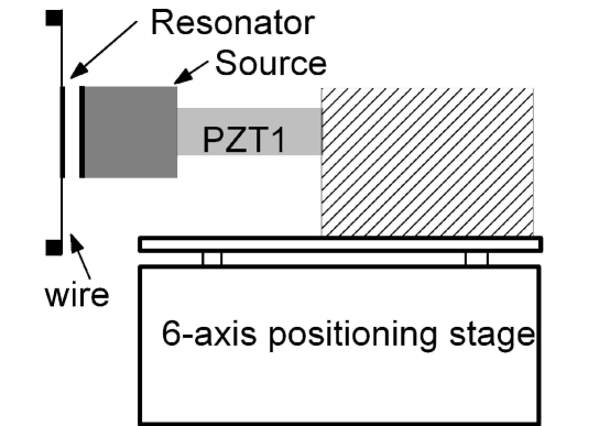
Figure 1: Side view showing the resonator, the source and the positioning system used for the parallelization.

The source, the resonator and the positioning stage are in a vacuum chamber, at a pressure of about 3 $\times$ 10^-6 mbar. The vacuum is provided by a vibration-free ion pump. The whole experiment lies inside a clean room (class 1000), with thermal stabilization at the level of $\Delta T$ = 0.1^∘, but showing a long term drift of the order of half a degree per day. The motion of the resonator is detected by means of a Michelson type interferometer set-up with a 1 mW amplitude stabilized He-Ne laser at 633 nm. The interference signal is collected by a photodiode, whose voltage readout $V_{M}$ converts into distance by using:

$$\delta x=\frac{\lambda}{2\pi}\frac{V_{M}}{V_{fr}}.$$ (3)

where $\lambda=633$ nm and $V_{fr}$ is the voltage corresponding to a interference fringe, in our case normally $V_{fr}=2.3$ V.

In order to achieve the maximum sensitivity of the resonator, particular care has been taken to minimize its free motion. The whole apparatus is mounted on a passive low frequency damper and on a floating optical table. As explained next, we want to minimize the low frequency noise, below a few Hz: the passive damper (Minus-k Technologies 250 BM 6) is a mechanical low pass filter with a cut-off frequency at 0.5 Hz in the transmissibility curve. The clean room also represents a quiet environment to avoid acoustical noise: all the electronics lie in a separate control room. Moreover, a special metallic enclosure has been constructed around the apparatus. This enclosure has walls equipped with copper tubes through which temperature stabilized water flows, thus allowing very good long term stability of the entire system and thus eliminating the temperature drifts of the clean room. We discovered that temperature stability is crucial in order to perform repeated measurements over several days. In our case a stability of 0.1 degree of the experimental apparatus has been obtained for a time span of several days.

2.2 Detection technique

The set-up presented in this paper is based on an amplitude homodyne detection technique, already described in [19].

A static detection scheme is not sensitive enough, because it is affected by low-frequency drifts due to thermal expansion, electronic instabilities, drift of the laser frequency. For this reason we use the dynamical homodyne detection technique: we move the source with a periodical movement in the direction of the resonator. The Casimir force acting between the two surfaces makes the resonator move, and its motion is detected using the interferometer. If the chosen frequency is well below the resonator proper frequency, a fixed phase difference will be present between source motion and resonator motion, thus allowing for vector averaging of the interferometer signal.

If between the source and the resonator there is a spatially dependent force $F(d)$, then the equation of motion of the equivalent harmonic oscillator is

$$m\ddot{x}_{r}(t)=-m{\omega}_{r}^{2}x_{r}(t)+F(d),$$ (4)

where $x_{r}(t)$ is the position of the resonator, $\omega_{r}=2\pi\nu_{r}$ is its angular proper frequency and $m$ its mass.

We can decompose the separation $d$ between source and resonator into two components, namely a fixed distance $d_{0}$ and a time-dependent component $x_{s}(t)$, due to the movement of the source, that is $d=d_{0}+x_{s}(t)$ ($|x_{s}/d_{0}|\ll 1$). The free motion of the resonator is considered much smaller and is neglected. In the case of a force of the form $F(d)=C/d^{n}$, a periodic modulation of the position of the source $x_{s}=x_{s}^{0}\cos\omega_{s}t$ (with $\omega_{s}\ll\omega_{r}$), results in (at first order):

$$F(t)=\frac{C}{d_{0}^{n}}\left(1-n\frac{x_{s}^{0}}{d_{0}}\cos\omega_{s}t\right).$$ (5)

The oscillation of the resonator will be at the same frequency, and its amplitude together with the value of the spring constant of the resonator allows a calculation of the force parameters. In the Fourier spectrum of the solution $x_{r}(t)$ of equation (4) there is a peak at the frequency $\nu_{s}=\omega_{s}/2\pi$, whose amplitude is:

$$A_{s}^{0}=n\frac{Cx_{s}^{0}}{m\omega_{r}^{2}d_{0}^{n+1}}.$$ (6)

An overall calibration of the system is obtainable using controllable electrostatic forces. In fact, a constant voltage $V$ between the resonator and the source will induce a force

$$F_{V}(d)=-\frac{1}{2}\epsilon_{0}S\left(\frac{V}{d}\right)^{2},$$ (7)

It is then possible to compare the amplitude induced by the Casimir force $A_{C}$ and the one obtained by the voltage calibration at fixed bias $A_{V}$:

$$A_{C} = \frac{1}{60}\frac{\pi^{2}\hbar cS}{m\omega_{r}^{2}d_{0}^{5}}x_{s}^{0}$$ (8)

$$A_{V} = \frac{\epsilon_{0}SV^{2}}{m\omega_{r}^{2}d_{0}^{3}}x_{s}^{0}.$$ (9)

The calibrations are useful to infer the parameters common to both expressions, without relying on their direct determination.

2.3 Stray effects

In order to measure the Casimir force, one must be able to eliminate or compensate other forces acting between the two plates. In particular, forces of electrostatic nature can be present. The origin of these forces can be divided into two different categories: residual bias voltage and patch potentials.

Even when two conductors are shortened together, a residual bias $V_{0}$ could be present between them due to contact potential. A counterbias $-V_{0}$ eliminates the effect of this residual potential, but one has to be sure that its value is not changing with time and gap separation. A careful study must be performed. Counterbias accuracy must be kept at a few mV level in order to disentangle the contribution of the Casimir force.

It is well known that local changes in the crystallographic directions exposed at the surface of a clean polycrystalline metal, as well as surface contaminations, give rise to a point-dependent surface density $m(\vec{x})$ of dipoles on the surface of a metal [20]. The presence of such an inhomogeneous double layer of charges results in a spatially varying electrostatic potential $V(\vec{x})$ at the metal surface, relative to its interior, known as ”patch” potential. This zero-mean electrostatic component cannot be eliminated by a counterbias, and gives rise to a force whose distance dependance is related to the spatial distribution of the patches. In order to calculate the force of attraction between the two plates, it is convenient to describe the patches with a characteristic length scale $\lambda_{L}$, which satisfies the condition:

$$d\ll\lambda_{L}\ll L$$ (10)

where $d$ is the gap separation between the plates having lateral dimension $L$. The patch potentials $V(\vec{x})$ can be split as:

$$V(\vec{x})=V^{(L)}(\vec{x})+V^{(S)}(\vec{x})$$ (11)

In this equation, $V^{(L)}(\vec{x})$ represents the long wavelength component, that does not vary appreciably under displacements smaller than $\lambda_{L}$ along the surface, while $V^{(S)}(\vec{x})$ represents the short wavelength component. Physically, $V^{(L)}(\vec{x})$ can be thought to arise from the charges of a few isolated impurities distributed over the surface of the plates, while $V^{(S)}(\vec{x})$ describes the patch potentials of the microscopic crystallites forming the surfaces. The corresponding variances $\sigma^{2}_{L}$ and $\sigma^{2}_{S}$ of the two components give rise to a force with a characteristic distance dependence. Following [20] it is possible to obtain a force of the form:

$$F(d)=\epsilon_{0}L^{2}\left(\frac{\sigma^{2}_{L}}{2d^{2}}+\frac{2\sigma^{2}_{S}}{k^{2}_{\rm max}-k^{2}_{\rm min}}\int^{k_{\rm max}}_{k_{\rm min}}dk\frac{k^{3}}{\sinh^{2}(kd)}\right)$$ (12)

where the wave numbers $k_{\rm max,min}=2\pi/\lambda_{\rm min,max}$ are related to the maximum and minimum sizes $\lambda_{\rm max,min}$ of the crystallites.

3 Experimental results

The homodyne detection technique has been optimized looking for the modulation frequency of the source position providing the best signal to noise ratio. Long noise spectra are taken at the beginning of each measurement session, as a result the source is normally modulated at frequencies between 7 Hz and 14 Hz. This frequency range, well below the resonator proper frequency, ensures a complete decoupling between source motion and resonator itself due to mechanical and electrical pick-ups, as it was checked by a very long run with the plates kept at a separation of about 50 microns. Most of the measurements have been performed with 45 nm amplitude for the source motion. The resonator motion noise was normally at the level of $3\cdot 10^{-11}$ m/$\sqrt{\rm Hz}$, but this figure was stable only at night, degrading by a factor of 2 during daytime.

By imposing an external bias voltage $V_{g}$ to the gap, it is then possible to calibrate the apparatus. This is done in order to obtain the value of the residual bias voltage $V_{0}$, the effective resonator mechanical response and the absolute gap width separation. Again, for a detailed description of these steps, we refer to a previous paper [18], while presenting here the most recent results.

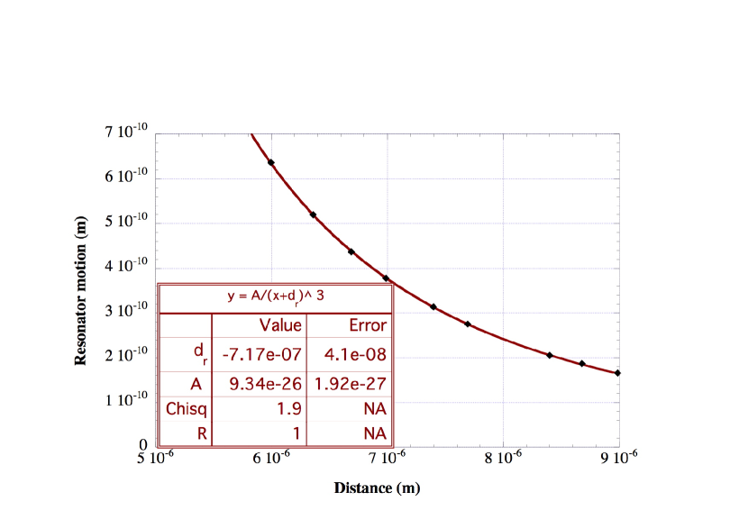
Figure 2: Measured signal versus distance when imposing an external bias voltage in the gap. The solid line is the best fist with a $1/d^{3}$ function. The experimental error for each measurement is smaller than the marker size.

By applying different values of an external bias voltage in the gap at fixed distance between the plates, one obtain the residual bias $V_{0}$. The resulting value was $V_{0}=244.7\pm 0.8$ mV, with a stability of 1-2 mV over a few days period. For longer time scales changes up to 10 mV have been observed: the reason for these changes is not yet clear to us, a possibility is the temperature of the apparatus. The value of $V_{0}$ has also been measured for different distances, and no change has been observed.

The measurement of the resonator motion versus gap separation, while keeping the external bias $V_{g}$ constant, provides the reference distance $d_{r}$ and also a cross check of the resonator mechanical response. The absolute gap separation is obtained by adding to the reference distance $d_{r}$ the displacement of the source given by the transducer PZT1.

Figure 2 shows a typical calibration response. The important parameter is the error on $d_{0}$, which is 40 nm. The coefficient $A$ differs from the expected one by about 5 %.

Casimir-type measurement are performed when $V_{g}=-V_{0}$, thus having a net zero voltage between the plates. Figure 3 shows the results obtained in 4 different measurement runs, performed in different days as indicated. The abscissa of the figure is the real gap separation already corrected using $d_{r}$. The ordinate shows the force derivative, i.e. the pulsating term of equation (5). Data are fitted with a function of the form $A/d^{n}$, where $A$ and $n$ are free parameters and $d$ is the gap separation. Results of the fits are rather astonishing: for $n$, values are in the range 3.5-5, and $A$ results to be way too large for being due to the Casimir force. Imposing a Casimir type dependence ($n=5$), the experimental coefficient $A$ is about 100 times larger than expected.

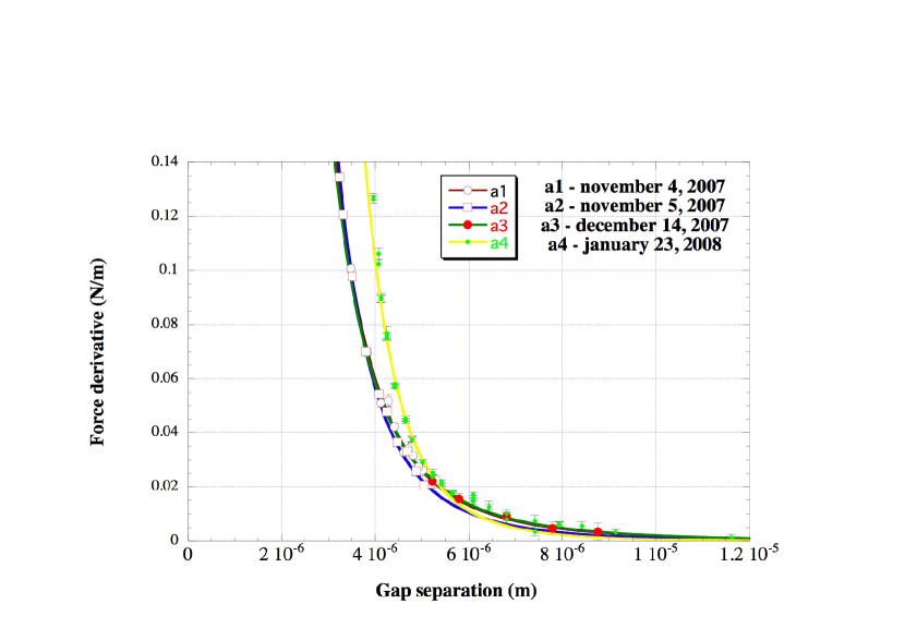
Figure 3: Summary of the measurements performed in the Casimir like configuration, i.e. a net zero voltage in the gap. Four different sets have been taken, corresponding to different measurement days. The abscissa is the absolute distance between the plates, as obtained by adding to the reference value $d_{r}$ the displacement of PZT1.

It is then important to try to understand the reasons for these results. The presence of an uncompensated bias voltage is excluded since a too large value would be necessary, much larger than the error on the determination of $V_{0}$. The influences of AC voltages on the gap have been eliminated by using filters along the connecting cables and replacing the cables themselves. Also the effect of the residual pressure was studied by changing the amount of gas in the chamber: no variation has been seen. A more detailed analysis concerns the presence of patch effects.

4 Patch effects

In order to study the presence of patches in the surface of the plates, a Kelvin probe analysis [21] has been done using plates similar to those mounted on the apparatus. Measurements of the work function across the samples were made by scanning the surfaces with a tip having an approximate diameter of 2 mm, with steps of 317.5 $\mu$m. The data (see Figure 4) showed that the work function exhibits significant fluctuations over distances of the order of one millimeter, and therefore this should be regarded as a long wavelength component of the patch potential in a force measurement involving separations of the order of a few microns. The variances of the work functions were found to be in the range 10 - 30 mV.

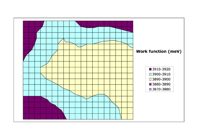
Figure 4: Kelvin probe analysis of a sample of bulk aluminium of the same type of the one used in the apparatus for measuring the Casimir effect. The measuring tip has a diameter of about 2 mm, each little square has a 0.35 mm side.

Another analysis that we performed was the X ray diffractometry, in order to determine the grain size of the microscopic crystallites forming the surfaces. This analysis gave a 0.1 $\mu$m size for the grains forming the aluminium bulk, and a 0.03 $\mu$m size for the aluminium coating on the silicon resonator. This analysis gives no information on the amplitude and variance of the work function associated with the crystallites, which should form the short wavelength component of the patch related force.

The three sets of data a1, a2, a3 of Figure 3 have been fitted together with the derivative $F^{\prime}(d)$, with respect to $d$, of the force $F(d)$ of equation (12), in order to extract from the fit the parameters related to the short and long wavelength components. The result is showed in Figure 5, the best fit is obtained with $\lambda_{\rm min}=3\,\mu$m, $\sigma_{S}=91.3$ mV, $\sigma_{L}=51.6$ mV. As it is clear from the figure, the fit is good, and the probable values for $\sigma_{S}$ and $\sigma_{L}$ appear both very reasonable. The favored value for $\sigma_{L}$ is perhaps a bit larger than what expected from the Kelvin probe measurement. However, it should be considered that the tip used is very thick (2 mm), and therefore their data actually represent smoothed measurements of the work function, over areas of 4 mm². The smoothing may have led to underestimate the real fluctuation of the work function at scales of, say, 200-300 microns.

On the other side, the value $\lambda_{\rm min}=3\,\mu$m is indicating that the short wavelength component is not the one seen by the X ray diffractometry. There could be some other patches, for example again due to impurities, with micron size areas, that it is not possible to see with an independent surface analysis. This leaves still some open question on the understanding of our data.

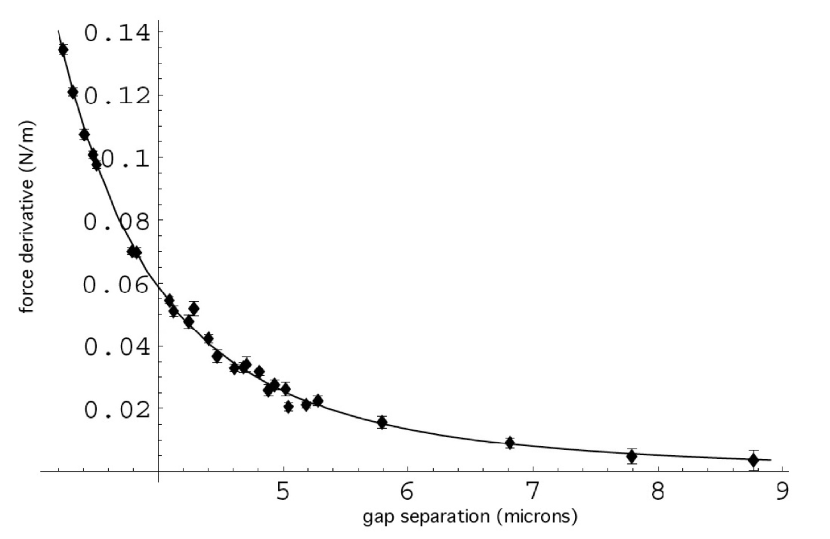
Figure 5: Fitting of the sets a1, a2, a3 of Figure 3. The solid line is the best fit with the derivative of the force (12), for $L=1$ cm, $\lambda_{\rm min}=3\,\mu$m, $\sigma_{S}=91.3$ mV, $\sigma_{L}=51.6$ mV.

5 Conclusions

We have set up an apparatus to measure the Casimir effect between parallel plates at separation in the range up to 5-6 microns. The possibility to achieve good parallelization and small gaps, down to 3 $\mu$m, using 1 cm² surfaces has been accomplished. The effort to measure the Casimir force is not yet successful, having encountered a much larger force of instrumental origin. Possible explanation of this force could be related to patch effects, but a clear identification of the patch potentials was not possible. It has to be noted that the use of aluminium might have enhanced the presence of patches: for this reason another set up is under construction with gold plated surfaces, which should reduce the effect of patches. If this problem will persist also using gold, this will put a serious obstacle in the measurement of the Casimir effect at a large separation.

Bibliography

Bibliography

- [1] Casimir, H. B. G. Proc. K. Ned. Akad. Wet. 51, 793 (1948).
- [2] Lifshitz, E. M. Sov. Phys. JETP 2, 73 (1956).
- [3] Bordag, M., Mohideen, U., and Mostepanenko, V. M. Phys. Rep. 353, 1 (2001).
- [4] Sparnaay, M. J. Physica (Utrecht) 24, 751 (1958).
- [5] van Blokland, P. H. G.M and Overbeek, J. T. G. J. Chem. Soc. Faraday Trans. I 74, 2637 (1978).
- [6] Lamoreaux, S. K. Phys. Rev. Lett. 78, 5 (1997).
- [7] Mohideen, U. and Roy, A. Phys. Rev. Lett. 81, 4549 (1998).
- [8] Decca, R. S., Fischbach, E., Klimchitskaya, G. L., Krause, D. E., López, D., and Mostepanenko, V. M. Phys. Rev. D 68, 116003 (2000).
- [9] Ederth, T. Phys. Rev. A 62, 062104 (2000).
- [10] Chan, H. B., Aksyuk, V. A., Kleiman, R. N., Bishop, D. J., and Capasso, F. Science 291, 1941 (2001).
- [11] Bressi, G., Carugno, G., Onofrio, R., and Ruoso, G. Phys. Rev. Lett. 88, 041804 (2002).
- [12] Genet, C., Lambrecht, A., and Reynaud, S. Phys. Rev. A 62, 012110 (2000).
- [13] Brown-Hayes, M., Dalvit, D. A. R., Mazzitelli, F. D., Kim, W. J., and Onofrio, R. Phys. Rev. A 72, 052102 (2005).
- [14] Hertzberg, M. P., Jaffe, R. L., Kadar, M., and Scardicchio, A. Phys. Rev. Lett. 95, 250402 (2005).
- [15] Obrecht, J. M., Wild, R. J., Antezza, M., Pitaevskii, L. P. , Stringari, S., and Cornell, E. A. Phys. Rev. Lett. 98, 063201 (2007) .
- [16] Casimir, H. B. G. , and Polder, D. Phys. Rev. 73, 360 (1948).
- [17] Antezza, M., Pitaevskii, L. P., Stringari, S., and Svetovoy, V. B. Phys. Rev. Lett. 97, 223203 (2006).
- [18] Antonini, P., Bressi, G., Carugno, G., Galeazzi, G., Messineo, G., and Ruoso, G., New J. Phys. 8, 239 (2006).
- [19] Bressi, G., Carugno, G., Galvani, A., Onofrio, R., Ruoso, G., and Veronese, F. Class. Quantum Grav. 18, 3943 (2001).
- [20] Speake, C.C., and Trenkel, C. Phys. Rev. Lett. 90, 160403 (2003).
- [21] Measurements were performed by KP Technology, Burn Street, Wick, Caithness, KW1 5EH, Scotland