Using the Memories of Multiscale Machines to Characterize Complex Systems

Abstract

A scheme is presented to extract detailed dynamical signatures from successive measurements of complex systems. Relative entropy based time series tools are used to quantify the gain in predictive power of increasing past knowledge. By lossy compression, data is represented by increasingly coarsened symbolic strings. Each compression resolution is modeled by a machine: a finite memory transition matrix. Applying the relative entropy tools to each machine’s memory exposes correlations within many timescales. Examples are given for cardiac arrhythmias and different heart conditions are distinguished.

Before understanding a complex system, one often needs to interpret the complex signals it generates. While it is easy to find correlations between arbitrarily separated pairs of points in a signal time series Voss , highly correlated signals can lack such pairwise correlations (Section I). Instead, at a higher resolution, one can estimate the joint probabilities of sequences of events and, eg., find the order of corresponding Markov chains Billingsley . Unfortunately the set of possible event sequences will generically increase exponentially with sequence length while becoming proportionately harder to estimate; i.e. what these methods gain in resolution over pairwise statistics, they lose in range. We must, however, expect Nature to show correlations which are both long-ranged and more than pairwise.

This Letter suggests a tool, akin to the autocorrelation, which is intuitive, sensitive to more than pairwise correlations and yet is long-ranged enough to capture the longtime correlations shown by some complex systems. It combines two core ideas: 1) a natural measure of the predictive power one gains as one has an increasingly long symbolic string (Sec. II-V); 2) use of lossy compression to express the dynamics of a complex system as a set of Markov sources (transition matrices) with each one representing the dynamics on a different timescale (VI-VIII). The following considers a system which, at any time $t$, can be in state $x_{t}$ chosen from an alphabet (finite set) $\mathcal{A}$. The system passes through states $x_{1},x_{2}...x_{T}$ at fixed intervals and the data is ergodic and stationary. From now on $x_{j},...x_{k}$ will be represented by $x^{k}_{j}$. Having addressed pairwise correlation measures in Section I, Sections II-VI develop a new means of mapping correlations in strings and VII-IX consider physiological examples and continuous time series.

I Pairwise Statistics Can Fail to Capture Structure. Any approach which investigates the time structure of a data string must be compared with conventional methods like the autocorrelation function. Pairwise measures, which compare a symbol at one point in a string with a (possibly different) symbol at another point, fail to capture conditional behavior on other intervening symbols. The following one-parameter, order-two transition matrix with alphabet $\mathcal{A}_{4}=\{A,B,C,D\}$ should remind the reader of this phenomenon; it can create strings without pairwise correlations. Using the notation that $X$ is a random variable and $x$ is a particular instantiation of that variable, it is of the form $p(X_{3}|X_{1}X_{2})$ with ($x_{i}\in\mathcal{A}_{4})$:

$$\mbox{\tiny{\emph{x}}}_{\mbox{\tiny{\emph{1}}}}{\mbox{\tiny{\emph{x}}}_{\mbox{\tiny{\emph{2}}}}\backslash^{{x}_{\it 3}}}$$

(1)

where $\Lambda^{\pm}=\frac{1}{4}\pm d$, the free parameter $d$ is $0\leq d\leq\frac{1}{4}$ and where $pq$ is any ordered pair, $p$ preceding $q$, other than $AA,BB,BA,AB$. One can prove that, for strings generated by this matrix, the probability of obtaining the symbol $u\in\mathcal{A}_{4}$ an interval $l\neq 0$ after $v\in\mathcal{A}_{4}$ is independent of both $l$ and $v$. The auto/cross correlations of such a series are thus indistinguishable from white noise (for explanations of symbolic autocorrelations see Voss Voss ). However, the string is highly structured; measures like ${\bf r}H_{n||m}$ below can expose this. Simple measures which reveal correlations between points, without having to create data objects which scale exponentially with order, can be very useful. The approach in Section VI yields data objects that both increase slowly with order/time and illuminate more than pairwise correlations.

II The Transition Entropy. If a string is sufficiently long, one can estimate transition probabilities $p(X_{t}|X_{t-m}^{t-1})$. It should be stressed that this paper is not, in the first instance, about the estimation of these probabilities; we will assume that they are given to us exactly Herzel94 . The following entropies investigate the structure of this order $m$ transition matrix.

Call $\small{H(X_{t})=\sum_{x_{t}\in\mathcal{A}}-p(x_{t})\log_{\tiny{2}}p(x_{t})}$ the Shannon entropy of $X_{t}$. The transition, or conditional, entropy ${\bf t}H_{m}$ is defined as follows:

$${\bf t}H_{m} = \sum_{x^{t-1}_{t-m}\in\mathcal{A}^{m}}p(x^{t-1}_{t-m})H(X_{t}|x^{t-1}_{t-m}),$$ (2)

This transition entropy, ${\bf t}H_{m}$, measures the entropy of predictions one makes when equipped with a length $m$ string, when one does not know what the string is. If each length $m$ string that occurs exactly predicts the next state, then ${\bf t}H_{m}=0$ (for the series $...ABABA...$ each length $1$ string uniquely determines its ensuing state: ${\bf t}H_{1}=0$). If no string imparts a predictive advantage then ${\bf t}H_{m}=H(X_{t})$ $\forall m$. Convexity arguments Berger show that ${\bf t}H_{m}\geq{\bf t}H_{n}$ ($n>m$).

III The Relative Transition Entropy. The relative transition entropy, ${\bf r}H_{n||m}$, defined below is a measure of gain in predictive power as one moves from knowledge of a length $m$ string to a length $n$ string ($n>m$). The relative entropy or Kullback-Leibler divergence Berger between the distribution $Q(X)$ and $P(X)$, where $X$ can take $|\mathcal{A}|$ different values, is: $D(Q||P)=\sum_{x\in\mathcal{A}}Q(x)\log\frac{Q(x)}{P(x)}$. It is often described as the average disbelief in a model’s predicted distribution $P$, when observing random outcomes $X$ from real data $Q$. By contrast, we will use it to capture the degree that predictions made when equipped with more knowledge of the past, represented by $Q$, are inconsistent with those made with reduced knowledge, $P$.

One can compare predictions about a symbol at time $t$ given knowledge of a particular set of preceding $n$ symbols ($x^{t-1}_{t-n}$) with predictions made when given only the preceding $m$ ($x^{t-1}_{t-m}$ with $n>m$). The divergence, $D(p(X_{t}|x^{t-1}_{t-n})||p(X_{t}|x^{t-1}_{t-m}))$, measures the information lost if one loses the knowledge that the sequence $x^{t-1}_{t-m}$ was preceded by $x^{t-m-1}_{t-n}$. Averaging over all strings $x^{t-1}_{t-n}$ yields the relative transition entropy ${\bf r}H_{n||m}$:

$${\bf r}H_{n||m}=\sum_{x^{t-1}_{t-n}}p(x^{t-1}_{t-n})D(p(X_{t}|x^{t-1}_{t-n})||p(X_{t}|x^{t-1}_{t-m})).$$ (3)

This quantifies the predictive power lost when one moves from having a length $n$ string of prior information to the shorter length $m$, for a randomly selected string $x^{t-1}_{t-n}$ Schreiber . Let us now establish a few properties of ${\bf r}H_{n||m}$. Using (2-3) one can readily prove that ${\bf r}H_{n||m}={\bf t}H_{m}-{\bf t}H_{n}$, $n>m$. If ${\bf t}H_{m}={\bf t}H_{n}$ then ${\bf r}H_{n||m}=0$. Since $D(Q||P)\geq 0$, with equality only when $Q=P$, we further know that if ${\bf r}H_{n||m}=0$ then $p(X_{t}|x^{t-1}_{t-n})=p(X_{t}|x^{t-1}_{t-m})$ $\forall X_{t},\;x^{t-1}_{t-n}$. The length $n$ and $m$ predictions are exactly the same. In general $D(Q||P)$ can be unbounded Berger , but here, some thought shows that $0\leq{\bf r}H_{n||m}\leq H(X_{t})$. We can now formulate a hierarchy of differential quantities. Defining the Shannon entropy for strings of length $n$ as $H_{n}=H(X^{t}_{t-n+1})$, one readily finds that ${\bf t}H_{n}=H_{n+1}-H_{n}$ and ${\bf r}H_{n||m}={\bf t}H_{m}-{\bf t}H_{n}$. Authors have noted that the way that $H_{n}$ and ${\bf t}H_{n}$ decrease with $n$, reveals structure in the string grassbergertending ; Bandt : in Section VI we will use ${\bf r}H_{n||m}$ to map these correlations Schreiber .

IV Example: ${\bf r}H_{n||m}$ for the distribution in Eq. 1. $p(X_{3}|X_{1}X_{2})$ yields the stationary state, $p(X_{1}X_{2})=\frac{1}{16}$ so $p(X_{2}|X_{1})=\frac{1}{4}$. By Eq. 3 one finds ${\bf r}H_{1||0}=0$ (comparing $p(X_{2}|X_{1})$ and $p(X_{2})$). Comparing $p(X_{3}|X_{1}X_{2})$ and $p(X_{3}|X_{2})$ shows that ${\bf r}H_{2||1}=\frac{1}{4}\log_{2}[2(\Lambda^{+})^{\Lambda^{+}}(\Lambda^{-})^{\Lambda^{-}}]$. I.e. knowing the current state is of no help in predicting the next state (${\bf r}H_{1||0}=0$) but knowing the current and preceding state does help (${\bf r}H_{2||1}>0$ and so ${\bf r}H_{2||0}>0$). Since, for $n>2,m>1$, ${\bf r}H_{n||m}=0$ one concludes that knowing more than the preceding and current state gives no further predictive advantage.

V Introducing a measure to detect concealed structure. We noted that if the predictions of length $m$ and $m+1$ strings differ then ${\bf r}H_{m+1||m}>0$; however, since Eq. 3 is an average, small changes in this quantity can hide dramatic changes between the structure of order $m+1$ and order $m$ transition matrices. One can readily construct examples where there exists a string $x^{t-1}_{t-m-1}$ such that $D(p(X_{t}|x^{t-1}_{t-m-1}||p(X_{t}|x^{t-1}_{t-m}))\gg{\bf r}H_{m+1||m}$. It is thus useful to introduce the quantity: $\small{\widehat{{\bf r}H}_{m+1||m}=\max_{x^{t-1}_{t-m}}D(p(X_{t}|x^{t-1}_{t-m-1}||p(X_{t}|x^{t-1}_{t-m})))}$ the maximum relative transition entropy over all strings $x^{t-1}_{t-m}$ in $A^{m}$. This measures when knowledge of a particular extra symbol imparts a large predictive advantage.

VI Introducing Multiscale Markov Sources. This section introduces a method for describing data from complex systems by fitting finite state machines with memories to each of their different time-scales. Consider coarsening time series to lower and lower time resolutions. For each resolution one might estimate a small, order $m$, transition matrix (Markov source is another name for transition matrix Berger ). Let us call these matrices, one for each resolution, a set of multiscale Markov sources. Suppose the real data was generated by a high order Markov source of order $l\gg m$. An order $l$ source (alphabet $\mathcal{A}$) has $|\mathcal{A}|^{l}(|\mathcal{A}|-1)$ parameters. By contrast, we will see that a corresponding set of multiscale Markov sources requires only $\sim\log l$ parameters. The sources thus form a compact multiscale representation of the data.

Let us now examine more details of the coarsening. We first break the symbolic series, $y^{T}_{1}$, $y_{i}\in\mathcal{A}$, into consecutive non-overlapping blocks, each $c^{r}$ symbols long. We fix $c$, the basic block size, and let $r$ vary to give different block sizes $c^{r}$ (increasing $r$ increases the block size and we will see that this lowers the resolution). Then we coarsen by mapping each possible block (of which there are $|\mathcal{A}|^{c^{r}}$) onto a single symbol from a smaller set $\mathcal{C}$ ($|\mathcal{C}|<|\mathcal{A}|^{c^{r}}$). The manner of this map will be discussed below. The new coarsened string at resolution $r$ has ${T/c^{r}}$ elements ${}^{r}x^{T/c^{r}}_{1}$ with ${}^{r}x_{i}\in\mathcal{C}$. From this string one can estimate an order $m$ Markov source, ${}^{r}_{m}M$. Supposing the raw data was generated by a source of order $l$, one might fix $|\mathcal{C}|$, $c$ and $m$ and vary $r$ to give a set of Markov sources ${}^{r}_{m}M$ with $r\in\{1,2,...\lceil\log_{c}\frac{l}{m}\rceil\}$. By choosing this range of $r$ values the set of sources has a similar memory to the order $l$ transition matrix. While the order $l$ source needs $|\mathcal{A}|^{l}(|\mathcal{A}|-1)$ parameters, the total number of parameters in the multiscale sources is $|\mathcal{C}|^{m}(|\mathcal{C}|-1)\lceil log_{c}\frac{l}{m}\rceil$. The set of Markov sources ${}^{r}_{m}M\;\forall r\leq\lceil\log_{c}\frac{l}{m}\rceil$ thus gives a compact multiscale dynamic model for the correlations at each timescale Dugatkin (see top diagram in Fig. 2).

Such lossy compression lies broadly within rate-distortion theory Berger . Distortion measures capture the lossiness of maps from blocks to single symbols. The following motivational example uses the crude Hamming distortion. Blocks of $c^{r}$ symbols, each symbol in $\mathcal{A}$, can be viewed as coming from an alphabet $\mathcal{B}_{c,r}$ of size $|\mathcal{A}|^{c^{r}}$. Call a compression a map $f:\mathcal{B}_{c,r}\rightarrow\mathcal{C}$. A map is optimal if a version reconstructed from the compressed string (using an inverse map $g:\mathcal{C}\rightarrow\mathcal{B}_{c,r}$) and the original string are as close as possible with respect to a given measure. The Hamming distortion is $d(g(f(X_{t})),X_{t})=\delta_{g(f(X_{t})),X_{t}}$ for $X_{t}\in\mathcal{B}_{c,r}$. Given $p(X_{t})$, the optimal map minimizes the expected symbol-by-symbol distortion between the reconstructed and original letters $<d(g(f(X_{t})),X_{t})>$. Here, some thought shows that the optimal $f$: (1) takes each of the $|\mathcal{C}|$ most probable symbols in $\mathcal{B}_{c,r}$ to a distinct symbol in $\mathcal{C}$ and (2) takes all other symbols to an arbitrary symbol in $\mathcal{C}$.

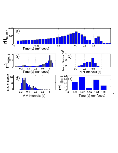
Figure 1: A patient with cardiac arrhythmia: a) The $m^{\rm{th}}$ bar gives the predictive advantage of knowing $m\tau$ seconds of past activity over knowing $m\tau-\tau$ seconds of activity (${\bf r}H_{m||m-1}$). $\tau=32$ms and $t\leq 35\tau$ (more than $99\%$ of all length $35\tau$ strings, picked uniformly at random from the data, occurred more than $300$ times). b) $\widehat{{\bf r}H}_{m||m-1}$ for the original data. c,d) The intervals between successive normal and ventricular beats respectively. e) ${\bf r}H_{m||m-1}$ for a coarsened string $r=1$, $c=12$, $|\mathcal{C}|=10$ each timestep is thus $\tau^{\prime}=0.384$s. For length 4 and 5 strings in the coarsened data, $97\%$ and $90\%$ respectively of all such strings picked uniformly at random occurred more than $300$ times.

VII Example: Sudden Cardiac Death. This section applies the above tools to heart arrhythmia. A simplified view of the heart is that, in any short interval, it can have a normal ($N$) or ventricular beat ($V$) or no beat at all ($\O$). The raw data is a list of times of beats labeled as $N$ or $V$ physionet . By discretizing time into blocks of $\tau=32$ms this list was converted into a symbolic string of the form ‘… $\O N\O V\O\O N$…’. The following uses 24 hours of heart data for a patient with many $V$ beats. Given this three-letter alphabet one can attempt to estimate a transition matrix of order $m$: $p(X_{t}|x^{t-1}_{t-m})\;\forall X_{t},x^{t-1}_{t-m}$ Courtemanche . Since $\tau\ll$ interbeat interval ($\sim 0.85$s) and the system is very structured, the size of the transition matrix grows slowly with $m$. Accommodation of finite size effects in the estimation of such transition matrices, is delicate Herzel94 and a crude approach was used here (partly justified by the wealth of data). The transition matrices can only give information about the data as a whole (rather than the behavior of the heart at any one time) as, alongside the presence of multiscale nonstationarities multiscale , this patient was particularly unhealthy. Fig. 1a) shows ${\bf r}H_{m||m-1}$ for the patient. As $m\tau$ (the duration of string one is given) increases towards the $N-N$ beat interval (see Fig. 1c)), one’s ability to make good predictions increases markedly. But, when $m\tau$ nears the heart beat interval, further knowledge gives less predictive advantage (because one is already equipped with knowledge of a characteristic time period of the process). As a result ${\bf r}H_{m||m-1}$ begins to fall around $0.7$s, mirroring the distribution in Fig. 1c). Beats with intervals $>1s$ are rare so ${\bf r}H_{m||m-1}$ for $m\tau>1$s is small. Fig 1b) plots $\widehat{{\bf r}H}_{m||m-1}$ (with the strong promise that all strings considered occurred more that $300$ times in the data). It reveals hidden structure between $0.2$ and $0.4$s. This peak is the compound effect of short $V-V$ events and misannotations in the uncorrected record (see Fig. 1d)). The coarsened data, Fig. 1e), reveals structure on another timescale: one sees that a large part of the predictive knowledge is contained in the first second of activity but another characteristic timescale, open to physiological interpretation, appears in the range $1.19-1.54$s. Plots like Fig. 1 might distinguish between heart conditions, since these can depend on dynamics of a few seconds Schulte .

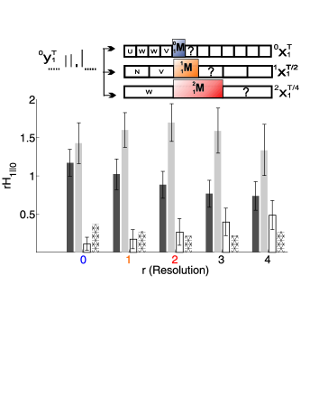
Figure 2: Above: schematic of vector quantization (${}^{0}y^{T}_{1}\rightarrow{}^{r}x^{{T}/{c^{r}}}_{1}$) and multiscale Markov sources ${}^{r}_{1}M$. Main: The black, grey and white bars are the means, $\pm$ standard errors, of groups of patients who were healthy, experiencing congestive heart failure and atrial fibrillation respectively. Unphysiological and ectopic beat intervals were filtered (as in Costa ) and hourly trends removed. The fourth, hatched, columns are for random phased $1/f$ noise. The $x$ axis considers the beat interval data at five different resolutions $r=0...4$ $c=2$. At each resolution $rH_{1||0}$ is found; this measures the extra predictive power from knowing one symbol over knowing none. Gaussian white noise has $rH_{1||0}\rightarrow 0\;\forall r$ and is not plotted (Brownian noise has $rH_{2||1}\rightarrow 0\;\forall r$) .

VIII Continuous time series. Multiscale Markov sources can also be found for continuous time series (eg. wind speed) as well as symbolic strings. The data, sampled at $T$ times, is again broken up into blocks of $c^{r}$ consecutive points and coarsened. The alphabet we compress to is now a set of $|\mathcal{C}|$ letters with each one representing a different motif of $c^{r}$ consecutive reals. We allocate each block of raw data to its closest motif using a mean-square distance. For example, suppose we want to compress blocks of two data points $(c=2,r=1)$ to one of three symbols and we are given a three letter code book with three motifs: $\mathcal{C}=\{N=(1,1),\,V=(0.1,2),\,U=(10,10)\}$. Using the mean-square distance, the sequence of continuous data ${}^{0}y^{T}_{1}=...|1\;1.1|0.2\;1.5|1.1\;1.01|...$ is optimally represented by ${}^{1}x^{{T}/{2}}_{1}=...|N|V|N|...$ See Fig 2. The optimal set of motifs, for a fixed $|\mathcal{C}|$, allow the compressed sequence to reconstruct the original with minimum total mean-square error costacomm . A selection of algorithms exists for finding optimal motifs (vector quantizers Berger ). In our case, such algorithms have as input the set of $T/c^{r}$ blocks of length $c^{r}$ and the value of $|\mathcal{C}|$. They output the set, $\mathcal{C}$, of motifs of length $c^{r}$ which minimizes the total mean-square error for this block size. Given these motifs one can then convert the continuous time series into its closest symbolic equivalent (see the above example: ${}^{0}y^{T}_{1}$ $\rightarrow{}^{1}x^{{T/2}}_{1}$ see Fig. 2). Given this string of symbols generated from blocks of $c^{r}$ real valued data points, one again determines ${}^{r}_{m}M\;\forall r$.

IX Example. Fig. 2 applies this idea to three different groups of cardiac patients physionet , using the Generalized Lloyd algorithm to find the appropriate set of motifs, $\mathcal{C}$, for each resolution, $r$ Berger . The raw cardiac data was an ‘interval series’: each data point being the time interval between successive heart beats. The matrix ${}^{r}_{1}M$ was found for $r=0...4$, $c=2$, $|\mathcal{C}|=10$ and the extra predictive power from knowing one symbol was estimated: $rH_{1||0}$. The three different heart conditions can be distinguished (for comparable results see Costa ); healthy hearts show a slow loss in predictability, the disordered beats that occur in atrial fibrillation yield a low degree of predictability whereas congestive heart failure shows an increase in predictability at some scales.

X Conclusion. This paper presented a means of producing a one parameter map of predictive knowledge acquired as one is equipped with increasingly long substrings of a symbolic data set. It suggests that lossy compression allows this short range mapping technique to be compactly extended to the study of longer ranged correlations. Examples are given where different heart conditions are distinguished and characterized using these methods. Underlying this work is the view that dynamical signatures of some systems can be found by treating them as sets of Markov sources with each source characterizing dynamics on a different timescale.

Thanks to M Costa, A Goldberger, C-F Lee and C-K Peng

References

- (1) Symbolic Examples: Fourier: R.F. Voss, Phys. Rev. Lett. 68, 3805 (1992); Walsh-Fourier etc.: D. Stoffer, J. Amer. Statist. Assoc. 86, 461 (1991); D. Stoffer et al. Biometrika 180, 611 (1993); Mutual information: A. M. Fraser and H. L. Swinney, Phys. Rev. A 33, 1134 (1986).
- (2) From three fields: P. Billingsley, Ann. Math. Stat. 32, 12 (1961); N. Merhav et al IEEE Trans. Inf. Theory 35, 1014 (1989); M.J. van der Heyden et al Physica D 117, 299 (1997).
- (3) H. Herzel , Chaos, Solit. Fract. 4, 97 (1994).
- (4) T. Cover J. Thomas, Elements of Information Theory (J. Wiley and Sons, NY, 1991); T. Berger, Rate Distortion Theory (Prentice-Hall, Englewood Cliffs, NJ, 1971); A. Gersho and R. Gray, Vector Quantization and Signal Compression (Kluwer Academic, Boston, MA 1992).
- (5) T. Schreiber, Phys. Rev. Lett. 85, 461 (2000) introduces the ‘transfer entropy’ to reveal causal links between two time series. reveals causal connection in the same series, and can be seen as the self transfer entropy.
- (6) P. Grassberger, Int. J. Theor. Phys 25, 907 (1986); W. Ebeling and G. Nicolis, Europhys. Lett. 14, 191 (1991).
- (7) Ch. Bandt and B. Pompe, J. Stat. Phys. 70, 967 (1993).
- (8) This can be connected with multiresolution source coding: eg. D. Dugatkin (2004) Caltech E. Eng. Thesis.
- (9) Databases: www.physionet.org. Fig. 1 Sudden Cardiac Death Holter Fig. 2 the entire MIT-BIH Normal Sinus Rhythm and BIDMC Congestive Heart Failure; Fibrillation Data from Costa .
- (10) M. Courtemanche , Am. J. Physiol. 257, H693 (1989) extracts transition matrices from arrhythmias but discards interbeat intervals. Many papers have applied symbolic dynamics to hearts but, to my knowledge, exclude beats and tend to record the change in beat intervals symbolically eg. J. Kurths , Chaos 5, 88 (1995).
- (11) P. Bernaola-Galvan , Phys. Rev. Lett. 87, 168105 (2001).
- (12) V. Schulte-Frohlinde , Phys. Rev. E 66, 031901 (2002).
- (13) A generalization of the coarsening in Costa et al Costa .
- (14) M. Costa et al, Phys. Rev. Lett. 89, 68102 (2002).