Catastrophic Photo-z Errors and the Dark Energy Parameter Estimates with Cosmic Shear

Abstract

We study the impact of catastrophic errors occurring in the photometric redshifts of galaxies on cosmological parameter estimates with cosmic shear tomography. We consider a fiducial survey with 9-filter set and perform photo-z measurement simulations. It is found that a fraction of $1\%$ galaxies at $z_{\rm spec}\sim 0.4$ is misidentified to be at $z_{\rm phot}\sim 3.5$. We then employ both $\chi^{2}$ fitting method and the extension of Fisher matrix formalism to evaluate the bias on the equation of state parameters of dark energy, $w_{0}$ and $w_{a}$, induced by those catastrophic outliers. By comparing the results from both methods, we verify that the estimation of $w_{0}$ and $w_{a}$ from the fiducial 5-bin tomographic analyses can be significantly biased. To minimize the impact of this bias, two strategies can be followed: (A) the cosmic shear analysis is restricted to $0.5<z<2.5$ where catastrophic redshift errors are expected to be insignificant; (B) a spectroscopic survey is conducted for galaxies with $3<z_{\rm phot}<4$. We find that the number of spectroscopic redshifts needed scales as $N_{\rm spec}\propto f_{\rm cata}\times A$ where $f_{\rm cata}=1\%$ is the fraction of catastrophic redshift errors (assuming a 9-filter photometric survey) and A is the survey area. For $A=1000\hbox{ deg}^{2}$, we find that $N_{\rm spec}>320$ and 860 respectively in order to reduce the joint bias in $(w_{0},w_{a})$ to be smaller than $2\sigma$ and $1\sigma$. This spectroscopic survey (option B) will improve the Figure of Merit of option A by a factor $\times 1.5$ thus making such a survey strongly desirable.

1 Introduction

The weak gravitational lensing effect by large scale structures, namely the cosmic shear, is believed to be a powerful tool to measure the cosmological parameters including the equation of state of dark energy. Over the last ten years, weak lensing observations have already provided increasingly better constraints on the matter density $\Omega_{M}$ and the amplitude of mass fluctuations often represented by $\sigma_{8}$, the $rms$ amplitude of the smoothed and linearly extrapolated mass density perturbations on the scale of $8\hbox{ Mpc}\ h^{-1}$ (Hoekstra, Yee & Gladders 2002, Jarvis et al. 2003, Rhodes et al. 2004, Heymans et al. 2004, Hoekstra et al. 2006, Semboloni et al. 2006, Massey et al. 2007, Benjamin et al. 2007, Fu et al. 2008). Their contributions to the constraints on the total neutrino mass have also been investigated (Tereno et al. 2008, Gong et al. 2008, Ichiki et al. 2008, Li et al. 2008). Several more ambitious weak lensing surveys targeting at hundred to thousand times larger areas, such as DES, LSST, JDEM and EUCLID, are being planned aiming at exploring the properties of dark energy in great detail.

Future large surveys are expected to be able to control statistical errors to insignificant levels. Therefore different systematics can become dominant sources of contaminations in future weak lensing studies, and should be investigated carefully. These include the effect of the point spread function (PSF) (e.g., Amara & Refregier 2008), the methodology in the shear measurement (Bacon et al. 2001, Erben et al. 2001, Hirata & Seljak 2003, Heymans et al. 2006, Massey et al. 2007, Miller et al. 2007, Kitching et al. 2008, Bridle et al. 2008, Ngan et al. 2008, Semboloni et al. 2008), redshift errors (Ma et al. 2006, Huterer et al. 2006), intrinsic alignments of source galaxies (see Heavens 2001 for a review, Bridle & King 2007, Fan 2007), uncertainties in the computation of the non-linear power spectrum (see discussion in Huterer 2002, Van Waerbeke et al. 2002), and so on. In this paper, we focus on the impact of the photometric redshift errors on cosmological studies.

The necessity of measuring vast amount of galaxy redshifts in cosmic shear observations makes the multi-color photometric determination of redshifts the only feasible way in obtaining the redshift information of source galaxies. However the inaccuracy of photometric redshifts can contaminate considerably the cosmological information embedded in cosmic shears (Huterer et al. 2006; Ma et al. 2006; Amara & Refregier 2007; Wittman et al. 2007; Abdalla et al. 2008; Margoniner & Wittman 2008; Stabenau et al. 2008). Taking into account the bias and the scatter of $z_{\rm phot}$ with respect to $z_{\rm spec}$, Ma, Hu & Huterer (2006) analyze the corresponding degradation of the constraints on dark energy. It is found that these errors can completely erase the additional information from tomographic lensing observations. In order to make full use of the advantage of the tomographic binning, both the bias and scatter of $z_{\rm phot}$ have to be known to better than 0.003-0.01. Amara & Refregier (2007) and Abdalla et al. (2008) pay special attention to the so-called catastrophic errors in $z_{\rm phot}$, the outliers with $|z_{\rm spec}-z_{\rm phot}|>1$, and explore their effects on the figure of merit of dark energy parameter constraints.

While most of the existing studies concentrate on the error range of parameter constraints, the systematic bias in the determination of cosmological parameters due to the photometric redshift errors should also be carefully analyzed. A large systematic bias can lead to a completely wrong conclusion on the values of the cosmological parameters although the statistical errors may be small (Amara & Refregier 2008). Our study presented in this paper emphasizes precisely this aspect of effects on dark energy parameter estimates arising from catastrophic failures in photo-z measurements. We focus on a survey with similar design as described in Aldering et al. (2004), with its 9-filter set described also in Dahlen et al. (2008) and Jouvel et al. (2009 in prep.). We analyze in particular the bias on dark energy parameter estimates induced by the catastrophic failures occurred around $(z_{\rm spec},z_{\rm phot})\sim(0.4,3.5)$. And we investigate in detail the requirements of the number of spectroscopic redshift measurements to retrieve the correct estimates.

The outline of the paper is as follows. In §2, we introduce the methods to describe the lensing observables and to evaluate the biases. We present the results of bias in §3. In §4, we discuss the calibration requirements to remove the biases due to the catastrophic failures. Discussions and conclusions are given in §5.

2 Methodology

In this section, we describe the formalism of lensing observables. Based on simulation results, we then model the source galaxy distribution with catastrophic failures taken into account. Finally we discuss the methods to evaluate the corresponding biases on dark energy parameter estimates, without and with spectroscopic calibration.

2.1 Lensing Observables

The convergence power spectrum $P_{ij}^{\kappa}(\ell)$ for the $i$th and $j$th redshift bin can be expressed as (see Kaiser 1992, Kaiser 1998, Ma et al. 2006)

$$P_{ij}^{\kappa}(\ell)=\int_{0}^{\infty}dz\,{W_{i}(z)\,W_{j}(z)}{H(z)\over D^{2}(z)}\,P\!\left(k_{\ell},z\right),$$ (1)

where $H(z)$ is the Hubble parameter and $D(z)$ is the comoving angular diameter distance. The matter power spectrum $P(k_{\ell},z)$ with $k_{\ell}=\ell/D(z)$ is computed from the linear transfer function of Bardeen et al. (1986), and then the non-linear fitting function of Peacock & Dodds (1996). The weighting function $W_{i}$ is given by

$$W_{i}(z) = {3\over 2}\,\Omega_{m}\,{H_{0}^{2}D(z)\over H(z)}(1+z)$$ (2)

$$\times\int_{z}^{\infty}dz^{\prime}{n_{i}(z^{\prime})}{D_{LS}(z,z^{\prime})\over D(z^{\prime})}\,,$$

where $D_{LS}(z,z^{\prime})$ is the angular diameter distance between $z$ and $z^{\prime}$, and $n_{i}$ is the galaxy distribution (normalized to unity) of the $i$th redshift bin. We employ the overall galaxy distribution of the form (Smail et al. 1994)

$$n(z)\propto z^{\alpha}\exp\left[-(1.41z/z_{\rm med})^{\beta}\right]$$ (3)

where $z_{\rm med}$ is the median redshift of a survey and we take $\alpha=2,\ \beta=1.5$.

Considering only the shot noise and the Gaussian sample variance, the covariance matrix of the lensing observables can be written as (e.g., Huterer et al. 2006, Ma et al. 2006)

$${\rm Cov}\left[C^{\kappa}_{ij}(\ell^{\prime}),C^{\kappa}_{kl}(\ell)\right]={\delta_{\ell\ell^{\prime}}\over(2\ell+1)\,f_{\rm sky}\,\Delta\ell}\,\left[C^{\kappa}_{ik}(\ell)C^{\kappa}_{jl}(\ell)+C^{\kappa}_{il}(\ell)C^{\kappa}_{jk}(\ell)\right].$$ (4)

where $\Delta\ell$ is the band width in multipole $\ell$, and $f_{\rm sky}$ is the fractional sky coverage of a survey. The total power spectrum $C^{\kappa}_{ij}$ is given by

$$C^{\kappa}_{ij}=P_{ij}^{\kappa}+\delta_{ij}{\sigma_{\gamma}^{2}\over{n}_{g}^{i}}\,,$$ (5)

where $\sigma_{\gamma}^{2}$ is the variance of each component of the intrinsic ellipticity of source galaxies, and $n_{g}^{i}$ is the surface number density of galaxies in the $i$th bin.

In our study, we consider a fiducial space-based survey with $f_{\rm sky}=0.025$, corresponding to 1000 $\hbox{deg}^{2}$, the summation of $n_{g}^{i}$, i.e., the total surface number density of source galaxies $n_{g}^{\rm tot}$, is taken to be $100$ arcmin^-2, $\sigma_{\gamma}$=0.22 and $z_{\rm med}$=1.26. We are aware of the likely extension of the survey area. Thus in analyzing the requirement of the spectroscopic redshift calibration, we derive a scaling relation that allows us to estimate the corresponding calibration requirement for any survey area and any catastrophic error fraction.

Investigations by Ma et al. (2006) show that tomographic analyses with multi-bins of source galaxies (denoted as $N_{\rm bin}$) can improve the statistical errors on cosmological parameter constraints considerably in comparison with those of 2-D analyses. The improvement increases with the increase of $N_{\rm bin}$. On the other hand, we cannot gain much further improvement with $N_{\rm bin}>5$. Hence throughout the paper, we consider lensing tomography with $5$ equally spaced redshift bins within the range of $z=[0,\ 3]$. All galaxies with $z>3$ are simply added to the last bin. The resulting redshift binning is illustrated in Figure 2.

2.2 Modeling galaxy distribution with catastrophic failures

Photometric estimations of galaxy redshifts through multi-waveband observations largely depend on the characteristic features of the spectral energy distribution (SED) of galaxies, such as the Lyman break and Balmer/$4000\AA$ break. The locations of the features give us the redshift information of the galaxies. Therefore the accuracy of photometric redshifts is sensitive to the wavelength coverage of observations. It is also affected by the observational signal-to-noise ratio and the estimation method. Besides, the spectroscopic calibration plays an important role in improving the accuracy of photo-z, which shall be discussed specifically in §4.

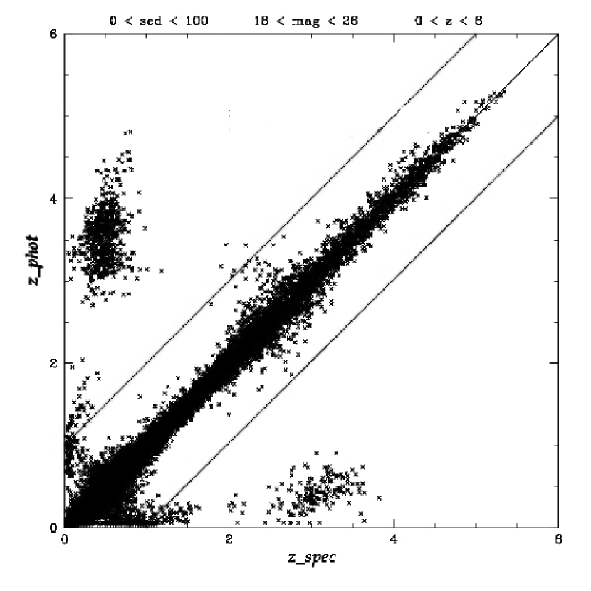
Figure 1: Result of LePhare simulation for our fiducial survey with a 9-filter set. A magnitude cut of 26 AB is set to fit the median redshift of the survey. The $2$ grey lines show the borders inside which the relation $|z_{\rm spec}-z_{\rm phot}|<1$ holds.

To realistically assess the accuracy of photometric redshifts for our survey, we first consider a 9-filter set which covers a wavelength range from visible blue to infrared with $\lambda\sim 390\hbox{ nm}$ to $\sim 1700\hbox{ nm}$ (For specific definition, see Dahlen et al. 2008). Then a series of simulations are carried out . The details of the simulations will be presented in Jouvel et al. (2009 in prep.). Here we give a brief description. The simulations are performed with the ’Le Phare’ software. First we generate galaxies according to the GOODS luminosity function by Dahlen et al. (2005), each with an assigned spectrum based on the Coleman Extended templates (Coleman et al. 1980). This set of templates contains $66$ spectra obtained by interpolating between $5$ standard spectra: elliptical, Sbc, Scd, irregular and star forming galaxies. We then apply the filtering process to the simulated spectra with the 9-filter set. We thus obtain the SED for each simulated galaxy. The magnitudes of galaxies are randomly assigned in accordance with the properties of our fiducial survey. The photometric redshift for each galaxy is then computed using the LePhare photometric redshift code. The results are shown in Figure 1.

It is seen that scatters and biases around $z_{\rm spec}$ exist for $z_{\rm phot}$. Besides, there are notable islands in the $z_{\rm spec}$-$z_{\rm phot}$ plot. The dominant one is located at $z_{\rm spec}\sim 0.4$ and $z_{\rm phot}\sim 3.5$, which accounts for more than $50\%$ of the galaxies with $|z_{\rm phot}-z_{\rm spec}|>1$. This island obviously comes from the confusion of the $4000\AA$ break with the Lyman break in galaxy SEDs due to the limited wavelength coverage. It is found that the fraction of galaxies with such large catastrophic errors is about $1\%$ of the total number of galaxies. In our study, we particularly analyze the effect of this island on the constraints of dark energy parameters.

To characterize the true distribution of galaxies whose photometric redshifts suffer from catastrophic failures, we use the following Gaussian distribution with the form

$$A_{\rm cata}\exp\bigg{[}-{(z-z_{m})^{2}\over 2\sigma^{2}}\bigg{]},$$ (6)

where the ’true’ mean redshift of the island $z_{m}=0.398$ and the standard deviation $\sigma=0.108$ are obtained from fitting to the spectral(true)-z distribution histogram of the island. The parameter $A_{\rm cata}$ is determined by normalizing the Gaussian distribution to the overall fraction of catastrophic failures $f_{\rm cata}=0.01$. Then in a tomographic division according to galaxies’ photometric redshifts, this part will be mistakenly shifted from low-z bin to another high-z bin. Specifically, for the $N_{\rm bin}=5$ tomography we consider, the $1\%$ galaxies with their true-z falling in the first bin are assigned to the last (5th) bin whose redshift range is $z_{\rm phot}>2.4$.

2.3 Evaluation of biases on dark energy parameter estimates

Once the distribution of catastrophic failure fraction is known, we can evaluate the biases it induces on dark energy parameter estimates.

As mentioned in the previous subsection, we need to be aware of the fact that observationally, source galaxies are assigned to different redshift bins in terms of their ’observed’ photometric redshifts rather than their true redshifts. Hence, a fraction of low redshift galaxies can be mistakenly distributed to high-redshift bins due to the catastrophic errors. As a consequence, weak lensing signals from those relevant tomographic bins are perturbed and biases on cosmological parameter estimates may arise, if models used to fit the data were not modified correspondingly.

Concerning the fiducial survey in this study, we know from simulations that there will be $f_{\rm cata}=0.01$ galaxies being misplaced into the 5th bin (denoted as ’Bin-5’), whilst their true redshifts are within the range of the first bin (denoted as ’Bin-1’). The true distribution of this catastrophic failure part can be described with Eq. (6) and will be labeled as Bin-cata for convenience in the following discussion. Note that the true z-range of Bin-cata is within the z-range of Bin-1.

For Bin-1, when Bin-cata galaxies within it are misplaced in Bin-5 due to catastrophic redshift errors, the number of galaxies contained in Bin-1 is reduced. The redshift distribution of the galaxies left in it also changes somewhat in comparison with the true distribution without the catastrophic errors. The number change in Bin-1 does not affect the lensing signal because the galaxy distribution within the bin is always normalized to unity. The shape change of the redshift distribution in the bin may have some effects. On the other hand, however, this change may already be included in the modeled overall redshift distribution of galaxies derived from photometric redshifts. Thus in our consideration, we assume that the misplacement of Bin-cata does not affect the lensing signal from Bin-1.

For bins in between Bin-1 and Bin-5, obviously the lensing signals should be kept unperturbed. Combining the previous analysis for Bin-1, we thus get $\bar{C}_{ij}^{\kappa}(\ell)=C_{ij}^{\kappa}(\ell)$, where $\rm i,j=1,...,4$.

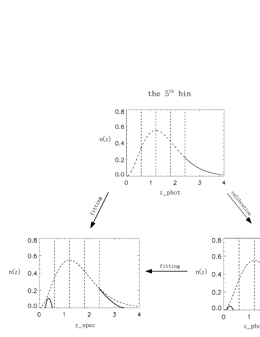
Figure 3: A sketch to explain where the bias comes from in cases without and with calibration. The top panel shows the ’observed’ photo-z distribution of Bin-5. Bottom-left: the true (spectral) distribution of Bin-5. Bottom-right: an example of the calibrated distribution of Bin-5, derived from an individual realization of calibration simulations.

To the contrary, the lensing signals from Bin-5 get perturbed. As shown in the bottom-left panel of Figure 3, it in fact consists of two parts of galaxies, one with their true redshifts falling in Bin-5 and the other being a contamination from Bin-cata. Correspondingly, besides the auto spectra of Bin-5, those cross spectra with one of the bins being Bin-5 will also be affected. In this case, those convergence power spectra can be expressed as

$$P_{i5}^{\kappa}(\ell)=\int_{0}^{\infty}dz\,{W_{i}(z)\,W_{5}(z)}{H(z)\over D^{2}(z)}\,P\!\left(k_{\ell},z\right),\ \ \ \ \ (\rm i=1,...,5)$$ (7)

with

$$W_{5}(z)=\cdot\cdot\cdot\,\int_{z}^{\infty}dz^{\prime}{n_{5}(z^{\prime},f_{\rm cata},z_{m},\sigma)}{D_{LS}(z,z^{\prime})\over D(z^{\prime})}\,$$ (8)

where we omit the antecedent terms identical to those in Eq. (2). The true (spectral) galaxy distribution of Bin-5 can be written as

$$n_{5}(z,f_{\rm cata},z_{m},\sigma) = {1\over f_{5}+f_{\rm cata}}\,\left[n_{5}(z)+n_{\rm cata}(z,f_{\rm cata},z_{m},\sigma)\right]$$ (9)

$$= {1\over f_{5}+f_{\rm cata}}\,\{n_{5}(z)+A_{\rm cata}\exp\bigg{[}-{(z-z_{m})^{2}\over 2\sigma^{2}}\bigg{]}\}$$

where $1/(f_{5}+f_{\rm cata})$ is to normalize $n_{5}(z,f_{\rm cata},z_{m},\sigma)$ to be unity, with $f_{5}$ being the overall fraction of galaxies with their true redshifts falling in Bin-5. Here the right side terms $n_{5}(z)$ and $n_{\rm cata}$ are normalized to their overall fraction $f_{5}$ and $f_{\rm cata}$, respectively. $A_{\rm cata}$ is thus determined by $f_{\rm cata}$, as mentioned in the paragraph following Eq. (6). With the substitution $n_{g}^{5}\rightarrow n_{g}^{5}+n_{g}^{\rm cata}$ in Eq. (5), finally we get the ’observed’ total spectra $C_{i5}^{\kappa}(\ell,f_{\rm cata},z_{m},\sigma)$, where $f_{\rm cata}=0.01,z_{m}=0.398,\sigma=0.108$ and $i=1,...,5$.

In practical analysis, when calculating the ‘theoretically expected’ lensing signals for Bin-5, we have no knowledge, in the case without spectroscopic calibration, of the fraction of low redshift galaxies and regard all the galaxies being at high redshifts; or in the case with inadequate spectroscopic calibration, we have inaccurate knowledge therefore can make unprecise estimation of the fraction and distribution of low-z galaxies (see Figure 3). The former can be denoted as $\bar{C}_{i5}^{\kappa}(\ell,0,c,c)$, with c being an arbitrary constant. The latter case gives $\bar{C}_{i5}^{\kappa}(\ell,\bar{f}_{\rm cata},\bar{z}_{m},\bar{\sigma})$, where the estimations $\bar{f}_{\rm cata},\bar{z}_{m}$ and $\bar{\sigma}$ can deviate from their true values depending on the calibration size.

Consequently systematic biases may arise when the theoretically expected signals $\bar{C}_{ij}^{\kappa}$ are compared with the observed ones $C_{ij}^{\kappa}$ to constrain cosmological parameters. As an approximation, a simple extension of the Fisher matrix formalism can be used to compute the bias in cosmological parameters with (see Huterer et al. 2006, Amara & Refregier 2008)

$$\delta p_{i}=F_{ij}^{-1}\,\sum_{\ell,\alpha,\beta}\left[C_{\alpha}^{\kappa}(\ell)-\bar{C}_{\alpha}^{\kappa}(\ell)\right]{\rm Cov}^{-1}\left[C_{\alpha}^{\kappa}(\ell),C_{\beta}^{\kappa}(\ell)\right]\,{\partial\bar{C}_{\beta}^{\kappa}(\ell)\over\partial p_{j}}$$ (10)

where $\alpha$ and $\beta$ each denote a pair of redshift bins. The term $\left[C_{\alpha}^{\kappa}(\ell)-\bar{C}_{\alpha}^{\kappa}(\ell)\right]$ reflects the bias on the shear signals. The covariance of the cross power spectra is given in Eq. (4). $F_{ij}^{-1}$ is the inverse of the Fisher matrix

$$F_{ij}=\sum_{\ell}\,\left({\partial{C}\over\partial p_{i}}\right)^{T}\,{\rm Cov}^{-1}\,{\partial{C}\over\partial p_{j}},$$ (11)

where ${C}$ is the column matrix of the convergence power spectra and ${\rm Cov}^{-1}$ is the inverse of the covariance matrix.

Eq. (10) is a linear approximation around the fiducial model. On the other hand, the true extent of bias can be quantified by a direct chi-square fitting method, by minimizing

$$\chi^{2}=\sum_{\ell,\alpha,\beta}\left[C_{\alpha}^{\kappa}(\ell)-\bar{C}_{\alpha}^{\kappa}(\ell)\right]{\rm Cov}^{-1}\left[C_{\alpha}^{\kappa}(\ell),C_{\beta}^{\kappa}(\ell)\right]\,{\left[C_{\beta}^{\kappa}(\ell)-\bar{C}_{\beta}^{\kappa}(\ell)\right]}.$$ (12)

In our analyses, we will utilize both bias evaluation methods. The comparison of their results permits us to quantify the extent to which the linear approximation is valid. We shall come back to this in the following section, associated with the specific study for our fiducial survey.

Throughout our study, a 7 parameter fiducial flat cosmological model is assumed. For equation of state of dark energy, we consider the form $w(z)=w_{0}+{w_{a}}z/(1+z)$ (Chevallier & Polarski 2001). The fiducial values of the 7 parameters are: $\Omega_{m}=0.27,w_{0}=-1,w_{a}=0,h=0.72,\sigma_{8}=0.78,\Omega_{b}=0.0446,n=0.96$, respectively.

All the weak lensing related calculations are done with the ICOSMO package (Refregier, version 2005), with modifications from 2D weak lensing to tomographic form for our specific study. The $\chi^{2}$ fitting tool is MPFIT from C. Markwardt.

3 The bias on dark energy parameter estimates

To demonstrate clearly their significance, in this section, we present the results of bias on dark energy parameters due to catastrophic failures if there is no spectroscopic calibration for the problematic Bin-5. We apply both methods by $\chi^{2}$ fitting and by computation with the extension of Fisher matrix formalism. In the next section, we will focus on the requirements for the spectroscopic calibrations.

First, we employ the $\chi^{2}$ fitting method. As described in the previous section, for Bin-5, the observed signal is a combination of the two parts illustrated in the bottom-left panel of Figure 3. On the other hand, the model calculation is done with the galaxy distribution illustrated in the top panel of Figure 3. The $\chi^{2}$ fitting is then applied to find the ‘best-fit’ values of the cosmological parameters by comparing the model-predicted lensing signals with the ‘observational data’. In this fitting process, the ‘measurement errors’ for each ‘data point’ are theoretically calculated using a binned form of Eq. (4).

In our calculations, the $\ell$ range is taken to be $[50,3000]$. We discard weak lensing information from all those scales beyond $\ell=3000$ to avoid complications from various small-scale effects, such as baryonic cooling (White 2004, Zhan & Knox 2005, Jing et al. 2006) and non-Gaussianity (White & Hu 2000, Cooray & Hu 2001). We apply binning procedures to $\ell$. According to Hu & White 2001, the bin width should be at least twice as big as $\ell_{\rm field}$, in order to reduce the covariance between the bins arising from the survey geometry. We then take $10$ bins, uniform in logarithmic scale over the range $\ell=[50,3000]$.

In the right panel of Figure 4, we show the resulting bias on the equation of state of dark energy obtained from $\chi^{2}$ fitting. Gaussian priors $\sigma(\Omega_{b})=0.01$ for $\Omega_{b}$ and $\sigma(p_{i})=0.05$ for others are applied upon the hidden parameters in our 7-parameter fiducial model. These priors are consistent with the current constraints. It is found that the $1\%$ catastrophic failure fraction can bring large biases on $w_{0}$ and $w_{a}$ in the tomographic 5 z-bins case, highly significant compared to their statistical errors. The ‘best fit’ values are $w_{0}=-3.5$ and $w_{a}=3.8$ in comparison with the fiducial ones $w_{0}=-1$ and $w_{a}=0$.

The results from the extended Fisher matrix formalism are shown in the right panel of Figure 4. The same $\ell$-binning process and Gaussian priors are applied. The ‘best fit’ values are found to be $w_{0}=-4.2$ and $w_{a}=6$. Thus the linear approximation results in a notably larger bias than those of the $\chi^{2}$ fitting. This significant discrepancy reveals clearly the necessity to go beyond the linear approximation from the Fisher matrix formalism.

In summary, our analyses show that for our fiducial survey with a 9-filter set, the catastrophic photo-z errors with $f_{\rm cata}\sim 1\%$ can bias the dark energy parameters at a level far exceeding the statistical errors if no further spectroscopic calibration is conducted.

Our calculations are done for a survey area $A=1000\hbox{ deg}^{2}$, corresponding to a sky coverage $f_{\rm sky}=0.025$. Increasing the survey area reduces the statistical errors with $\sigma\propto 1/\sqrt{f_{\rm sky}}$. On the other hand, the absolute biases on cosmological parameters should not change much. This can be seen clearly from Eq. (10) in which $f_{\rm sky}$ enters through $F_{ij}^{-1}$ and $\rm Cov^{-1}$. Since both are proportional to $f_{\rm sky}^{-1}$, their dependencies on $f_{\rm sky}$ cancel out. Thus with a larger sky coverage, the effect of the bias relative to the statistical errors would be even larger if the catastrophic fraction $f_{\rm cata}$ remains $\sim 1\%$.

4 Requirements of Spectroscopic Calibrations

The large bias seen in Figure 4 clearly reveals the necessity to take extra measures to reduce the effects of the catastrophic redshift errors. Among others, the spectroscopic calibration can play an crucial role in this regard. It is known that the spectroscopic calibration can be done either by taking spectra of a sub-sample of source galaxies after photo-z measurements or by employing a sophisticated technique where the spectral information is included in the determination of photometric redshifts. We consider the former case in our analyses, and explore the requirements of the spectroscopic calibration. Specifically, we study the needed number of galaxies with measured spectroscopic redshifts in order to retrieve the unbiased parameter estimates.

Since we particularly analyze the ‘island’ catastrophic failures around $(z_{\rm spec},z_{\rm phot})\sim(0.4,3.5)$ seen in Figure 1, we consider the calibration for galaxies with their photo-z in the range $3<z_{\rm phot}<4$. We assume that our simulation results shown in Figure 1 reflect the real relation between photo-z and the true redshifts for observed galaxies. In other words, we take the simulation results as the fiducial distribution with an overall $f_{\rm cata}=1\%$. We then investigate how many spectra are needed for the sub-sample of galaxies with $3<z_{\rm phot}<4$ in order to gain some information on the catastrophic contamination, mainly the value of $f_{\rm cata}$.

Our analyzing procedures are as follows. We use the simulated galaxies with $3\leq z_{\rm phot}\leq 4$ as our parent fiducial sample. Then for a given $N_{\rm spec}$, where $N_{\rm spec}$ is the number of galaxies chosen for spectral measurements, we perform a large number of Monte Carlo random samplings of $N_{\rm spec}$ galaxies from the parent catalog. For each realization, we first compute the estimated fraction of catastrophic failures $\bar{f}_{\rm cata}$ by counting the number of galaxies among $N_{\rm spec}$ that are identified in the realization to be in Bin-cata, taking into account the overall fraction of galaxies that have $3\leq z_{\rm phot}\leq 4$ . With this sub-sample of Bin-cata galaxies, we then fit their distribution to the form given by Eq. (6) to obtain the estimated $z_{m}$ and $\sigma$, denoted as $\bar{z}_{m}$ and $\bar{\sigma}$. With these calibrated values of $\bar{f}_{\rm cata}$, $\bar{z}_{m}$ and $\bar{\sigma}$, we are able to calculate the model-predicted signals. By comparing them with those from the fiducial distribution, we therefore can evaluate the biases on cosmological parameters for each individual realization. The biases arise from the differences between the calibrated ($\bar{f}_{\rm cata}$, $\bar{z}_{m}$, $\bar{\sigma}$) and the fiducial ($f_{\rm cata}$, ${z}_{m}$, ${\sigma}$). With the results from all the realizations, we can further evaluate statistically the level of bias from $N_{\rm spec}$ calibrations.

Figure 5 shows the results on $w_{0}$ and $w_{a}$ of $100$ realizations for $N_{\rm spec}=100$ (upper panels) and $N_{\rm spec}=500$ (lower panels), respectively. The symbols are the ‘best fit’ values from individual realizations, and the statistical errors are calculated at the fiducial values for the purpose of clarity. The left panels are for the results of full calculations including both the auto- and cross- correlations between different redshift bins. The right panels are the results considering only the auto-correlations within individual redshift bins. In each panel, the pluses and triangles correspond, respectively, to the results from $\chi^{2}$ fitting and from the Fisher matrix calculations of Eq. (10). First when the bias is large and the fitted values are outside the $3\sigma$ contour, the results from the linear approximation of Eq. (10) start to deviate from the $\chi^{2}$ fitting results, as seen most evidently in the upper right panel. This shows the limitation of the linear approximation. If in some cases, very large biases are expected, it is necessary to perform a full $\chi^{2}$ fitting to evaluate quantitatively the biases. Otherwise, an over-estimate of the bias on $w_{0}$ and $w_{a}$ would be obtained from the linear analysis. This is in good accordance with the results shown in Figure 4. On the other hand, when the biases are within the $3\sigma$ statistical contour, the two sets of results are in excellent agreement. Thus in this regime, the linear approximation of Eq. (10) provides us an accurate and convenient way to estimate the bias effects. We further find that the triangles from the linear calculations are almost perfectly on a straight line with little scatters. The results from the full $\chi^{2}$ calculations follow the same line when the biases are relatively small, and are bent downward when the biases are large. Noting that the biases depend on three quantities ($\bar{f}_{\rm cata}$, $\bar{z}_{m}$, $\bar{\sigma}$), the lining up of the results indicate that there is a dominant factor among the three. Our detailed analyses, presented later in Figure 6, show that the biases are mainly determined by $(\bar{f}_{\rm cata}-{f}_{\rm cata})$, and the shape of the redshift distribution in Bin-cata (described by the parameters $\bar{z}_{m}$, $\bar{\sigma}$) has insignificant effects.

The straight line behavior presents us a quantitative way to describe the joint bias of $w_{0}$ and $w_{a}$. We define the joint bias of $w_{0}$ and $w_{a}$ for a realization, denoted by $\delta(w_{0},w_{a})$, as the distance in the ($w_{0},w_{a}$) plane, between the fiducial point and the best-fit point of this realization, with a sign equal to $sign[w_{a}(\rm fit)$ $-$ $w_{a}(\rm fiducial)]$. Furthermore, to quantify the relative bias with respect to the statistical errors, we define the corresponding joint statistical error $\sigma(w_{0},w_{a})$ as the distance in the ($w_{0},w_{a}$) plane between the fiducial point and the intersection point of the straight line with a given statistical error contour. This definition accounts correctly for the correlation between $w_{0}$ and $w_{a}$.

To see the dependence of the bias on calibrations, in Figure 6, we show the correlation of the joint bias $\delta(w_{0},w_{a})$ defined above and the residual $f_{\rm cata}$ (corresponding to $f_{\rm cata}-\bar{f}_{\rm cata}$) from each individual realization for $N_{\rm spec}=500$. It clearly demonstrates that the bias scales approximately linearly with the fraction of catastrophic failures. The small dispersions of $\delta(w_{0},w_{a})$ at a fixed residual $f_{\rm cata}$ correspond to results with different calibrated $\bar{z}_{m}$ and $\bar{\sigma}$ for Bin-cata. This reveals quantitatively that the effect of the specific distribution within Bin-cata is sub-dominant, compared to the impact of the overall fraction of Bin-cata, namely $\bar{f}_{\rm cata}$. This fact actually allows us to obtain an approximate scaling relation for the dependence of the bias on the survey area $f_{\rm sky}$ and on the catastrophic fraction $f_{\rm cata}$, which will be discussed shortly.

With the biases obtained from individual realizations, we can statistically quantify the typical level of bias for a given $N_{\rm spec}$. From Figure 5 and 6, we see that the average bias from all the realizations of a given $N_{\rm spec}$ is expected to be close to zero. Hence we use the root-mean-square bias calculated from the bias distribution to characterize the bias level for that particular $N_{\rm spec}$. To illustrate it more clearly, in Figure 7, we show the distribution of $\delta(w_{0},w_{a})$ from $500$ realizations for $N_{\rm spec}=500$. The bias for each individual realization is calculated by employing the Fisher matrix formalism Eq. (10) since it can give good approximation when the residual $f_{\rm cata}$ is reasonably small. It can be seen that the distribution is very close to a zero-mean Gaussian distribution. The rms bias is calculated to be $\sigma[\delta(w_{0},w_{a})]\approx 0.61$ for $N_{\rm spec}=500$. We perform such a calculation on $\sigma[\delta(w_{0},w_{a})]$ for each considered $N_{\rm spec}$, and the results are shown in Figure 8. We can see that $\sigma[\delta(w_{0},w_{a})]\propto 1/\sqrt{N_{\rm spec}}$ to a very good approximation, and can be written as $\sigma[\delta(w_{0},w_{a})]=0.61/\sqrt{N_{\rm spec}/500}$. For $f_{\rm sky}=0.025$ and $f_{\rm cata}=0.01$, the $1\sigma$ and $2\sigma$ $w_{0}$ and $w_{a}$ joint statistical errors defined above are $\sim 0.465$ and $0.762$, respectively. Then the needed $N_{\rm spec}>860$ and $320$ so that the rms bias $\sigma[\delta(w_{0},w_{a})]$ can be smaller than the $1\sigma$ and $2\sigma$ statistical errors, respectively.

The specific results on the required $N_{\rm spec}$ shown above are calculated with $f_{\rm sky}=0.025$ and $f_{\rm cata}=1\%$. However, based on our analyses, we can derive a scaling relation which permits us to estimate the needed $N_{\rm spec}$ for different $f_{\rm sky}$ and $f_{\rm cata}$. As illustrated in Figure 6, the bias is linearly proportional to $\bar{f}_{\rm cata}-f_{\rm cata}$. Thus the rms bias $\sigma[\delta(w_{0},w_{a})]$ should be approximately proportional to the rms of $\bar{f}_{\rm cata}-f_{\rm cata}$, namely $\sigma(\bar{f}_{\rm cata}-f_{\rm cata})$. Furthermore, for a set of realizations, the number of calibrating galaxies that are identified to be in Bin-cata follows the binomial distribution with a mean value of $N_{\rm spec}p$ and the variance of $N_{\rm spec}p(1-p)$, where $p=f_{\rm cata}\times N_{\rm tot}/\Delta N_{5}$, with $N_{\rm tot}$ and $\Delta N_{5}$ representing the total number of galaxies and the number of galaxies with $3\leq z_{\rm phot}\leq 4$, respectively. In our consideration, we have $p\sim 0.15<<1$, and the distribution is close to the Poisson distribution. Then $\sigma(\bar{f}_{\rm cata}-f_{\rm cata})\propto\sqrt{f_{\rm cata}}/\sqrt{N_{\rm spec}}$. On the other hand, as we discussed in §3, the absolute bias should not depend on the survey area. The statistical error $\sigma(w_{0},w_{a})$ scales as $1/\sqrt{f_{\rm sky}}$. Therefore the relative bias with respect to the statistical error scales as $\sqrt{f_{\rm cata}\times f_{\rm sky}/N_{\rm spec}}$. This in turn gives rise to the scaling relation for the needed $N_{\rm spec}\propto f_{\rm cata}\times f_{\rm sky}$. We then have

$$N_{\rm spec}>860\left({f_{\rm cata}\over 0.01}\right)\left({f_{\rm sky}\over 0.025}\right)$$ (13)

for keeping the bias smaller than the $1\sigma$ statistical error. Thus for $f_{\rm cata}=1\%$ and $f_{\rm sky}=0.25$ ($A=10,000\hbox{ deg}^{2}$), we would need $N_{\rm spec}>8600$. We emphasize that the number $860$ in the scaling relation above, depends on the specific detail of the considered catastrophic errors and the overall galaxy redshift distribution $n(z)$ [see Eq. (10)]. Our analyses are particularly for the island located at $(z_{\rm spec},z_{\rm phot})\sim(0.4,3.5)$, which is the dominant catastrophic error occurrence seen from our photo-z simulations. It is known that the pattern of catastrophic errors depends on specific photo-z measurements, notably on the wavelength coverage and the filter set used. Thus different sets of filters would result in different catastrophic errors, and consequently different calibration requirements. It is noted that the above linear scaling relation for $f_{\rm cata}$ is an approximate one as the normalization ($860$ here) has a mild dependence on the fiducial value of $f_{\rm cata}$. It should also be pointed out that the calibration requirement we present does not contain the part needed internally for the photo-z measurements, which we assume have been done with considerable accuracy, prior to yielding the $f_{\rm cata}=1\%$ catastrophic outliers.

5 Summary and Discussion

In this paper, we concentrate on the island part of the galaxies in the $(z_{\rm spec},z_{\rm phot})$ plot where $z_{\rm phot}$ is completely mis-estimated. This type of large catastrophic failures in the photometric redshift measurements arise from the confusion of different characteristics of galaxies’ SED due to the limited wavelength coverage. The most notable features used in the photo-z measurement of galaxies are the Lyman and $4000\AA$ breaks. The mis-identification of the two results in the islands at $(z_{\rm spec},z_{\rm phot})\sim(0.4,3.5)$ and $(z_{\rm spec},z_{\rm phot})\sim(3,0.2)$ seen in Figure 1. We particularly analyze the systematic bias induced by such islands on cosmological parameter estimations. We find that a fraction of $f_{\rm cata}=1\%$ catastrophic failures due to galaxies at $z_{\rm spec}\sim 0.4$ being misidentified to be at $z_{\rm phot}\sim 3.5$, which is the dominant case of catastrophic failure occurrence in our photo-z simulations, can bring systematic biases on $w_{0}$ and $w_{a}$ at a level far exceeding the statistical errors in $5$-tomographic-bin analysis.

It has been realized that spectroscopic redshift calibration may be necessary for future weak lensing surveys in order to reduce the uncertainty of photometric redshift errors. The large bias shown in our analyses reinforces such an argument. We investigate the requirements of the spectroscopic calibration to retrieve the unbiased parameter estimates. We find that for $f_{\rm cata}=1\%$, and $f_{\rm sky}=0.025$, about 400-1000 spectral redshift measurements for galaxies with $z_{\rm phot}=[3,\ 4]$ are needed. We further present a scaling relation of $N_{\rm spec}\propto{f_{\rm cata}\times f_{\rm sky}}$. Thus for a future survey with a survey area of $10,000\hbox{ deg}^{2}$, the size of the calibration sample in the redshift range $z_{\rm phot}=[3,\ 4]$ should be on the order of $10^{4}$ if $f_{\rm cata}$ remains to be $\sim 1\%$. In analyzing the error degradation from general photometric errors, people have argued that the inaccuracy of the high redshift photometric measurements can be compensated by increasing the measurement accuracy for galaxies at relatively low redshifts. Therefore much less spectroscopic calibration samples at high redshifts are needed (e.g., Ma et al. 2006). Concerning the catastrophic-error-induced bias discussed in this paper, however, there is no such a compensation. Thus the required $\sim 10^{4}$ spectral calibrations in $z_{\rm phot}=[3,\ 4]$ may be regarded as challenging tasks.

It is also argued that the inclusion of both U and near-IR filters is essential for the accuracy of photo-z and the minimization of the catastrophic outliers (e.g., Dahlen et al. 2008, Abdalla et al. 2008), as the Lyman and $4000\AA$ breaks can be effectively distinguished. Given that our simulations with $9$-filter set already include the near-IR bands, we consider the improvements from U band coverage. Extending the wavelength coverage to $3200\AA$, our simulations show that the catastrophic failure fraction decreases dramatically to the level around $0.1\%$ (Jouvel et al. 2009, in prep.). In this case, the bias should no longer be significant compared to the statistical errors. It is thus important to investigate the possibility to include $<3500\AA$ sensitivity for the next generation space dark energy mission.

It has also been proposed to filter out those problematic galaxies, such as late type galaxies, low signal-to-noise galaxies, or very low/high redshift (e.g., $z<0.5$/$z>2.5$) galaxies whose photo-zs are most suspicious, in the shear analysis to reduce the impact of catastrophic failures (Abdalla et al. 2008; Margoniner & Wittman 2008; Heavens, Kitching & Taylor 2006). In such cases, the statistical power of a survey is inevitably lowered to certain extents depending on the fraction of galaxies discarded. In Figure 9, we show the degradation of the constraints if those galaxies at $z<0.5$ and $z>2.5$ (thus 3 bins left) are excluded in the analyses, compared to the case with calibrated (known) $f_{\rm cata}$. We see that the Figure of Merit (denoted as F.o.M) decreases from 41 to 24, i.e., almost a factor of two degradation. If we re-divide the galaxies with $0.5\leq z\leq 2.5$ into $5$ finer bins (right panel of Figure 9), the F.o.M = 29, or a degradation factor $\sim 1.5$ (see also table 1 for a summary.). All these calculations are done with our fiducial survey conditions and Gaussian priors $\sigma(\Omega_{b})=0.01$ for $\Omega_{b}$ and $\sigma(p_{i})=0.05$ are applied upon all other parameters.

In our current analyses, we isolate the island galaxies appearing around $(z_{\rm spec}$,$z_{\rm phot})=(0.4,3.5)$ to see clearly their effects on cosmic shear analysis. On the other hand, the scatters and small bias of $z_{\rm phot}$ around $z_{\rm spec}$ have been modeled and studied in, for example, Ma et al. (2006). With $\sigma_{z}$ and $z_{\rm bias}$ as well as their uncertainties $\Delta\sigma_{z}$ and $\Delta z_{\rm bias}$ taken into account, the statistical errors of the constrained cosmological parameters will be degraded depending on the values of ($\sigma_{z}$, $z_{\rm bias}$, $\Delta\sigma_{z}$, $\Delta z_{\rm bias}$). For instance, considering ($\sigma_{z}$, $z_{\rm bias}$, $\Delta\sigma_{z}$, $\Delta z_{\rm bias}$) $=(0.05(1+z),0,0.003,0.003)$, the degradation factor for $w_{0}$ and $w_{a}$ is about $1.5$ (Ma et al. 2006). Then a crude estimate based on our analyses gives the needed $N_{\rm spec}$ at $z\sim[3,\ 4]$ to be about $8600/(1.5)^{2}\sim 4000$ to control the bias down to $1\sigma$ level for $f_{\rm cata}=1\%$ and $f_{\rm sky}=0.25$. More complete analyses should be done for both the degradation and the bias simultaneously taking into account both the small and the large photo-z errors.

Table 1: Comparisons of F.o.M of $w_{0}$ and $w_{a}$. Note, the fiducial F.o.M is given under a calibrated (known) $f_{\rm cata}$. Gaussian priors $\sigma(\Omega_{b})=0.01$ for $\Omega_{b}$ and $\sigma(p_{i})=0.05$ are applied upon all other parameters.

	Fiducial 5-bins	$\mid$    With cut and $0.5<z<2.5$
		$\mid$   3-bins left	$\mid$   5-bins re-defined
F.o.M	41	24	29

Figure 2: Source galaxy distribution $n(z)$. The solid curve is the overall galaxy distribution defined in Equation (3). 5 tomographic bins are equally spaced between $0<z<3$, denoted by dashed vertical lines. All galaxies with $z>3$ are simply added into the last bin.

Figure 4: Biases on the dark energy parameters $w_{0}$ and $w_{a}$ in 5 z-bins tomography, from $\chi^{2}$ fitting (left panel) and from Fisher matrix calculations (right panel), respectively. The fiducial value is denoted by the oblique cross, and the plus represents the ’best fit’ value. The error contours ($1,2,3\sigma$, inside-out) are given at the best fit value for the fit result and at the fiducial value for Fisher matrix calculations, respectively. Gaussian priors $\sigma(\Omega_{b})=0.01$ for $\Omega_{b}$ and $\sigma(p_{i})=0.05$ are applied upon all other hidden parameters.

Figure 5: Biases on $w_{0}$ and $w_{a}$ from $100$ realizations for $N_{\rm spec}=100$ (upper panels) and $N_{\rm spec}=500$ (lower panels), respectively. Left panels: the results of full calculations including both the auto- and cross- correlations between different redshift bins. Right panels: the results considering only the auto-correlations within individual redshift bins. In each panel, the pluses and triangles denote the ‘best fit’ values of individual realizations from $\chi^{2}$ fitting and from the Fisher matrix calculations, respectively. The contours correspond to $1,2,3\sigma$ statistical errors computed at the fiducial values.

Figure 6: Joint $w_{0}$ and $w_{a}$ bias, $\delta(w_{0},w_{a})$, and the residual $f_{\rm cata}$ (corresponding to $f_{\rm cata}-\bar{f}_{\rm cata}$) from different realizations, for $N_{\rm spec}=500$. The dispersion of $\delta(w_{0},w_{a})$ at a fixed residual $f_{\rm cata}$ reflects the effect of different $\bar{z}_{m}$ and $\bar{\sigma}$ estimated from individual realizations.

Figure 7: The distribution of joint $w_{0}$ and $w_{a}$ bias $\delta(w_{0},w_{a})$ derived from 500 realizations of calibration sampling with $N_{\rm spec}=500$. The dashed line shows a best-fit Gaussian curve to the bias distribution histogram.

Figure 8: Relation of the rms bias, $\sigma[\delta(w_{0},w_{a})]$, with the number of spectra at $3\leq z_{\rm phot}\leq 4$ available for calibration, $N_{\rm spec}$. The dashed lines denote the joint $1\sigma$ and $2\sigma$ statistical errors of $w_{0}$ and $w_{a}$, respectively.

Figure 9: The comparisons of constraints on $w_{0}$ and $w_{a}$. The solid contours in both panels are the results for the fiducial 5 bin tomography. The dashed contours are the results for discarding those galaxies at $z<0.5$ and $z>2.5$, either with the left 3 bins at z=[0.5, 2.5] kept unchanged (in left panel) or with galaxies at z=[0.5, 2.5] re-divided into $5$ finer bins (in right panel). Gaussian priors $\sigma(\Omega_{b})=0.01$ for $\Omega_{b}$ and $\sigma(p_{i})=0.05$ are applied upon all other hidden parameters.

References

- (1) Abdalla, F. B., Amara, A., Capak, P., Cypriano, E. S., Lahav, O., & Rhodes, J. 2008, MNRAS, 387, 969
- (2) Aldering, G. et al. 2004, PASP, submitted (astro-ph/0405232)
- (3) Amara, A. & Refregier, A. 2007, MNRAS, 381, 1018
- (4) Amara, A. & Refregier, A. 2008, MNRAS, 391, 228
- (5) Bacon, D. J., Refregier, A., Clowe, D., & Ellis, R. 2001, MNRAS, 325, 1065
- (6) Bardeen, J. M., Bond, J. R., Kaiser, N., & Szalay, A. S. 1986, ApJ, 304, 15
- (7) Bridle, S. & King, L. 2007, New Journal of Physics, Volume 9, Issue 12, pp. 444 (arXiv:0705.0166)
- (8) Bridle, S. et al. 2008, arXiv:0802.1214
- (9) Benjamin, J., Heymans, C., Semboloni, E., van Waerbeke, L., Hoekstra, H., Erben, T., Gladders, M. D., Hetterscheidt, M., Mellier, Y., & Yee, H. K. C. 2007, MNRAS, 381, 702
- (10) Chevallier, M. & Polarski, D. 2001 Int. J. Mod. Phys. D10, 213 (gr-qc/0009008)
- (11) Coleman, G. D., Wu, C.-C., & Weedman, D. W. 1980, ApJS, 43, 393
- (12) Cooray, A. & Hu, W. 2001, ApJ, 554, 56
- (13) Dahlen, T., Mobasher, B., Somerville, R. S., Moustakas, L. A., Dickinson, M., Ferguson, H. C., & Giavalisco, M. 2005, ApJ, 631, 126
- (14) Dahlen, T., Mobasher, B., Jouvel, S., Kneib, J. P., Ilbert, O., Arnouts, S., Bernstein, G., & Rhodes, J. 2008, AJ, 136, 1361
- (15) Erben, T., Van Waerbeke, L., Bertin, E., Mellier, Y., & Schneider, P. 2001, A&A, 366, 717
- (16) Fan, Z.-H. 2007, ApJ, 669, 10
- (17) Fu, L. et al. 2008, A&A, 479, 9
- (18) Gong, Y., Zhang, T.-J., Lan, T., & Chen, X.-L. 2008, arXiv:0810.3572
- (19) Heavens, A. F. 2001, Intrinsic Galaxy Alignments and Weak Gravitational Lensing. Yale Worksh. Shapes Galaxies Haloes, May. astro-ph/0109063
- (20) Heavens, A. F., Kitching, T. D., & Taylor, A. N. 2006, MNRAS, 373, 105
- (21) Heymans, C., Brown, M., Heavens, A., Meisenheimer, K., Taylor, A & Wolf, C. 2004, MNRAS, 347, 895
- (22) Heymans, C. et al. 2006, MNRAS, 368, 1323
- (23) Hirata, C. & Seljak, U. 2003, MNRAS, 343, 459
- (24) Hoekstra, H., Yee, H. K. C., & Gladders, M. D. 2002, ApJ, 577, 595
- (25) Hoekstra, H., Mellier, Y., van Waerbeke, L., Semboloni, E., Fu, L., Hudson, M. J., Parker, L. C., Tereno, I., & Benabed, K. 2006, ApJ, 647, 116
- (26) Hu, W. & White, M. 2001, ApJ, 554, 67
- (27) Huterer, D. 2002, Phys. Rev. D, 65, 3001
- (28) Huterer, D., Takada, M., Bernstein, G., & Jain, B. 2006, MNRAS, 366, 101
- (29) Ichiki, K., Takada, M., & Takahashi, T. 2008, arXiv:0810.4921
- (30) Jarvis, M., Bernstein, G., Jain, B., Fischer, P., Smith, D., Tyson, J. A. & Wittman, D. 2003, AJ, 125, 1014
- (31) Jing, Y.-P., Zhang, P.-J., Lin, W.-P., Gao, L., & Springel, V. 2006, ApJ, 640, 119
- (32) Jouvel, S. et al. 2009, in prep.
- (33) Kaiser, N. 1992, ApJ, 388, 272
- (34) Kaiser, N. 1998, ApJ, 498, 26
- (35) Kitching, T. D., Miller, L., Heymans, C. E., van Waerbeke, L., Heavens, A. F. 2008, MNRAS, 390, 149
- (36) Li, H., Liu, J., Xia, J.-Q., Sun, L., Fan, Z.-H., Tao, C., Tilquin, A., & Zhang, X.-M. 2008, arXiv:0812.1672
- (37) Ma, Z., Hu, W., & Huterer, D. 2006, ApJ, 636, 21
- (38) Margoniner, V. E. & Wittman, D. M. 2008, ApJ, 649, 31
- (39) Massey, R. et al. 2007, ApJS, 172, 239
- (40) Massey, R. et al. 2007, MNRAS, 376, 13
- (41) Miller, L., Kitching, T. D., Heymans, C., Heavens, A. F., & van Waerbeke, L. 2007, MNRAS, 382, 315
- (42) Ngan, W.-H. W., Van Waerbeke, L., Mahdavi, A., Heymans, C., & Hoekstra, H. 2008, arXiv:0809.3465
- (43) Peacock, J. A., & Dodds, S. J. 1996, MNRAS, 280, 19
- (44) Refregier, A., Amara, A., Kitching, T., & Rassat, A. 2008, arXiv:0810.1285
- (45) Rhodes, J., Refregier, A., Collins, N. R., Gardner, J. P., Groth, E. J., & Hill, R. S. 2004, ApJ, 605, 29
- (46) Semboloni, E., Mellier, Y., van Waerbeke, L., Hoekstra, H., Tereno, I., Benabed, K., Gwyn, S. D. J., Fu, L., Hudson, M. J., Maoli, R., & Parker, L. C. 2006, A&A, 452, 51
- (47) Semboloni, E., Tereno, I., Van Waerbeke, L., & Heymans, C. 2008, arXiv:0812.1881
- (48) Smail, I., Ellis, R. S., & Fitchett, M. J. 1994, MNRAS, 270, 245
- (49) Stabenau, H. F., Connolly, A., & Jain, B. 2008, MNRAS, 387, 1215
- (50) Tereno, I., Schimd, C., Uzan, U. Z., Kilbinger, M., Vincent, F. H., & Fu, L. 2008, arXiv:0810.0555
- (51) van Waerbeke, L., Mellier, Y., Pello, R., Pen, U.-L., McCracken, H. J., & Jain, B. 2002, A&A, 393, 369
- (52) Wittman, D. M., Riechers, P., & Margoniner, V. E. 2007, ApJ, 671, 109
- (53) White, M. 2004, Astropart. Phys., 22, 211
- (54) White, M. & Hu, W. 2000, ApJ, 537, 1
- (55) Zhan, H. & Knox, L. 2005, ApJ, 616, 75