Estimating time-varying networks

Abstract

Stochastic networks are a plausible representation of the relational information among entities in dynamic systems such as living cells or social communities. While there is a rich literature in estimating a static or temporally invariant network from observation data, little has been done toward estimating time-varying networks from time series of entity attributes. In this paper we present two new machine learning methods for estimating time-varying networks, which both build on a temporally smoothed $l_{1}$-regularized logistic regression formalism that can be cast as a standard convex-optimization problem and solved efficiently using generic solvers scalable to large networks. We report promising results on recovering simulated time-varying networks. For real data sets, we reverse engineer the latent sequence of temporally rewiring political networks between Senators from the US Senate voting records and the latent evolving regulatory networks underlying 588 genes across the life cycle of Drosophila melanogaster from the microarray time course.

, , and tzSupported by a Ray and Stephenie Lane Research Fellowship. tgSupported by Grant ONR N000140910758, NSF DBI-0640543, NSF DBI-0546594, NSF IIS-0713379 and an Alfred P. Sloan Research Fellowship. Corresponding author.

1 Introduction

In many problems arising from natural, social, and information sciences, it is often necessary to analyze a large quantity of random variables interconnected by a complex dependency network, such as the expressions of genes in a genome, or the activities of individuals in a community. Real-time analysis of such networks is important for understanding and predicting the organizational processes, modeling information diffusion, detecting vulnerability, and assessing the potential impact of interventions in various natural and built systems. It is not unusual for network data to be large, dynamic, heterogeneous, noisy, incomplete, or even unobservable. Each of these characteristics adds a degree of complexity to the interpretation and analysis of networks. In this paper we present a new methodology and analysis that address a particular aspect of dynamic network analysis: how can one reverse engineer networks that are latent, and topologically evolving over time, from time series of nodal attributes.

While there is a rich and growing literature on modeling time-invariant networks, much less has been done toward modeling dynamic networks that are rewiring over time. We refer to these time or condition specific circuitries as time-varying networks, which are ubiquitous in various complex systems. Consider the following two real world problems:

• Inferring gene regulatory networks. Over the course of organismal development, there may exist multiple biological “themes” that dynamically determine the functions of each gene and their regulations. As a result, the regulatory networks at each time point are context-dependent and can undergo systematic rewiring rather than being invariant over time (Luscombe et al., 2004). An intriguing and unsolved problem facing biologists is as follows: given a set of microarray measurements over the expression levels of $p$ genes, obtained at $n$ ($n\ll p$) different time points during the developmental stages of an organism, how do you reverse engineer the time-varying regulatory circuitry among genes?

• Understanding stock market. In a finance setting we have values of different stocks at each time point. Suppose, for simplicity, that we only measure whether the value of a particular stock is going up or down. We would like to find the underlying transient relational patterns between different stocks from these measurements and get insight into how these patterns change over time.

In both of the above-described problems, the data-generating process and latent relational structure between a set of entities change over time. A key technical hurdle preventing us from an in-depth investigation of the mechanisms underlying these complex systems is the unavailability of serial snapshots of the time-varying networks underlying these systems. For example, for a realistic biological system, it is impossible to experimentally determine time-specific networks for a series of time points based on current technologies such as two-hybrid or ChIP-chip systems. Usually, only time series measurements, such as microarray, stock price, etc., of the activity of the nodal entities, but not their linkage status, are available. Our goal is to recover the latent time-varying networks with temporal resolution up to every single time point based on time series measurements. Most of the existing work on structure estimation assumes that the data generating process is time-invariant and that the relational structure is fixed, which may not be a suitable assumption for the described problems. The focus of this paper is to estimate dynamic network structure from a time series of entity attributes.

The Markov Random Fields (MRF) have been a widely studied model for the relational structure over a fixed set of entities [Wainwright and Jordan (2008); Getoor and Taskar (2007)]. Let $G=(V,E)$ be a graph with the vertex set $V$ and the edge set $E$. A node $u\in V$ represents an entity (e.g., a stock, a gene, or a person) and an edge $(u,v)\in E$ represents a relationship (e.g., correlation, friendship, or influence). Each node in the vertex set $V=\{1,\ldots,p\}$ corresponds to an element of a $p$-dimensional random vector $\mathbf{X}=(X_{1},\ldots,X_{p})^{\prime}$ of nodal states, whose probability distribution is indexed by $\bolds{\theta}\in\Theta$. Under a MRF, the nodal states are assumed to be discrete, that is, $\mathbf{X}\in\mathcal{X}^{p}\equiv\{s_{1},\ldots,s_{k}\}^{p}$, and the edge set $E\subseteq V\times V$ encodes conditional independence assumptions among components of the random vector $\mathbf{X}$, more specifically, $X_{u}$ is conditionally independent of $X_{v}$ given the rest of the variables if $(u,v)\notin E$. In this paper we will analyze a special kind of MRF in which the nodal states are binary, that is, $\mathcal{X}\equiv\{-1,1\}$, and the interactions between nodes are given by pairwise potentials $\theta_{uv}$ for all $(u,v)\in E$ and $\theta_{uv}=0$ otherwise. This type of MRF is known as the Ising model, under which the joint probability of $\mathbf{X}=\mathbf{x}$ can be expressed as a simple exponential family model: $\mathbb{P}_{\bolds{\theta}}(\mathbf{x})=\frac{1}{Z}\exp\{\sum_{u<v}\theta_{uv}x_{u}x_{v}\}$, where $Z$ denotes the partition function. Some recent work [Bresler, Mossel and Sly (2008); Ravikumar, Wainwright and Lafferty (2010)] has analyzed the graph structure estimation from data that are assumed to be the i.i.d. sample from the Ising model. A particular emphasis was put on sparsistent estimation, that is, consistent estimation of the graph structure, under a setting in which the number of nodes $p$ in the graph is larger than the sample size $n$, but the number of neighbors of each node is small, that is, the true graph is sparse (Ravikumar, Wainwright and Lafferty, 2010).

In this paper we concern ourselves with estimating the time-varying graph structures of MRFs from a time series of nodal states $\{\mathbf{x}^{t}\}_{t\in\mathcal{T}_{n}}$, with $\mathcal{T}_{n}=\{1/n,2/n,\ldots,1\}$ being the time index set, that are independent (but not identically distributed) samples from a series of time-evolving MRFs$\{\mathbb{P}_{\bolds{\theta}^{t}}(\cdot)\}_{t\in\mathcal{T}_{n}}$. This is a much more challenging and more realistic scenario than the one that assumes that the nodal states are sampled i.i.d. from a time-invariant MRF. Our goal is to estimate a sequence of graphs $\{G^{t}\}_{t\in\mathcal{T}_{n}}$ corresponding to observations $\mathbf{x}^{t}\sim\mathbb{P}_{\bolds{\theta}^{t}}$ in the time series. The problem of dynamic structure estimation is of high importance in domains that lack prior knowledge or measurement techniques about the interactions between different actors; and such estimates can provide desirable information about the details of relational changes in a complex system. It might seem that the problem is ill-defined, since for any time point we have at most one observation; however, as we will show shortly, under a set of suitable assumptions the problem is indeed well defined and the series of underlying graph structures can be estimated. For example, we may assume that the probability distributions are changing smoothly over time, or there exists a partition of the interval $[0,1]$ into segments where the graph structure within each segment is invariant.

1.1 Related work

A large body of literature has focused on estimation of the time-invariant graph structure from the i.i.d. sample. Assume that $\mathcal{D}_{n}=\{\mathbf{x}^{i}=(x_{1}^{i},\ldots,x_{p}^{i})\}_{i=1}^{n}$ are $n$ i.i.d. samples from $\mathbb{P}_{\bolds{\theta}}$. Furthermore, under the assumption that $\mathbb{P}_{\bolds{\theta}}$ is a multivariate normal distribution with mean vector $\bolds{\mu}$ and covariance matrix $\bolds{\Sigma}$, estimation of the graph structure is equivalent to the estimation of zeros in the concentration matrix $\bolds{\Omega}\equiv\bolds{\Sigma}^{-1}$ (Lauritzen, 1996). Drton and Perlman (2004) proposed a method that tests if partial correlations are different from zero, which can be applied when the number of dimensions $p$ is small in comparison to the sample size $n$. In the recent years, research has been directed toward methods that can handle data sets with relatively few high-dimensional samples, which are common if a number of domains, for example, microarray measurement experiments, fMRI data sets, and astronomical measurements. These “large $p$, small $n$” data sets pose a difficult estimation problem, but under the assumption that the underlying graph structure is sparse, several methods can be employed successfully for structure recovery. Meinshausen and Bühlmann (2006) proposed a procedure based on neighborhood selection of each node via the $\ell_{1}$ penalized regression. This procedure uses a pseudo-likelihood, which decomposes across different nodes, to estimate graph edges and, although the estimated parameters are not consistent, the procedure recovers the graph structure consistently under a set of suitable conditions. A related approach is proposed in Peng et al. (2009) who consider a different neighborhood selection procedure for the structure estimation in which they estimate all neighborhoods jointly and as a result obtain a global estimate of the graph structure that empirically improves the performance on a number of networks. These neighborhood selection procedures are suitable for large-scale problems due to availability of fast solvers to $\ell_{1}$ penalized problems [Efron et al. (2004); Friedman et al. (2007)].

Another popular approach to the graph structure estimation is the $\ell_{1}$ penalized likelihood maximization, which simultaneously estimates the graph structure and the elements of the covariance matrix, however, at a price of computational efficiency. The penalized likelihood approach involves solving a semidefinite program (SDP) and a number of authors have worked on efficient solvers that exploit the special structure of the problem [Banerjee, Ghaoui and d’Aspremont (2008); Yuan and Lin (2007); Friedman, Hastie and Tibshirani (2007); Duchi, Gould and Koller (2008); Rothman et al. (2008)]. Of these methods, it seems that the graphical lasso (Friedman, Hastie and Tibshirani, 2007) is the most computationally efficient. Some authors have proposed to use a nonconcave penalty instead of the $\ell_{1}$ penalty, which tries to remedy the bias that the $\ell_{1}$ penalty introduces [Fan and Li (2001); Fan, Feng and Wu (2009); Zou and Li (2008)].

When the random variable $\mathbf{X}$ is discrete, the problem of structure estimation becomes even more difficult since the likelihood cannot be optimized efficiently due to the intractability of evaluation of the log-partition function. Ravikumar, Wainwright and Lafferty (2010) use a pseudo-likelihood approach, based on the local conditional likelihood at each node, to estimate the neighborhood of each node, and show that this procedure estimates the graph structure consistently.

All of the aforementioned work analyzes estimation of a time-invariant graph structure from an i.i.d. sample. On the other hand, with few exceptions [Hanneke and Xing (2006); Sarkar and Moore (2006); Guo et al. (2007); Zhou, Lafferty and Wasserman (2008)], much less has been done on modeling dynamical processes that guide topological rewiring and semantic evolution of networks over time. In particular, very little has been done toward estimating the time-varying graph topologies from observed nodal states, which represent attributes of entities forming a network. Hanneke and Xing (2006) introduced a new class of models to capture dynamics of networks evolving over discrete time steps, called temporal Exponential Random Graph Models (tERGMs). This class of models uses a number of statistics defined on time-adjacent graphs, for example, “edge-stability,” “reciprocity,” “density,” “transitivity,” etc., to construct a log-linear graph transition model $P(G^{t}|G^{t-1})$ that captures dynamics of topological changes. Guo et al. (2007) incorporate a hidden Markov process into the tERGMs, which imposes stochastic constraints on topological changes in graphs, and, in principle, show how to infer a time-specific graph structure from the posterior distribution of $G^{t}$, given the time series of node attributes. Unfortunately, even though this class of model is very expressive, the sampling algorithm for posterior inference scales only to small graphs with tens of nodes.

The work of Zhou, Lafferty and Wasserman (2008) is the most relevant to our work and we briefly describe it below. The authors develop a nonparametric method for estimation of a time-varying Gaussian graphical model, under the assumption that the observations $\mathbf{x}^{t}\sim\mathcal{N}(0,\bolds{\Sigma}^{t})$ are independent, but not identically distributed, realizations of a multivariate distribution whose covariance matrix changes smoothly over time. The time-varying Gaussian graphical model is a continuous counterpart of the discrete Ising model considered in this paper. In Zhou, Lafferty and Wasserman (2008), the authors address the issue of consistent, in the Frobenius norm, estimation of the covariance and concentration matrix, however, the problem of consistent estimation of the nonzero pattern in the concentration matrix, which corresponds to the graph structure estimation, is not addressed there. Note that the consistency of the graph structure recovery does not immediately follow from the consistency of the concentration matrix.

The paper is organized as follows. In Section 2 we describe the proposed models for estimation of the time-varying graphical structures and the algorithms for obtaining the estimators. In Section 3 the performance of the methods is demonstrated through simulation studies. In Section 4 the methods are applied to some real world data sets. In Section 5 we discuss some theoretical properties of the algorithms, however, the details are left for a separate paper. Discussion is given in Section 6.

2 Methods

Let $\mathcal{D}_{n}=\{\mathbf{x}^{t}\sim\mathbb{P}_{\bolds{\theta}^{t}}\mid t\in\mathcal{T}_{n}\}$ be an independent sample of $n$ observation from a time series, obtained at discrete time steps indexed by $\mathcal{T}_{n}=\{1/n,2/n,\ldots,1\}$ (for simplicity, we assume that the observations are equidistant in time). Each sample point comes from a different discrete time step and is distributed according to a distribution $\mathbb{P}_{\bolds{\theta}^{t}}$ indexed by $\bolds{\theta}^{t}\in\Theta$. In particular, we will assume that $\mathbf{X}^{t}$ is a $p$-dimensional random variable taking values from $\{-1,1\}^{p}$ with a distribution of the following form:

$$\mathbb{P}_{\bolds{\theta}^{t}}(\mathbf{x})=\frac{1}{Z(\bolds{\theta}^{t})}\exp\biggl{(}\sum_{(u,v)\in E^{t}}\theta_{uv}^{t}x_{u}x_{v}\biggr{)},$$ (1)

where $Z(\bolds{\theta}^{t})$ is the partition function, $\bolds{\theta}^{t}\in\mathbb{R}^{p\choose 2}$ is the parameter vector, and $G^{t}=(V,E^{t})$ is an undirected graph representing conditional independence assumptions among subsets of the $p$-dimensional random vector $\mathbf{X}^{t}$. Recall that $V=\{1,\ldots,p\}$ is the node set and each node corresponds with one component of the vector $\mathbf{X}^{t}$. In the paper we are addressing the problem of graph structure estimation from the observational data, which we now formally define: given any time point $\tau\in[0,1]$ estimate the graph structure associated with $\mathbb{P}_{\bolds{\theta}^{t}}$, given the observations $\mathcal{D}_{n}$. To obtain insight into the dynamics of changes in the graph structure, one only needs to estimate graph structure for multiple time-points, for example, for every $\tau\in\mathcal{T}_{n}$.

The graph structure $G^{\tau}$ is encoded by the locations of the nonzero elements of the parameter vector $\bolds{\theta}^{\tau}$, which we refer to as the nonzero pattern of the parameter $\bolds{\theta}^{\tau}$. Components of the vector $\bolds{\theta}^{\tau}$ are indexed by distinct pairs of nodes and a component of the vector $\theta_{uv}^{\tau}$ is nonzero if and only if the corresponding edge $(u,v)\in E^{\tau}$. Throughout the rest of the paper we will focus on estimation of the nonzero pattern of the vector $\bolds{\theta}^{\tau}$ as a way to estimate the graph structure. Let $\bolds{\theta}_{u}^{\tau}$ be the $(p-1)$-dimensional subvector of parameters

$$\bolds{\theta}_{u}^{\tau}:=\{\theta_{uv}^{\tau}\mid v\in V\setminus u\}$$

associated with each node $u\in V$, and let $S^{\tau}(u)$ be the set of edges adjacent to a node $u$ at a time point $\tau$:

$$S^{\tau}(u):=\{(u,v)\in V\times V\mid\theta_{uv}^{\tau}\neq 0\}.$$

Observe that the graph structure $G^{\tau}$ can be recovered from the local information on neighboring edges $S^{\tau}(u)$, for each node $u\in V$, which can be obtained from the nonzero pattern of the subvector $\bolds{\theta}_{u}^{\tau}$ alone. The main focus of this section is on obtaining node-wise estimators $\hat{\bolds{\theta}}{}_{u}^{\tau}$ of the nonzero pattern of the subvector $\bolds{\theta}_{u}^{\tau}$, which are then used to create estimates

$$\hat{S}^{\tau}(u):=\{(u,v)\in V\times V\mid\hat{\theta}_{uv}^{\tau}\neq 0\},\qquad u\in V.$$ (2)

Note that the estimated nonzero pattern might be asymmetric, for example, $\hat{\theta}_{uv}^{\tau}=0$, but $\hat{\theta}_{vu}^{\tau}\neq 0$. We consider using the $\min$ and $\max$ operations to combine the estimators $\hat{\theta}_{uv}^{\tau}$ and $\hat{\theta}_{vu}^{\tau}$. Let $\tilde{\bolds{\theta}}{}^{\tau}$ denote the combined estimator. The estimator combined using the $\min$ operation has the following form:

$$\tilde{\theta}_{uv}=\cases{\hat{\theta}_{uv},&\quad\mbox{if }$|\hat{\theta}_{uv}|<|\hat{\theta}_{vu}|$,\cr\hat{\theta}_{vu},&\quad\mbox{if }$|\hat{\theta}_{uv}|\geq|\hat{\theta}_{vu}|$,}\qquad\mbox{``min\_symmetrization,''}$$ (3)

which means that the edge $(u,v)$ is included in the graph estimate only if it appears in both estimates $\hat{S}^{\tau}(u)$ and $\hat{S}^{\tau}(v)$. Using the $\max$ operation, the combined estimator can be expressed as

$$\tilde{\theta}_{uv}=\cases{\hat{\theta}_{uv},&\quad\mbox{if }$|\hat{\theta}_{uv}|>|\hat{\theta}_{vu}|$,\cr\hat{\theta}_{vu},&\quad\mbox{if }$|\hat{\theta}_{uv}|\leq|\hat{\theta}_{vu}|$,}\qquad\mbox{``max\_symmetrization,''}$$ (4)

and, as a result, the edge $(u,v)$ is included in the graph estimate if it appears in at least one of the estimates $\hat{S}^{\tau}(u)$ or $\hat{S}^{\tau}(v)$.

An estimator $\hat{\bolds{\theta}}{}_{u}^{\tau}$ is obtained through the use of pseudo-likelihood based on the conditional distribution of $X_{u}^{\tau}$ given the other of variables $\mathbf{X}_{\setminus u}^{\tau}=\{X_{v}^{\tau}\mid v\in V\setminus u\}$. Although the use of pseudo-likelihood fails in certain scenarios, for example, estimation of Exponential Random Graphs [see van Duijn, Gile and Handcock (2009) for a recent study], the graph structure of an Ising model can be recovered from an i.i.d. sample using the pseudo-likelihood, as shown in Ravikumar, Wainwright and Lafferty (2010). Under the model (1), the conditional distribution of $X_{u}^{\tau}$ given the other variables $\mathbf{X}_{\setminus u}^{\tau}$ takes the form

$$\mathbb{P}_{\bolds{\theta}_{u}^{\tau}}(x_{u}^{\tau}|\mathbf{X}_{\setminus u}^{\tau}=\mathbf{x}_{\setminus u}^{\tau})=\frac{\exp(x_{u}^{\tau}\langle\bolds{\theta}_{u}^{\tau},\mathbf{x}_{\setminus u}^{\tau}\rangle)}{\exp(x_{u}^{\tau}\langle\bolds{\theta}_{u}^{\tau},\mathbf{x}_{\setminus u}^{\tau}\rangle)+\exp(-x_{u}^{\tau}\langle\bolds{\theta}_{u}^{\tau},\mathbf{x}_{\setminus u}^{\tau}\rangle)},$$ (5)

where $\langle\mathbf{a},\mathbf{b}\rangle=\mathbf{a}^{\prime}\mathbf{b}$ denotes the dot product. For simplicity, we will write $\mathbb{P}_{\bolds{\theta}_{u}^{\tau}}(x_{u}^{\tau}|\mathbf{X}_{\setminus u}^{\tau}=\mathbf{x}_{\setminus u}^{\tau})$ as $\mathbb{P}_{\bolds{\theta}_{u}^{\tau}}(x_{u}^{\tau}|\mathbf{x}_{\setminus u}^{\tau})$. Observe that the model given in equation (5) can be viewed as expressing $X_{u}^{\tau}$ as the response variable in the generalized varying-coefficient models with $\mathbf{X}_{\setminus u}^{\tau}$ playing the role of covariates. Under the model given in equation (5), the conditional log-likelihood, for the node $u$ at the time point $t\in\mathcal{T}_{n}$, can be written in the following form:

$$\gamma(\bolds{\theta}_{u};\mathbf{x}^{t}) = \log\mathbb{P}_{\bolds{\theta}_{u}}(x_{u}^{t}|\mathbf{x}_{\setminus u}^{t})$$

$$= x_{u}^{t}\langle\bolds{\theta}_{u},\mathbf{x}_{\setminus u}^{t}\rangle-\log\bigl{(}\exp(\langle\bolds{\theta}_{u},\mathbf{x}_{\setminus u}^{t}\rangle)+\exp(-\langle\bolds{\theta}_{u},\mathbf{x}_{\setminus u}^{t}\rangle)\bigr{)}.$$

The nonzero pattern of $\bolds{\theta}_{u}^{\tau}$ can be estimated by maximizing the conditional log-likelihood given in equation (2). What is left to show is how to combine the information across different time points, which will depend on the assumptions that are made on the unknown vector $\bolds{\theta}^{t}$.

The primary focus is to develop methods applicable to data sets with the total number of observations $n$ small compared to the dimensionality $p=p_{n}$. Without assuming anything about $\bolds{\theta}^{t}$, the estimation problem is ill-posed, since there can be more parameters than samples. A common way to deal with the estimation problem is to assume that the graphs $\{G^{t}\}_{t\in\mathcal{T}_{n}}$ are sparse, that is, the parameter vectors $\{\bolds{\theta}^{t}\}_{t\in\mathcal{T}_{n}}$ have only few nonzero elements. In particular, we assume that each node $u$ has a small number of neighbors, that is, there exists a number $s\ll p$ such that it upper bounds the number of edges $|S^{\tau}(u)|$ for all $u\in V$ and $\tau\in\mathcal{T}_{n}$. In many real data sets the sparsity assumption holds quite well. For example, in a genetic network, rarely a regulator gene would control more than a handful of regulatees under a specific condition (Davidson, 2001). Furthermore, we will assume that the parameter vector $\bolds{\theta}^{t}$ behaves “nicely” as a function of time. Intuitively, without any assumptions about the parameter $\bolds{\theta}^{t}$, it is impossible to aggregate information from observations even close in time, because the underlying probability distributions for observations from different time points might be completely different. In the paper we will consider two ways of constraining the parameter vector $\bolds{\theta}^{t}$ as a function of time:

• Smooth changes in parameters. We first consider that the distribution generating the observation changes smoothly over the time, that is, the parameter vector $\bolds{\theta}^{t}$ is a smooth function of time. Formally, we assume that there exists a constant $M>0$ such that it upper bounds the following quantities:

  $$\max_{u,v\in V\times V}\sup_{t\in[0,1]}\bigg{|}\frac{\partial}{\partial t}\theta_{uv}^{t}\bigg{|}<M,\qquad\max_{u,v\in V\times V}\sup_{t\in[0,1]}\bigg{|}\frac{\partial^{2}}{\partial t^{2}}\theta_{uv}^{t}\bigg{|}<M.$$

  Under this assumption, as we get more and more data (i.e., we collect data in higher and higher temporal resolution within interval $[0,1]$), parameters, and graph structures, corresponding to any two adjacent time points will differ less and less.

• Piecewise constant with abrupt structural changes in parameters. Next, we consider that there are a number of change points at which the distribution generating samples changes abruptly. Formally, we assume that, for each node $u$, there is a partition $\mathcal{B}_{u}=\{0=B_{u,0}<B_{u,1}<\cdots<B_{u,k_{u}}=1\}$ of the interval $[0,1]$, such that each element of $\bolds{\theta}_{u}^{t}$ is constant on each segment of the partition. At change points some of the elements of the vector $\bolds{\theta}_{u}^{t}$ may become zero, while some others may become nonzero, which corresponds to a change in the graph structure. If the number of change points is small, that is, the graph structure changes infrequently, then there will be enough samples at a segment of the partition to estimate the nonzero pattern of the vector $\bolds{\theta}^{\tau}$.

In the following two subsections we propose two estimation methods, each suitable for one of the assumptions discussed above.

2.1 Smooth changes in parameters

Under the assumption that the elements of $\bolds{\theta}^{t}$ are smooth functions of time, as described in the previous section, we use a kernel smoothing approach to estimate the nonzero pattern of $\bolds{\theta}_{u}^{\tau}$ at the time point of interest $\tau\in[0,1]$, for each node $u\in V$. These node-wise estimators are then combined using either equation (3) or equation (4) to obtain the estimator of the nonzero pattern of $\bolds{\theta}^{\tau}$. The estimator $\hat{\bolds{\theta}}{}_{u}^{\tau}$ is defined as a minimizer of the following objective:

$$\hat{\bolds{\theta}}{}_{u}^{\tau}:=\min_{\bolds{\theta}_{u}\in\mathbb{R}^{p-1}}\{l(\bolds{\theta}_{u};\mathcal{D}_{n})+\lambda_{1}\|\bolds{\theta}_{u}\|_{1}\},$$ (7)

where

$$l(\bolds{\theta}_{u};\mathcal{D}_{n})=-\sum_{t\in\mathcal{T}_{n}}w_{t}^{\tau}\gamma(\bolds{\theta}_{u};\mathbf{x}^{t})$$ (8)

is a weighted log-likelihood, with weights defined as $w_{t}^{\tau}=\frac{K_{h}(t-\tau)}{\sum_{t^{\prime}\in\mathcal{T}_{n}}K_{h}(t^{\prime}-\tau)}$ and $K_{h}(\cdot)=K(\cdot/h)$ is a symmetric, nonnegative kernel function. We will refer to this approach of obtaining an estimator as smooth. The $\ell_{1}$ norm of the parameter is used to regularize the solution and, as a result, the estimated parameter has a lot of zeros. The number of the nonzero elements of $\hat{\bolds{\theta}}{}_{u}^{\tau}$ is controlled by the user-specified regularization parameter $\lambda_{1}\geq 0$. The bandwidth parameter $h$ is also a user defined parameter that effectively controls the number of observations around $\tau$ used to obtain $\hat{\bolds{\theta}}{}_{u}^{\tau}$. In Section 2.4 we discuss how to choose the parameters $\lambda_{1}$ and $h$.

The optimization problem (7) is the well-known objective of the $\ell_{1}$ penalized logistic regression and there are many ways of solving it, for example, the interior point method of Koh, Kim and Boyd (2007), the projected subgradient descent method of Duchi, Gould and Koller (2008), or the fast coordinate-wise descent method of Friedman, Hastie and Tibshirani (2008). From our limited experience, the specialized first order methods work faster than the interior point methods and we briefly describe the iterative coordinate-wise descent method:

1. [1.]

2. Set initial values: $\hat{\bolds{\theta}}{}_{u}^{\tau,0}\leftarrow\mathbf{0}$.

3. For each $v\in V\setminus u$, set the current estimate $\hat{\theta}_{uv}^{\tau,\mathit{iter}+1}$ as a solution to the following optimization procedure:

   $$\min_{\theta\in\mathbb{R}}\biggl{\{}\sum_{t\in\mathcal{T}_{n}}\gamma(\hat{\theta}_{u,1}^{\tau,\mathit{iter}+1},\ldots,\hat{\theta}_{u,v-1}^{\tau,\mathit{iter}+1},\theta,\hat{\theta}_{u,v+1}^{\tau,\mathit{iter}},\ldots,\hat{\theta}_{u,p-1}^{\tau,\mathit{iter}};\mathbf{x}^{t})+\lambda_{1}|\theta|\biggr{\}}.$$ (9)

4. Repeat step 2 until convergence

For an efficient way of solving (9) refer to Friedman, Hastie and Tibshirani (2008). In our experiments, we find that the neighborhood of each node can be estimated in a few seconds even when the number of covariates is up to a thousand. A nice property of our algorithm is that the overall estimation procedure decouples to a collection of separate neighborhood estimation problems, which can be trivially parallelized. If we treat the neighborhood estimation as an atomic operation, the overall algorithm scales linearly as a product of the number of covariates $p$ and the number of time points $n$, that is, $\mathcal{O}(pn)$. For instance, the Drosophila data set in the application section contains 588 genes and 66 time points. The method smooth can estimate the neighborhood of one node, for all points in a regularization plane, in less than 1.5 hours.

2.2 Structural changes in parameters

In this section we give the estimation procedure of the nonzero pattern of $\{\bolds{\theta}^{t}\}_{t\in\mathcal{T}_{n}}$ under the assumption that the elements of $\bolds{\theta}_{u}^{t}$ are a piecewise constant function, with pieces defined by the partition $\mathcal{B}_{u}$. Again, the estimation is performed node-wise and the estimators are combined using either equation (3) or equation (4). As opposed to the kernel smoothing estimator defined in equation (7), which gives the estimate at one time point $\tau$, the procedure described below simultaneously estimates $\{\hat{\bolds{\theta}}{}_{u}^{t}\}_{t\in\mathcal{T}_{n}}$. The estimators $\{\hat{\bolds{\theta}}{}_{u}^{t}\}_{t\in\mathcal{T}_{n}}$ are defined as a minimizer of the following convex optimization objective:

$$\hskip 25.0pt\mathop{\arg\min}_{\bolds{\theta}_{u}^{t}\in\mathbb{R}^{p-1},t\in\mathcal{T}_{n}}\biggl{\{}\sum_{t\in\mathcal{T}_{n}}\gamma(\bolds{\theta}_{u}^{t};\mathbf{x}^{t})+\lambda_{1}\sum_{t\in\mathcal{T}_{n}}\|\bolds{\theta}_{u}^{t}\|_{1}+\lambda_{\operatorname{TV}}\sum_{v\in V\setminus u}\operatorname{TV}(\{\theta_{uv}^{t}\}_{t\in\mathcal{T}_{n}})\biggr{\}},$$ (10)

where $\operatorname{TV}(\{\theta_{uv}^{t}\}_{t\in\mathcal{T}_{n}}):=\sum_{i=2}^{n}|\theta_{uv}^{i/n}-\theta_{uv}^{(i-1)/n}|$ is the total variation penalty. We will refer to this approach of obtaining an estimator as TV. The penalty is structured as a combination of two terms. As mentioned before, the $\ell_{1}$ norm of the parameters is used to regularize the solution toward estimators with lots of zeros and the regularization parameter $\lambda_{1}$ controls the number of nonzero elements. The second term penalizes the difference between parameters that are adjacent in time and, as a result, the estimated parameters have infrequent changes across time. This composite penalty, known as the “fused” Lasso penalty, was successfully applied in a slightly different setting of signal denoising [e.g., Rinaldo (2009)] where it creates an estimate of the signal that is piecewise constant.

The optimization problem given in equation (10) is convex and can be solved using an off-the-shelf interior point solver [e.g., the CVX package by Grant and Boyd (2008)]. However, for large scale problems (i.e., both $p$ and $n$ are large), the interior point method can be computationally expensive, and we do not know of any specialized algorithm that can be used to solve (10) efficiently. Therefore, we propose a block-coordinate descent procedure which is much more efficient than the existing off-the-shelf solvers for large scale problems. Observe that the loss function can be decomposed as $\mathcal{L}(\{\bolds{\theta}_{u}^{t}\}_{t\in\mathcal{T}_{n}})=f_{1}(\{\bolds{\theta}_{u}^{t}\}_{t\in\mathcal{T}_{n}})+\sum_{v\in V\setminus u}f_{2}(\{\theta_{uv}^{t}\}_{t\in\mathcal{T}_{n}})$ for a smooth differentiable convex function $f_{1}(\{\bolds{\theta}_{u}^{t}\}_{t\in\mathcal{T}_{n}})=\sum_{t\in\mathcal{T}_{n}}\gamma(\bolds{\theta}_{u}^{t};\mathbf{x}^{t})$ and a convex function $f_{2}(\{\theta_{uv}^{t}\}_{t\in\mathcal{T}_{n}})=\lambda_{1}\sum_{t\in\mathcal{T}_{n}}|\theta_{uv}^{t}|+\lambda_{\operatorname{TV}}\operatorname{TV}(\{\theta_{uv}^{t}\}_{t\in\mathcal{T}_{n}}).$ Tseng (2001) established that the block-coordinate descent converges for loss functions with such structure. Based on this observation, we propose the following algorithm:

1. Set initial values: $\hat{\bolds{\theta}}{}_{u}^{t,0}\leftarrow\mathbf{0},\forall t\in\mathcal{T}_{n}$.

2. For each $v\in V\setminus u$, set the current estimates $\{\hat{\theta}_{uv}^{t,\mathit{iter}+1}\}_{t\in\mathcal{T}_{n}}$ as a solution to the following optimization procedure:

   $$\min_{\{\theta^{t}\in\mathbb{R}\}_{t\in\mathcal{T}_{n}}}\biggl{\{}\sum_{t\in\mathcal{T}_{n}}\gamma(\hat{\theta}_{u,1}^{t,\mathit{iter}+1},\ldots,\hat{\theta}_{u,v-1}^{t,\mathit{iter}+1},\theta^{t},\hat{\theta}_{u,v+1}^{t,\mathit{iter}},\ldots,\hat{\theta}_{u,p-1}^{t,\mathit{iter}};\mathbf{x}^{t})$$

   (11)

   $$\hskip 136.0pt{}+\lambda_{1}\sum_{t\in\mathcal{T}^{n}}|\theta^{t}|+\lambda_{\operatorname{TV}}\operatorname{TV}(\{\theta^{t}\}_{t\in\mathcal{T}_{n}})\biggr{\}}.$$

3. Repeat step 2 until convergence.

Using the proposed block-coordinate descent algorithm, we solve a sequence of optimization problems each with only $n$ variables given in equation (2), instead of solving one big optimization problem with $n(n-1)$ variables given in equation (10). In our experiments, we find that the optimization in equation (10) can be estimated in an hour when the number of covariates is up to a few hundred and when the number of time points is also in the hundreds. Here, the bottleneck is the number of time points. Observe that the dimensionality of the problem in equation (2) grows linearly with the number of time points. Again, the overall estimation procedure decouples to a collection of smaller problems which can be trivially parallelized. If we treat the optimization in equation (10) as an atomic operation, the overall algorithm scales linearly as a function of the number of covariates $p$, that is, $\mathcal{O}(p)$. For instance, the Senate data set in the application section contains 100 Senators and 542 time points. It took about a day to solve the optimization problem in equation (10) for all points in the regularization plane.

2.3 Multiple observations

In the discussion so far, it is assumed that at any time point in $\mathcal{T}_{n}$ only one observation is available. There are situations with multiple observations at each time point, for example, in a controlled repeated microarray experiment two samples obtained at a certain time point could be regarded as independent and identically distributed, and we discuss below how to incorporate such observations into our estimation procedures. Later, in Section 3 we empirically show how the estimation procedures benefit from additional observations at each time point.

For the estimation procedure given in equation (7), there are no modifications needed to accommodate multiple observations at a time point. Each additional sample will be assigned the same weight through the kernel function $K_{h}(\cdot)$. On the other hand, we need a small change in equation (10) to allow for multiple observations. The estimators $\{\hat{\bolds{\theta}}{}_{u}^{t}\}_{t\in\mathcal{T}_{n}}$ are defined as follows:

$$\mathop{\arg\min}_{\bolds{\theta}_{u}^{t}\in\mathbb{R}^{p-1},t\in\mathcal{T}_{n}}\biggl{\{}\sum_{t\in\mathcal{T}_{n}}\sum_{\mathbf{x}\in\mathcal{D}_{n}^{t}}\gamma(\bolds{\theta}_{u}^{t};\mathbf{x})$$

(12)

$$\hskip 35.0pt\qquad{}+\lambda_{1}\sum_{t\in\mathcal{T}_{n}}\|\bolds{\theta}_{u}^{t}\|_{1}+\lambda_{\operatorname{TV}}\sum_{v\in V\setminus u}\operatorname{TV}(\{\theta_{uv}^{t}\}_{t\in\mathcal{T}_{n}})\biggr{\}},$$

where the set $\mathcal{D}_{n}^{t}$ denotes elements from the sample $\mathcal{D}_{n}$ observed at a time point $t$.

2.4 Choosing tuning parameters

Estimation procedures discussed in Sections 2.1 and 2.2, smooth and TV respectively, require a choice of tuning parameters. These tuning parameters control sparsity of estimated graphs and the way the graph structure changes over time. The tuning parameter $\lambda_{1}$, for both smooth and TV, controls the sparsity of the graph structure. Large values of the parameter $\lambda_{1}$ result in estimates with lots of zeros, corresponding to sparse graphs, while small values result in dense models. Dense models will have a higher pseudo-likelihood score, but will also have more degrees of freedom. A good choice of the tuning parameters is essential in obtaining a good estimator that does not overfit the data, and balances between the pseudo-likelihood and the degrees of freedom. The bandwidth parameter $h$ and the penalty parameter $\lambda_{\operatorname{TV}}$ control how similar are estimated networks that are close in time. Intuitively, the bandwidth parameter controls the size of a window around time point $\tau$ from which observations are used to estimate the graph $G^{\tau}$. Small values of the bandwidth result in estimates that change often with time, while large values produce estimates that are almost time invariant. The penalty parameter $\lambda_{\operatorname{TV}}$ biases the estimates $\{\hat{\bolds{\theta}}{}_{u}^{t}\}_{t\in\mathcal{T}_{n}}$ that are close in time to have similar values; large values of the penalty result in graphs whose structure changes slowly, while small values allow for more changes in estimates.

First, we discuss how to choose the penalty parameters $\lambda_{1}$ and $\lambda_{\operatorname{TV}}$ for the method TV. Observe that $\gamma(\bolds{\theta}_{u}^{t};\mathbf{x}^{t})$ represents a logistic regression loss function when regressing a node $u$ onto the other nodes $V\setminus u$. Hence, problems defined in equation (7) and equation (10) can be regarded as supervised classification problems, for which a number of techniques can be used to select the tuning parameters, for example, cross-validation or held-out data sets can be used when enough data is available, otherwise, the BIC score can be employed. In this paper we focus on the BIC score defined for $\{\bolds{\theta}_{u}^{t}\}_{t\in\mathcal{T}_{n}}$ as

$$\operatorname{BIC}(\{\bolds{\theta}_{u}^{t}\}_{t\in\mathcal{T}_{n}}):=\sum_{t\in\mathcal{T}_{n}}\gamma(\bolds{\theta}_{u}^{t};\mathbf{x}^{t})-\frac{\log n}{2}\operatorname{Dim}(\{\bolds{\theta}_{u}^{t}\}_{t\in\mathcal{T}_{n}}),$$ (13)

where $\operatorname{Dim}(\cdot)$ denotes the degrees of freedom of the estimated model. Similar to (Tibshirani et al., 2005), we adopt the following approximation to the degrees of freedom:

$$\operatorname{Dim}(\{\bolds{\theta}_{u}^{t}\}_{t\in\mathcal{T}_{n}}) = \sum_{t\in\mathcal{T}_{n}}\sum_{v\in V\setminus u}\mathbh{1}[\operatorname{sign}(\theta^{t}_{uv})\neq\operatorname{sign}(\theta^{t-1}_{uv})]$$

$$\hskip 41.0pt{}\times\mathbh{1}[\operatorname{sign}(\theta^{t}_{uv})\neq 0],$$

which counts the number of blocks on which the parameters are constant and not equal to zero. In practice, we average the BIC scores from all nodes and choose models according to the average.

Next, we address the way to choose the bandwidth $h$ and the penalty parameter $\lambda_{1}$ for the method smooth. As mentioned earlier, the tuning of bandwidth parameter $h$ should trade off the smoothness of the network changes and the coverage of samples used to estimate the network. Using a wider bandwidth parameter provides more samples to estimate the network, but this risks missing sharper changes in the network; using a narrower bandwidth parameter makes the estimate more sensitive to sharper changes, but this also makes the estimate subject to larger variance due to the reduced effective sample size. In this paper we adopt a heuristic for tuning the inital scale of the bandwidth parameter: we set it to be the median of the distance between pairs of time points. That is, we first form a matrix $(d_{ij})$ with its entries $d_{ij}:=(t_{i}-t_{j})^{2}$ ($t_{i},t_{j}\in\mathcal{T}_{n}$). Then the scale of the bandwidth parameter is set to the median of the entries in $(d_{ij})$. In our later simulation experiments, we find that this heuristic provides a good initial guess for $h$, and it is quite close to the value obtained via exhaustive grid search. For the method smooth, the BIC score for $\{\bolds{\theta}_{u}^{t}\}_{t\in\mathcal{T}_{n}}$ is defined as

$$\operatorname{BIC}(\{\bolds{\theta}_{u}^{t}\}_{t\in\mathcal{T}_{n}}):=\sum_{\tau\in\mathcal{T}_{n}}\sum_{t\in\mathcal{T}_{n}}w_{t}^{\tau}\gamma(\bolds{\theta}_{u}^{\tau};\mathbf{x}^{t})-\frac{\log n}{2}\operatorname{Dim}(\{\bolds{\theta}_{u}^{t}\}_{t\in\mathcal{T}_{n}}),$$ (15)

where $\operatorname{Dim}(\cdot)$ is defined in equation (2.4).

3 Simulation studies

We have conducted a small empirical study of the performance of methods smooth and TV. Our idea was to choose parameter vectors $\{\bolds{\theta}^{t}\}_{t\in\mathcal{T}_{n}}$, generate data according to the model in equation (1) using Gibbs sampling, and try to recover the nonzero pattern of $\bolds{\theta}^{t}$ for each $t\in\mathcal{T}_{n}$. Parameters $\{\bolds{\theta}^{t}\}_{t\in\mathcal{T}_{n}}$ are considered to be evaluations of the function $\bolds{\theta}^{t}$ at $\mathcal{T}_{n}$ and we study two scenarios, as discussed in Section 2: $\bolds{\theta}^{t}$ is a smooth function, $\bolds{\theta}^{t}$ is a piecewise constant function. In addition to the methods smooth and TV, we will use the method of Ravikumar, Wainwright and Lafferty (2010) to estimate a time-invariant graph structure, which we refer to as static. All of the three methods estimate the graph based on node-wise neighborhood estimation, which, as discussed in Section 2, may produce asymmetric estimates. Solutions combined with the min operation in equation (3) are denoted as ${*}{*}{*}{*}$.MIN, while those combined with the max operation in equation (4) are denoted as ${*}{*}{*}{*}$.MAX.

We took the number of nodes $p=20$, the maximum node degree $s=4$, the number of edges $e=25,$ and the sample size $n=500$. The parameter vectors $\{\bolds{\theta}^{t}\}_{t\in\mathcal{T}_{n}}$ and observation sequences are generated as follows:

1. Generate a random graph $\tilde{G}^{0}$ with $20$ nodes and 15 edges: edges are added, one at a time, between random pairs of nodes that have the node degree less than 4. Next, randomly add 10 edges and remove 10 edges from $\tilde{G}^{0}$, taking care that the maximum node degree is still $4$, to obtain $\tilde{G}^{1}$. Repeat the process of adding and removing edges from $\tilde{G}^{1}$ to obtain $\tilde{G}^{2},\ldots,\tilde{G}^{5}$. We refer to these 6 graphs as the anchor graphs. We will randomly generate the prototype parameter vectors $\tilde{\bolds{\theta}}{}^{0},\ldots,\tilde{\bolds{\theta}}{}^{5}$, corresponding to the anchor graphs, and then interpolate between them to obtain the parameters $\{\bolds{\theta}^{t}\}_{t\in\mathcal{T}_{n}}$.

2. Generate a prototype parameter vector $\tilde{\bolds{\theta}}{}^{i}$ for each anchor graph $\tilde{G}^{i}$, $i\in\{0,\ldots,5\}$, by sampling nonzero elements of the vector independently from $\mathsf{Unif}([0.5,1])$. Then generate $\{\bolds{\theta}^{t}\}_{t\in\mathcal{T}_{n}}$ according to one of the following two cases:

   • Smooth function: The parameters $\{\bolds{\theta}^{t}\}_{t\in((i-1)/5,i/5]\cap\mathcal{T}_{n}}$ are obtained by linearly interpolating $100$ points between $\tilde{\bolds{\theta}}{}^{i-1}$ and $\tilde{\bolds{\theta}}{}^{i}$, $i\in\{1,\ldots,5\}$.

   • Piecewise constant function: The parameters $\{\bolds{\theta}^{t}\}_{t\in((i-1)/5,i/5]\cap\mathcal{T}_{n}}$ are set to be equal to $(\tilde{\bolds{\theta}}{}^{i-1}+\tilde{\bolds{\theta}}{}^{i})/2$, $i\in\{1,\ldots,5\}$.

   Observe that after interpolating between the prototype parameters, a graph corresponding to $\bolds{\theta}^{t}$ has $25$ edges and the maximum node degree is $4$.

3. Generate 10 independent samples at each $t\in\mathcal{T}_{n}$ according to $\mathbb{P}_{\bolds{\theta}^{t}}$, given in equation (1), using Gibbs sampling.

We estimate $\hat{G}^{t}$ for each $t\in\mathcal{T}_{n}$ with our smooth and TV methods, using $k\in\{1,\ldots,10\}$ samples at each time point. The results are expressed in terms of the precision $(\mathsf{Pre})$ and the recall $(\mathsf{Rec})$ and $F1$ score, which is the harmonic mean of precision and recall, that is, $F1:=2*\mathsf{Pre}*\mathsf{Rec}/(\mathsf{Pre}+\mathsf{Rec})$. Let $\hat{E}^{t}$ denote the estimated edge set of $\hat{G}^{t}$, then the precision is calculated as $\mathsf{Pre}:=1/n\sum_{t\in\mathcal{T}_{n}}|\hat{E}^{t}\cap E^{t}|/|\hat{E}^{t}|$ and the recall as $\mathsf{Rec}:=1/n\sum_{t\in\mathcal{T}_{n}}|\hat{E}^{t}\cap E^{t}|/|E^{t}|$. Furthermore, we report results averaged over 20 independent runs.

The tuning parameters $h$ and $\lambda_{1}$ for smooth, and $\lambda_{1}$ and $\lambda_{\operatorname{TV}}$ for TV, are chosen by maximizing the average BIC score,

$$\operatorname{BIC}_{\mathrm{avg}}:=1/p\sum_{u\in V}\operatorname{BIC}(\{\bolds{\theta}_{u}^{t}\}_{t\in\mathcal{T}_{n}}),$$

over a grid of parameters. The bandwidth parameter $h$ is searched over $\{0.05,0.1,\ldots,0.45,0.5\}$ and the penalty parameter $\lambda_{\operatorname{TV}}$ over 10 points, equidistant on the log-scale, from the interval $[0.05,0.3]$. The penalty parameter is searched over 100 points, equidistant on the log-scale, from the interval $[0.01,0.3]$ for both smooth and TV. The same range is used to select the penalty parameter $\lambda$ for the method static that estimates a time-invariant network. In our experiments, we use the Epanechnikov kernel $K(z)=3/4*(1-z^{2})\mathbh{1}\{|z|\leq 1\}$ and we remind our reader that $K_{h}(\cdot)=K(\cdot/h)$. For illustrative purposes, in Figure 1 we plot the $\operatorname{BIC}_{\mathrm{avg}}$ score over the grid of tuning parameters.

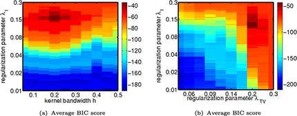
Figure 1: Plot of the $\operatorname{BIC}_{\mathrm{avg}}$ score over the regularization plane. The parameter vector $\theta^{t}$ is a smooth function of time and at each time point there is one observation. (a) The graph structure recovered using the method $\operatorname{smooth}$. (b) Recovered using the method $\operatorname{TV}$.

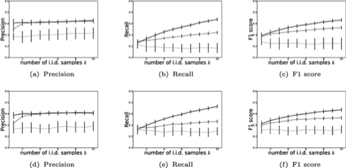
Figure 2: Results of estimation when the underlying parameter $\{\bolds{\theta}^{t}\}_{t\in\mathcal{T}_{n}}$ changes smoothly with time. The upper row consists of results when the graph is estimated combining the neighborhoods using the $\min$ operation, while the lower row consists of results when the $\max$ operation is used to combine neighborhoods. Precision, recall, and F1 score are plotted as the number of i.i.d. samples $k$ at each time point increases from 1 to 10. The solid, dashed, and dotted lines denote results for $\operatorname{smooth}$, $\operatorname{TV}$, and $\operatorname{static}$, respectively.

First, we discuss the estimation results when the underlying parameter vector changes smoothly. See Figure 2 for results. It can be seen that as the number of the i.i.d. observations at each time point increases, the performance of both methods smooth and TV increases. On the other hand, the performance of the method static does not benefit from additional i.i.d. observations. This observation should not be surprising as the time-varying network models better fit the data generating process. When the underlying parameter vector $\bolds{\theta}^{t}$ is a smooth function of time, we expect that the method smooth would have a faster convergence and better performance, which can be seen in Figure 2. There are some differences between the estimates obtained through MIN and MAX symmetrization. In our limited numerical experience, we have seen that MAX symmetrization outperforms MIN symmetrization. MIN symmetrization is more conservative in including edges to the graph and seems to be more susceptible to noise.

Next, we discuss the estimation results when then the underlying parameter vector is a piecewise constant function. See Figure 3 for results. Again, both performance of the method smooth and of the method TV improve as there are more independent samples at different time points, as opposed to the method static. It is worth noting that the empirical performance of smooth and TV is very similar in the setting when $\bolds{\theta}^{t}$ is a piecewise constant function of time, with the method TV performing marginally better. This may be a consequence of the way we present results, averaged over all time points in $\mathcal{T}_{n}$. A closer inspection of the estimated graphs shows that the method smooth poorly estimates graph structure close to the time point at which the parameter vector changes abruptly (results not shown).

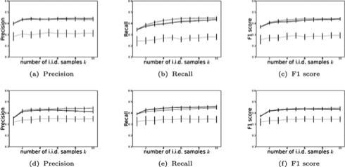
Figure 3: Results of estimation when the underlying parameter $\{\bolds{\theta}^{t}\}_{t\in\mathcal{T}_{n}}$ is a piecewise constant function of time. The upper row consists of results when the graph is estimated combining the neighborhoods using the $\min$ operation, while the lower row consists of results when the $\max$ operation is used to combine neighborhoods. Precision, recall, and F1 score are plotted as the number of i.i.d. samples $k$ at each time point increases from 1 to 10. The solid, dashed, and dotted lines denote results for $\operatorname{smooth}$, $\operatorname{TV}$, and $\operatorname{static}$, respectively.

We have decided to perform simulation studies on Erdös–Rényi graphs, while real-world graphs are likely to have different properties, such as a scale-free network with a long tail in its degree distribution. From a theoretical perspective (see Section 5), our method can still recover the true structure of these networks regardless of the degree distribution, although for a more complicated model, we may need more samples in order to achieve this. Peng et al. (2009) proposed a joint sparse regression model, which performs better than the neighborhood selection method when estimating networks with hubs (nodes with very high degree) and scale-free networks. For such networks, we can extend their model to our time-varying setting, and potentially make more efficient use of the samples, however, we do not pursue this direction here.

4 Applications to real data

In this section we present the analysis of two real data sets using the algorithms presented in Section 2. First, we present the analysis of the senate data consisting of Senators’ votes on bills during the 109th Congress. The second data set consists of expression levels of more than 4000 genes from the life cycle of Drosophila melanogaster.

4.1 Senate voting records data

The US senate data consists of voting records from 109th congress (2005–2006). There are 100 senators whose votes were recorded on the 542 bills. Each senator corresponds to a variable, while the votes are samples recorded as $-$1 for no and 1 for yes. This data set was analyzed in Banerjee, Ghaoui and d’Aspremont (2008), where a static network was estimated. Here, we analyze this data set in a time-varying framework in order to discover how the relationship between senators changes over time.

This data set has many missing values, corresponding to votes that were not cast. We follow the approach of Banerjee, Ghaoui and d’Aspremont (2008) and fill those missing values with ($-$1). Bills were mapped onto the $[0,1]$ interval, with 0 representing Jan 1st, 2005 and 1 representing Dec 31st, 2006. We use the Epanechnikov kernel for the method smooth. The tuning parameters are chosen optimizing the average BIC score over the same range as used for the simulations in Section 3. For the method smooth, the bandwidth parameter was selected as $h=0.174$ and the penalty parameter $\lambda_{1}=0.195$, while penalty parameters $\lambda_{1}=0.24$ and $\lambda_{\operatorname{TV}}=0.28$ were selected for the method TV. In the figures in this section, we use pink square nodes to represent republican Senators and blue circle nodes to represent democrat Senators.

A first question is whether the learned network reflects the political division between Republicans and Democrats. Indeed, at any time point $t$, the estimated network contains few clusters of nodes. These clusters consist of either Republicans or Democrats connected to each others; see Figure 4. Furthermore, there are very few links connecting different clusters. We observe that most Senators vote similarly to other members of their party. Links connecting different clusters usually go through senators that are members of one party, but have views more similar to the other party, for example, Senator Ben Nelson or Senator Chafee. Note that we do not necessarily need to estimate a time evolving network to discover this pattern of political division, as they can also be observed from a time-invariant network, for example, see Banerjee, Ghaoui and d’Aspremont (2008).

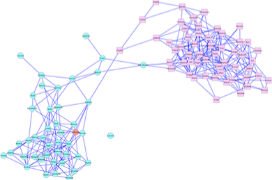
Figure 4: 109th Congress, Connections between Senators in April 2005. Democrats are represented with blue circles, Republicans with pink squares, and the red circle represents independent Senator Jeffords.

Therefore, what is more interesting is whether there is any time evolving pattern. To show this, we examine neighborhoods of Senators Jon Corzine and Bob Menendez. Senator Corzine stepped down from the Senate at the end of the 1st Session in the 109th Congress to become the Governor of New Jersey. His place in the Senate was filled by Senator Menendez. This dynamic change of interactions can be well captured by the time-varying network (Figure 5). Interestingly, we can see that Senator Lautenberg who used to interact with Senator Corzine switches to Senator Menendez in response to this event.

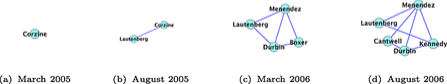
Figure 5: Direct neighbors of the node that represent Senator Corzine and Senator Menendez at four different time points. Senator Corzine stepped down at the end of the 1st Session and his place was taken by Senator Menendez, which is reflected in the graph structure.

Another interesting question is whether we can discover senators with swaying political stance based on time evolving networks. We discover that Senator Ben Nelson and Lincoln Chafee fall into this category. Although Senator Ben Nelson is a Democrat from Nebraska, he is considered to be one of the most conservative Democrats in the Senate. Figure 6 presents neighbors at distance two or less of Senator Ben Nelson at two time points, one during the 1st Session and one during the 2nd Session. As a conservative Democrat, he is connected to both Democrats and Republicans since he shares views with both parties. This observation is supported by Figure 6(a) which presents his neighbors during the 1st Session. It is also interesting to note that during the second session, his views drifted more toward the Republicans [Figure 6(b)]. For instance, he voted against abortion and withdrawal of most combat troops from Iraq, which are both Republican views.

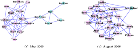
Figure 6: Neighbors of Senator Ben Nelson (distance two or lower) at the beginning of the 109th Congress and at the end of the 109th Congress. Democrats are represented with blue circles, Republicans with pink squares. The estimated neighborhood in August 2006 consists only of Republicans, which may be due to the type of bills passed around that time on which Senator Ben Nelson had similar views as other Republicans.

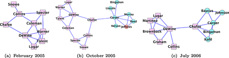
Figure 7: Neighbors of Senator Chafee (distance two or lower) at different time points during the 109th Congress. Democrats are represented with blue circles, Republicans with pink squares, and the red circle represents independent Senator Jeffords.

In contrast, although Senator Lincoln Chafee is a Republican, his political view grew increasingly Democratic. Figure 7 presents neighbors of Senator Chafee at three time points during the 109th Congress. We observe that his neighborhood includes an increasing amount of Democrats as time progresses during the 109th Congress. Actually, Senator Chafee later left the Republican Party and became an independent in 2007. Also, his view on abortion, gay rights, and environmental policies are strongly aligned with those of Democrats, which is also consistently reflected in the estimated network. We emphasize that these patterns about Senator Nelson and Chafee could not be observed in a static network.

4.2 Gene regulatory networks of Drosophila melanogaster

In this section we used the kernel reweighting approach to reverse engineer the gene regulatory networks of Drosophila melanogaster from a time series of gene expression data measured during its full life cycle. Over the developmental course of Drosophila melanogaster, there exist multiple underlying “themes” that determine the functionalities of each gene and their relationships to each other, and such themes are dynamical and stochastic. As a result, the gene regulatory networks at each time point are context-dependent and can undergo systematic rewiring, rather than being invariant over time. In a seminal study by Luscombe et al. (2004), it was shown that the “active regulatory paths” in the gene regulatory networks of Saccharomyces cerevisiae exhibit topological changes and hub transience during a temporal cellular process, or in response to diverse stimuli. We expect similar properties can also be observed for the gene regulatory networks of Drosophila melanogaster.

We used microarray gene expression measurements from Arbeitman et al. (2002) as our input data. In such an experiment, the expression levels of 4028 genes are simultaneously measured at various developmental stages. Particularly, 66 time points are chosen during the full developmental cycle of Drosophila melanogaster, spanning across four different stages, that is, embryonic (1–30 time point), larval (31–40 time point), pupal (41–58 time points), and adult stages (59–66 time points). In this study we focused on 588 genes that are known to be related to the developmental process based on their gene ontologies.

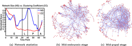
Figure 8: Characteristic of the dynamic networks estimated for the genes related to the developmental process. (a) Plot of two network statistics as functions of the development time line. Network size ranges between 1712 and 2061 over time, while local clustering coefficient ranges between 0.23 and 0.53 over time; To focus on relative activity over time, both statistics are normalized to the range between 0 and 1. (b) and (c) are the visualization of two examples of networks from different time points. We can see that network size can evolve in a very different way from the local clustering coefficient.

Usually, the samples prepared for microarray experiments are a mixture of tissues with possibly different expression levels. This means that microarray experiments only provide rough estimates of the average expression levels of the mixture. Other sources of noise can also be introduced into the microarray measurements during, for instance, the stage of hybridization and digitization. Therefore, microarray measurements are far from the exact values of the expression levels, and it will be more robust if we only consider the binary state of the gene expression: either being up-regulated or down-regulated. For this reason, we binarize the gene expression levels into $\{-1,1\}$ ($-$1 for down-regulated and 1 for up-regulated). We learned a sequence of binary MRFs from these time series.

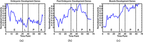
Figure 9: Interactivity of 3 groups of genes related to (a) embryonic development (ranging between 169 and 241), (b) post-embryonic development (ranging between 120 and 210), and (c) muscle development (ranging between 29 and 89). To focus on the relative activity over time, we normalize the score to $[0,1]$. The higher the interactivity, the more active the group of genes. The interactivities of these three groups are very consistent with their functional annotations.

First, we study the global pattern of the time evolving regulatory networks. In Figure 8(a) we plotted two different statistics of the reversed engineered gene regulatory networks as a function of the developmental time point (1–66). The first statistic is the network size as measured by the number of edges; and the second is the average local clustering coefficient as defined by Watts and Strogatz (1998). For comparison, we normalized both statistics to the range between $[0,1]$. It can be seen that the network size and its local clustering coefficient follow very different trajectories during the developmental cycle. The network size exhibits a wave structure featuring two peaks at mid-embryonic stage and the beginning of the pupal stage. A similar pattern of gene activity has also been observed by Arbeitman et al. (2002). In contrast, the clustering coefficients of the dynamic networks drop sharply after the mid-embryonic stage, and they stay low until the start of the adult stage. One explanation is that at the beginning of the development process, genes have a more fixed and localized function, and they mainly interact with other genes with similar functions. However, after mid-embryonic stage, genes become more versatile and involved in more diverse roles to serve the need of rapid development; as the organism turns into an adult, its growth slows down and each gene is restored to its more specialized role. To illustrate how the network properties change over time, we visualized two networks from mid-embryonic stage (time point 15) and mid-pupal stage (time point 45) using the spring layout algorithm in Figure 8(b) and (c) respectively. Although the size of the two networks are comparable, tight local clusters of interacting genes are more visible during mid-embryonic stage than mid-pupal stage, which is consistent with the evolution local clustering coefficient in Figure 8(a).

To judge whether the learned networks make sense biologically, we zoom into three groups of genes functionally related to different stages of the development process. In particular, the first group (30 genes) is related to embryonic development based on their functional ontologies; the second group (27 genes) is related to post-embryonic development; and the third group (25 genes) is related to muscle development. For each group, we use the number of within group connections plus all its outgoing connections to describe the activitiy of each group of genes (for short, we call it interactivity). In Figure 9 we plotted the time courses of interactivity for the three groups respectively. For comparison, we normalize all scores to the range of $[0,1]$. We see that the time courses have a nice correspondence with their supposed roles. For instance, embryonic development genes have the highest interactivity during embryonic stage, and post-embryonic genes increase their interactivity during the larval and pupal stages. The muscle development genes are less specific to certain developmental stages, since they are needed across the developmental cycle. However, we see its increased activity when the organism approaches its adult stage where muscle development becomes increasingly important.

The estimated networks also recover many known interactions between genes. In recovering these known interactions, the dynamic networks also provide additional information as to when interactions occur during development. In Figure 10 we listed these recovered known interactions and the precise time when they occur. This also provides a way to check whether the learned networks are biologically plausible given the prior knowledge of the actual occurrence of gene interactions. For instance, the interaction between genes msn and dock is related to the regulation of embryonic cell shape, correct targeting of photoreceptor axons. This is very consistent with the timeline provided by the dynamic networks. A second example is the interaction between genes sno and Dl which is related to the development of compound eyes of Drosophila. A third example is between genes caps and Chi which are related to wing development during pupal stage. What is most interesting is that the dynamic networks provide timelines for many other gene interactions that have not yet been verified experimentally. This information will be a useful guide for future experiments.

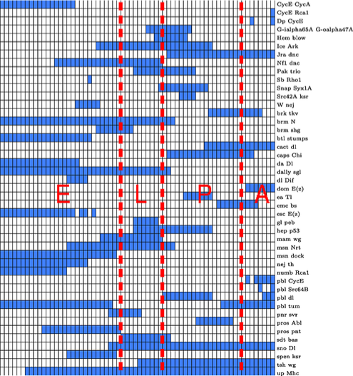
Figure 10: Timeline of 45 known gene interactions. Each cell in the plot corresponds to one gene pair of gene interaction at one specific time point. The cells in each row are ordered according to their time point, ranging from embryonic stage (E) to larval stage (L), to pupal stage (P), and to adult stage (A). Cells colored blue indicate the corresponding interaction listed in the right column is present in the estimated network; blank color indicates the interaction is absent.

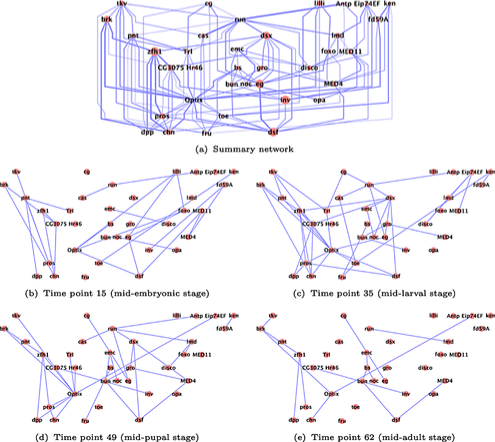
Figure 11: The largest transcriptional factors (TF) cascade involving 36 transcriptional factors. (a) The summary network is obtained by summing the networks from all time points. Each node in the network represents a transcriptional factor, and each edge represents an interaction between them. On different stages of the development, the networks are different, (b), (c), (d), (e) shows representative networks for the embryonic, larval, pupal, and adult stage of the development respectively.

We further studied the relations between 130 transcriptional factors (TF). The network contains several clusters of transcriptional cascades, and we will present the detail of the largest transcriptional factor cascade involving 36 transcriptional factors (Figure 11). This cascade of TFs is functionally very coherent, and many TFs in this network play important roles in the nervous system and eye development. For example, Zn finger homeodomain 1 (zhf1), brinker (brk), charlatan (chn), decapentaplegic (dpp), invected (inv), forkhead box, subgroup 0 (foxo), Optix, eagle (eg), prospero (pros), pointed (pnt), thickveins (tkv), extra macrochaetae (emc), lilliputian (lilli), and doublesex (dsx) are all involved in nervous and eye development. Besides functional coherence, the network also reveals the dynamic nature of gene regulation: some relations are persistent across the full developmental cycle, while many others are transient and specific to certain stages of development. For instance, five transcriptional factors, brk-pnt-zfh1-pros-dpp, form a long cascade of regulatory relations which are active across the full developmental cycle. Another example is gene Optix which is active across the full developmental cycle and serves as a hub for many other regulatory relations. As for transience of the regulatory relations, TFs to the right of the Optix hub reduced in their activity as development proceeds to a later stage. Furthermore, Optix connects two disjoint cascades of gene regulations to its left and right side after embryonic stage.

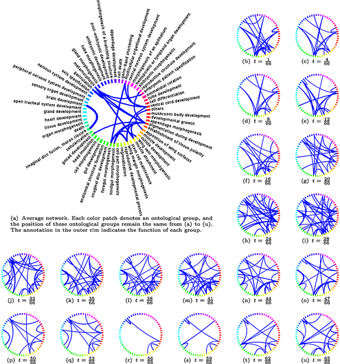
Figure 12: Interactions between gene ontological groups related to the developmental process undergo dynamic rewiring. The weight of an edge between two ontological groups is the total number of connections between genes in the two groups. In the visualization, the width of an edge is proportional to its edge weight. We thresholded the edge weight at 30 in (b)–(u) so that only those interactions exceeding this number are displayed. The average network in (a) is produced by averaging the networks underlying (b)–(u). In this case, the threshold is set to 20 instead.

The dynamic networks also provide an overview of the interactions between genes from different functional groups. In Figure 12 we grouped genes according to 58 ontologies and visualized the connectivity between groups. We can see that large topological changes and network rewiring occur between functional groups. Besides expected interactions, the figure also reveals many seemingly unexpected interactions. For instance, during the transition from pupa stage to adult stage, Drosophila is undergoing a huge metamorphosis. One major feature of this metamorphosis is the development of the wing. As can be seen from Figure 12(r) and (s), genes related to metamorphosis, wing margin morphogenesis, wing vein morphogenesis, and apposition of wing surfaces are among the most active group of genes, and they carry their activity into adult stage. Actually, many of these genes are also very active during early embryonic stage [for example, Figure 12(b) and (c)]; though the difference is they interact with different groups of genes. On one hand, the abundance of the transcripts from these genes at embryonic stage is likely due to maternal deposit (Arbeitman et al., 2002); on the other hand, this can also be due to the diverse functionalities of these genes. For instance, two genes related to wing development, held out wings (how) and tolloid (td), also play roles in embryonic development.

5 Some properties of the algorithms

In this section we discuss some theoretical guarantees of the proposed algorithms. The most challenging aspect in estimating time-varying graphs is that the dimension of the data $p$ can be much larger than the size of the sample $n$ ($p\gg n$), and there is usually only one sample per time point. For example, in a genome-wide reverse engineering task, the number of genes can be well over ten thousand ($p>10{,}000$), while the total number of microarray measurements is only in the hundreds ($n\sim 100$) and the measurements are collected at different developmental stages. Then, the question is what are the sufficient conditions under which our algorithms recover the sequence of unknown graphs $\{G^{t}\}_{t\in\mathcal{T}_{n}}$ correctly.

To provide asymptotic results, we will consider the model dimension $p$ to be an increasing function of the sample size $n$, and characterize the scaling of $p$ with respect to $n$ under which structure recovery is possible. Furthermore, we will assume the following:

1. The graphs $\{G^{t}\}_{t\in\mathcal{T}_{n}}$ are sparse, that is, the maximum node degree $s$ of a graph is upper bounded and much smaller than the sample size $n$ ($s\ll n$). The intuition here is that the sparsity of a graph is positively correlated with the complexity of a model; a sparse graph effectively limits the degree of freedom of the model, which makes structure recovery possible given a small sample size.

2. When regressing $X_{u}$ on $\mathbf{X}_{\setminus u}$, the relevant covariates $S^{\tau}(u)$ should not be overly dependent on each other. We need this assumption for the model to be identifiable. Intuitively, if two covariates are very strongly correlated with each other, we would not be able to distinguish one from another.

3. The dependencies between irrelevant covariates $S^{\tau,c}(u)$ and those relevant ones $S^{\tau}(u)$ are not too strong. Similar to the assumption 2, we need this assumption for the model to be identifiable. Intuitively, if an irrelevant covariate looks very similar to a relevant covariate, it will be hard for an algorithm to tell which one is the true covariate. Assumptions 2 and 3 are common in other work on sparse estimation, for example, Wainwright (2009); Meinshausen and Bühlmann (2006); Ravikumar, Wainwright and Lafferty (2010).

4. The minimum parameter value $\theta_{\min}:=\min_{t\in\mathcal{T}_{n}}\min_{v\in S^{t}(u)}|\theta_{uv}^{t}|$ is bounded away from zero. This assumption is required in order to separate nonzero parameters from zero parameters. If a covariate has very small effect on the output, then it will be hard for the algorithm to distinguish it from noise.

5. The parameter vector $\bolds{\theta}^{t}$ is a smooth function of time. This guarantees that the graphical models at adjacent time points are similar enough such that we can borrow information across time point by reweighting the observations. Under this assumption, the method smooth is able to achieve sufficiently fast convergence rates for each neighborhood estimate; then the consistency of the overall graph estimation can be achieved by an application of the union bound over all nodes $u\in V$.

6. The kernel function $K(\cdot)$ is a symmetric nonnegative function with a bounded support on $[-1,1]$. This assumption is needed for technical reasons, and it gives some regularity conditions on the kernel used to define the weights.

With these assumptions, we can state the following theorem for algorithm smooth [a complete statement of assumptions 1–6 and the proof of the theorem are given in Kolar and Xing (2009)]:

Theorem 1 ((Kolar and Xing, 2009))

Assume that assumptions 1 to 6 given above hold. Let the regularization parameter satisfy

$$\lambda_{1}\geq C\frac{\sqrt{\log p}}{n^{1/3}}$$

for a constant $C>0$ independent of $(n,p,s)$. Furthermore, assume that the following conditions hold:

1. $h=\mathcal{O}(n^{-1/3})$,

2. $s=o(n^{1/3})$, $\frac{s^{3}\log p}{n^{2/3}}=o(1)$,

3. $\theta_{\min}=\Omega(\frac{\sqrt{s\log p}}{n^{1/3}}).$

Then for any $\tau\in\mathcal{T}_{n}$, the method smooth estimates a graph $\hat{G}^{\tau}$ that satisfies

$$\mathbb{P}[\hat{G}^{\tau}\neq G^{\tau}]=\mathcal{O}\biggl{(}\exp\biggl{(}-C\frac{n^{2/3}}{s^{3}}+C^{\prime}\log p\biggr{)}\biggr{)}\rightarrow 0,$$ (16)

for some constants $C^{\prime},C^{\prime\prime}$ independent of $(n,p,s)$.

The theorem means that the procedure can recover the graph asymptotically by using appropriate regularization parameter $\lambda_{1}$, as long as both the model dimension $p$ and the maximum node degree $s$ are not too large, and the minimum parameter value $\theta_{\min}$ does not tend to zero too fast. In particular, the model dimension is allowed to grow as $p=\mathcal{O}(\exp(n^{\xi}))$ for some $\xi<2/3$, when $s=\mathcal{O}(1)$ as is commonly assumed. The consistency of the structure recovery is a somewhat surprising result since at any time point there is at most one available sample corresponding to each graph.

Currently we do not have a consistency result for the estimator produced by the method TV, however, we have obtained some insight on how to solve this problem and plan to pursue it in our future research. The main difficulty seems to be the presence of both the $\ell_{1}$ and $\operatorname{TV}(\cdot)$ regularization terms in equation (10), which complicates the analysis. However, if we relate the method TV to the problem of multiple change point detection, we can observe the following: the $\operatorname{TV}(\cdot)$ penalty biases the estimate $\{\hat{\bolds{\theta}}{}^{t}\}_{t\in\mathcal{T}_{n}}$ toward a piecewise constant solution, and this effectively partitions the time interval $[0,1]$ into segments within which the parameter is constant. If we can estimate the partition $\mathcal{B}_{u}$ correctly, then the graph structure can also be estimated successfully if there are enough samples on each segment of the partition. In fact, Rinaldo (2009) observed that it is useful to consider a two-stage procedure in which the first stage uses the total variation penalty to estimate the partition, and the second stage then uses the $\ell_{1}$ penalty to determine nonzero parameters within each segment. Although his analysis is restricted to the fused lasso (Tibshirani et al., 2005), we believe that his techniques can be extended for analyzing our method TV. Besides assumptions 1 to 4 which appeared in method smooth, additional assumptions may be needed to assure the consistent estimation of the partition $\mathcal{B}_{u}$.

6 Discussion

We have presented two algorithms for an important problem of structure estimation of time-varying networks. While the structure estimation of the static networks is an important problem in itself, in certain cases static structures are of limited use. More specifically, a static structure only shows connections and interactions that are persistent throughout the whole time period and, therefore, time-varying structures are needed to describe dynamic interactions that are transient in time. Although the algorithms presented in this paper for learning time-varying networks are simple, they can already be used to discover some patterns that would not be discovered using a method that estimates static networks. However, the ability to learn time-varying networks comes at a price of extra tuning parameters: the bandwidth parameter $h$ or the penalty parameter $\lambda_{\operatorname{TV}}$.

Throughout the paper, we assume that the observations at different points in time are independent. An important future direction is the analysis of the graph structure estimation from a general time series, with dependent observations. In our opinion, this extension will be straightforward but with great practical importance. Furthermore, we have worked with the assumption that the data are binary, however, extending the procedure to work with multi-category data is also straightforward. One possible approach is explained in Ravikumar, Wainwright and Lafferty (2010) and can be directly used here.

There are still ways to improve the methods presented here. For instance, more principled ways of selecting tuning parameters are definitely needed. Selecting the tuning parameters in the neighborhood selection procedure for static graphs is not an easy problem, and estimating time-varying graphs makes the problem more challenging. Furthermore, methods presented here do not allow for the incorporation of existing knowledge on the network topology into the algorithm. In some cases, the data are very scarce and we would like to incorporate as much prior knowledge as possible, so developing Bayesian methods seems very important.

The method smooth and the method TV represent two different ends of the spectrum: one algorithm is able to estimate smoothly changing networks, while the other one is tailored toward estimation of structural changes in the model. It is important to bring the two methods together in the future work. There is a great amount of work on nonparametric estimation of change points and it would be interesting to incorporate those methods for estimating time-varying networks.

References

- Arbeitman et al. (2002) Arbeitman, M., Furlong, E., Imam, F., Johnson, E., Null, B., Baker, B., Krasnow, M., Scott, M., Davis, R. and White, K. (2002). Gene expression during the life cycle of Drosophila melanogaster. Science 297 2270–2275.
- Banerjee, Ghaoui and d’Aspremont (2008) Banerjee, O., El Ghaoui, L. and d’Aspremont, A. (2008). Model selection through sparse maximum likelihood estimation. J. Mach. Learn. Res. 9 485–516. \MR2417243
- Bresler, Mossel and Sly (2008) Bresler, G., Mossel, E. and Sly, A. (2008). Reconstruction of Markov random fields from samples: Some observations and algorithms. In APPROX ’08 / RANDOM ’08: Proceedings of the 11th International Workshop, APPROX 2008, and 12th International Workshop, RANDOM 2008 on Approximation, Randomization and Combinatorial Optimization 343–356. Springer, Berlin.
- Davidson (2001) Davidson, E. H. (2001). Genomic Regulatory Systems. Academic Press, San Diego.
- Drton and Perlman (2004) Drton, M. and Perlman, M. D. (2004). Model selection for Gaussian concentration graphs. Biometrika 91 591–602. \MR2090624
- Duchi, Gould and Koller (2008) Duchi, J., Gould, S. and Koller, D. (2008). Projected subgradient methods for learning sparse Gaussians. In Proceedings of the Twenty-fourth Conference on Uncertainty in AI (UAI) 145–152.
- Efron et al. (2004) Efron, B., Hastie, T., Johnstone, I. and Tibshirani, R. (2004). Least angle regression. Ann. Statist. 32 407–499. \MR2060166
- Fan and Li (2001) Fan, J. and Li, R. (2001). Variable selection via nonconcave penalized likelihood and its oracle properties. J. Amer. Statist. Assoc. 96 1348–1360. \MR1946581
- Fan, Feng and Wu (2009) Fan J., Feng Y. and Wu, Y. (2009). Network exploration via the adaptive LASSO and SCAD penalties. Ann. Appl. Statist. 3 521–541.
- Friedman, Hastie and Tibshirani (2007) Friedman, J., Hastie, J. and Tibshirani, R. (2007). Sparse inverse covariance estimation with the graphical lasso. Biostat, kxm045. Available at http://biostatistics.oxfordjournals.org/cgi/content/abstract/kxm045v1.
- Friedman, Hastie and Tibshirani (2008) Friedman, J., Hastie, T. and Tibshirani, R. (2008). Regularization paths for generalized linear models via coordinate descent. Technical report, Dept. Statistics, Stanford Univ.
- Friedman et al. (2007) Friedman, J., Hastie, T., Hofling, H. and Tibshirani, R. (2007). Pathwise coordinate optimization. Ann. Appl. Statist. 1 302. \MR2415737
- Getoor and Taskar (2007) Getoor, L. and Taskar, B. (2007). Introduction to Statistical Relational Learning (Adaptive Computation and Machine Learning). MIT Press, Cambridge, MA. \MR2391486
- Grant and Boyd (2008) Grant, M. and Boyd, S. (2008). Cvx: Matlab software for disciplined convex programming (web page and software). Available at http://stanford.edu/~boyd/cvx.
- Guo et al. (2007) Guo, F., Hanneke, S., Fu, W. and Xing, E. P. (2007). Recovering temporally rewiring networks: A model-based approach. In Proceedings of the 24th International Conference on Machine Learning 321–328. ACM Press, New York.
- Hanneke and Xing (2006) Hanneke, S. and Xing E. P. (2006). Discrete temporal models of social networks. Lecture Notes in Computer Science 4503 115–125.
- Koh, Kim and Boyd (2007) Koh, K., Kim, S.-J. and Boyd, S. (2007). An interior-point method for large-scale l1-regularized logistic regression. J. Mach. Learn. Res. 8 1519–1555. \MR2332440
- Kolar and Xing (2009) Kolar, R. and Xing, E. P. (2009). Sparsistent estimation of time-varying discrete Markov random fields. ArXiv e-prints.
- Lauritzen (1996) Lauritzen, S. L. (1996). Graphical Models. Oxford Univ. Press, Oxford. \MR1419991
- Luscombe et al. (2004) Luscombe, N., Babu, M., Yu, H., Snyder, M., Teichmann, S. and Gerstein, M. (2004). Genomic analysis of regulatory network dynamics reveals large topological changes. Nature 431 308–312.
- Meinshausen and Bühlmann (2006) Meinshausen, N. and Bühlmann, P. (2006). High-dimensional graphs and variable selection with the lasso. Ann. Statist. 34 1436. \MR2278363
- Peng et al. (2009) Peng, J., Wang, P., Zhou, N. and Zhu, J. (2009). Partial correlation estimation by joint sparse regression models. J. Amer. Statist. Assoc. 104 735–746. \MR2541591
- Ravikumar, Wainwright and Lafferty (2010) Ravikumar, P., Wainwright, M. J. and Lafferty, J. D. (2010). High-dimensional ising model selection using regularized logistic regression. Ann. Statist. 38 1287–1319.
- Rinaldo (2009) Rinaldo, A. (2009). Properties and refinements of the fused lasso. Ann. Statist. 37 2922–2952. \MR2541451
- Rothman et al. (2008) Rothman, A. J., Bickel, P. J., Levina, E. and Zhu, J. (2008). Sparse permutation invariant covariance estimation. Electron. J. Statist. 2 494. \MR2417391
- Sarkar and Moore (2006) Sarkar, P. and Moore, A. (2006). Dynamic social network analysis using latent space models. SIGKDD Explor. Newsl. 7 31–40.
- Tibshirani et al. (2005) Tibshirani, R., Saunders, M., Rosset, S., Zhu, J. and Knight, K. (2005). Sparsity and smoothness via the fused lasso. J. Roy. Statist. Soc. Ser. B 67 91–108. \MR2136641
- Tseng (2001) Tseng, P. (2001). Convergence of a block coordinate descent method for nondifferentiable minimization. J. Optim. Theory Appl. 109 475–494. \MR1835069
- van Duijn, Gile and Handcock (2009) van Duijn, M. A. J., Gile, K. J. and Handcock, M. S. (2009). A framework for the comparison of maximum pseudo-likelihood and maximum likelihood estimation of exponential family random graph models. Social Networks 31 52–62.
- Wainwright and Jordan (2008) Wainwright, M. J. and Jordan, M. I. (2008). Graphical models, exponential families, and variational inference. Found. Trends Mach. Learn. 1 1–305.
- Wainwright (2009) Wainwright, M. J. (2009). Sharp thresholds for high-dimensional and noisy sparsity recovery using -constrained quadratic programming (lasso). IEEE Trans. Inform. Theory 55 2183–2202.
- Watts and Strogatz (1998) Watts, D. and Strogatz, S. (1998). Collective dynamics of ‘small-world’ networks. Nature 393 440–442.
- Yuan and Lin (2007) Yuan, M. and Lin, Y. (2007). Model selection and estimation in the Gaussian graphical model. Biometrika 94 19–35. \MR2367824
- Zhou, Lafferty and Wasserman (2008) Zhou, S., Lafferty, J. and Wasserman, L. (2008). Time varying undirected graphs. In Conference on Learning Theory (R. A. Servedio and T. Zhang, eds.) 455–466. Omnipress, Madison, WI.
- Zou and Li (2008) Zou, H. and Li, R. (2008). One-step sparse estimates in nonconcave penalized likelihood models. Ann. Statist. 36 1509. \MR2435443