Rigorous treatment of electrostatics for spatially varying dielectrics based on energy minimization

Abstract

A novel energy minimization formulation of electrostatics that allows computation of the electrostatic energy and forces to any desired accuracy in a system with arbitrary dielectric properties is presented. An integral equation for the scalar charge density is derived from an energy functional of the polarization vector field. This energy functional represents the true energy of the system even in non-equilibrium states. Arbitrary accuracy is achieved by solving the integral equation for the charge density via a series expansion in terms of the equation’s kernel, which depends only on the geometry of the dielectrics. The streamlined formalism operates with volume charge distributions only, not resorting to introducing surface charges by hand. Therefore, it can be applied to any spatial variation of the dielectric susceptibility, which is of particular importance in applications to biomolecular systems. The simplicity of application of the formalism to real problems is shown with analytical and numerical examples.

I Introduction

Molecular dynamics (MD) simulations of solute-solvent systems in chemistry and biology require accurate computation of electrostatic forces in order to obtain meaningful results. For practical purposes, computational efficiency is also essential, and various formulations exist that strive to achieve a balance between these two requirements. The explicit solvent methods simulate behaviour of each single solvent molecule which may be prohibitively expensive for a system of reasonable dimensions. In addition to having high computational costs, explicit solvent methods are usually tailored for reproducing one of the many physical properties of the solvent and therefore may not be well suited for a general description of solute-solvent systems (see Wallqvist ; Tirado-Rives ; Guillot for reviews and performance analyses).

The alternative approach is to treat the solvent as a dielectric continuum, and the solute as a different dielectric object in the solvent. The dielectric properties of the solvent and the solute usually serve as parameters of the model. In the literature this scheme is known as the implicit or continuum solvent method (for reviews see BrooksIII ; Honig ; Tomasi1 ; Cramer ; Bashford ). Computations based on these methods are inherently faster while comparable in accuracy with those using explicit methods, at least in the situations when interactions between solute and solvent molecules can be neglected. For reasons of computational efficiency, many of the implemented implicit solvent methods make use of assumptions which prevent improvement in accuracy even as computational resources increase. The so-called generalized Born model is a good example of such uncontrolled approximations (see Doerr for a discussion).

To achieve controllable accuracy, we have recently proposed a novel scheme Doerr based on determining surface charges satisfying the displacement field boundary condition. With this scheme, one can achieve any level of accuracy permitted by the available computing power, while remaining computationally more efficient than explicit solvent methods. The main idea is to treat the induced surface charges at the boundaries as the variables to be solved for. This makes the potential, expressed directly in terms of the induced surface charge density, continuous at the boundary. Therefore only the displacement field boundary condition remains, and it leads to a set of algebraic equations for the surface charge densities. The potential is obtained at no additional cost.

One of the seeming oversimplifications in the implicit solvent methods is the assumption of a sharp boundary between the solute and solvent. It is known, for example, that the solute (e.g., proteins) may strongly interact with the surrounding solvent molecules producing the so-called hydration layer(s) Bagchi . To determine electrostatic forces acting on a protein coated with such hydration layers, one needs to find induced charges in a spatially varying dielectric medium. In this paper we develop a rigorous framework, based on functional minimization, for handling spatially varying dielectrics.

Functional variation is a powerful approach in modern physics. Despite common use in quantum electrodynamics, variational techniques in classical electrostatics are relatively rare and focus mainly on boundary value problems for linear dielectrics Schwinger2 . It has long been a textbook fact that the true electrostatic potential minimizes the system’s energy for a given configuration of charges Jackson . A suitable energy functional can be constructed in general for any system of continuous media including systems with inhomogeneous and nonlinear dielectric properties. For instance, free energy functionals became an important tool in description of electrolyte solutions within the mean-field (Poisson-Boltzmann) approach (see a recent paper McCammon and references therein).

From our viewpoint the electrostatic potential is not the best choice for a minimization variable as it contains information about both the cause and effect, i.e. the source and induced charge densities. Moreover constitutive relations must be assumed (as in Allen ). And finally this approach depends on prior knowledge of the Green’s function with boundary conditions suitable for the given problem. In contrast, we use the polarization as the fundamental function as was proposed by Marcus over fifty years ago Marcus , albeit with a different functional. The constitutive relations are then obtained as a result of minimization of the energy functional. The only boundary condition needed is that the potential goes to zero sufficiently rapidly (like inverse of the distance) at large distances.

In Marcus’s formulation Marcus , the electric field and electric polarization were strongly motivated as the vectors defining the electric state of the system. This formulation was aimed at the processes (charge transfer chemical reactions) which happen on a much shorter time scale than the molecular rearrangement in response to the changing electric field. Marcus attempted to deal with this problem by dividing the polarization into a fast reacting part that is proportional to the local electric field and slowly reacting part that is not a function of the local electric field. As a result, the free energy functional derived by Marcus contains several electric fields and polarizations of various origins.

A physically sound free energy functional was proposed by Felderhof Felderhof in the context of a discussion of thermal fluctuations of the polarization and magnetization in dielectric magnetic media. However, a free energy of this type seems not to have been adopted for calculation of electrostatic fields until recently. An example of numerical implementation using Felderhof’s scheme can be found in Levy . There, the polarization vector field was expanded in a plane waves basis set. The energy functional is then an ordinary function of the expansion coefficients which, in turn, become the variational parameters of a standard multidimensional optimization problem. Fast Fourier transforms were used to go from the real space to the reciprocal space representations.

An approach close to Felderhof’s scheme was also taken in Attard where a thermodynamic functional was constructed with the polarization as the independent function. However, the techniques used there are suitable for systems with sharp boundaries only (the susceptibility is not considered to be a function of coordinates, but is rather treated as a piecewise constant).

In this paper we construct an energy minimization scheme suitable for a rigorous treatment of systems with spatially varying dielectric functions, be they linear or nonlinear. In the case of linear dielectrics, our functional is equivalent to that proposed by Felderhof Felderhof . In section II we give the details of the formulation and describe a systematic protocol for obtaining the total charge density. To show the versatility of the scheme we apply it in section III to systems with sharp boundaries for which the exact solutions (or the exact equations governing the exact solutions) are known. In section IV we present numerical results for the case of two interacting dielectric charged spheres (solutes) placed in a dielectric solvent. We discuss the differences in force and energy between the situations with sharp and smooth boundaries. Finally we conclude with a discussion assessing the usefulness of the method. Electrostatic CGS units are used throughout.

II Fundamental Formulation

Polarization is the response of a dielectric medium to an applied electric field. The phenomenon is usually visualized as the appearance of an induced dipole moment due to a small shift in the relative positions of the positive and negative charge centers at the atomic scale Feynman . The shift may be either translational or rotational or both, depending on the quantum mechanical and electromagnetic interactions at the atomic level. The applied electric fields must be weak enough not to split the atoms or molecules into their constituents. The system is in a state of equilibrium under the external electromagnetic and the intrinsic restoring forces.

Quantitatively, polarization ${{\rm\bf P}}({{\rm\bf r}})$ is the density of induced dipole moment at location ${{\rm\bf r}}$. This density in classical electrodynamics is defined through averaging of dipole moments of constituent atoms/molecules in a small volume centered around ${{\rm\bf r}}$. The amount of polarization depends on the applied force and the susceptibility of the medium to such forces. Determination of the susceptibility of the medium (or rather the intrinsic restoring force in the medium) is the subject of quantum mechanics rather than classical electrodynamics. Polarization is thus a classical/macroscopic variable summarizing quantum mechanical effects at the atomic/microscopic level. Therefore, we choose the polarization vector field ${{\rm\bf P}}({{\rm\bf r}})$ and electric field ${{\rm\bf E}}({{\rm\bf r}})$, in contrast to the more commonly used pair ${{\rm\bf E}}({{\rm\bf r}})$ and ${{\rm\bf D}}({{\rm\bf r}})$, as our fundamental variables. This choice provides a simpler connection to the parameters determined in microscopic physics.

We express the energy as a functional $U[{{\rm\bf P}}]$

$$U[{{\rm\bf P}}]=U_{\rm C}[{{\rm\bf P}}]+W[{{\rm\bf P}}],$$ (1)

where $U_{\rm C}[{{\rm\bf P}}]$ is the electrostatic energy of interaction of all charges present in the system, and $W[{{\rm\bf P}}]$ is the energy required to create the given polarization vector field ${{\rm\bf P}}({{\rm\bf r}})$.

From simple considerations it can be shown Feynman ; Landau that the variation of polarization in the vicinity of a point is equivalent to the presence of an induced charge density ${\rho_{\rm i}}({{\rm\bf r}})=-\nabla\cdot{{\rm\bf P}}({{\rm\bf r}})$. Therefore, the total charge density ${\rho_{\rm t}}({{\rm\bf r}})$ in the medium is a sum of the free charge density ${\rho_{\rm f}}({{\rm\bf r}})$ and ${\rho_{\rm i}}({{\rm\bf r}})$:

$${\rho_{\rm t}}({\rm\bf r})={\rho_{\rm f}}({\rm\bf r})+{\rho_{\rm i}}({\rm\bf r}).$$ (2)

Then

$$U_{\rm C}[{{\rm\bf P}}]=\frac{1}{2}\int\left[{\rho_{\rm f}}({{\rm\bf r}})-\nabla\cdot{{\rm\bf P}}({{\rm\bf r}})\right]\frac{1}{|{{\rm\bf r}}-{{\rm\bf r}}^{\prime}|}\left[{\rho_{\rm f}}({{\rm\bf r}}^{\prime})-\nabla\cdot{{\rm\bf P}}({{\rm\bf r}}^{\prime})\right]d{{\rm\bf r}}d{{\rm\bf r}}^{\prime}.$$ (3)

Note first that we do not include any separate term for induced surface charges as was done in some of the earlier formulations of functional minimization Marcus ; Attard . The volume charge density is the most general form of charge density possible. Secondly, (3) is the Coulomb energy in vacuum and hence quite fundamental as opposed to the form with the dielectric constant of the material in the denominator used in some of the earlier works Attard .

The work functional $W[{{\rm\bf P}}]$ should contain the intrinsic self interaction of the polarization vector field. Here we consider only local contact terms for the intrinsic interactions. Noting that the energy functional is a scalar and assuming ${{\rm\bf P}}\leftrightarrow-{{\rm\bf P}}$ symmetry, one can write the general work functional $W[{{\rm\bf P}}]$ as a polynomial expansion in even powers of ${{\rm\bf P}}$ (or the components $P_{i}$). Thus we may write,

$$W[{{\rm\bf P}}]=\frac{1}{2}\int\left[P_{i}\,\left(\frac{1}{\chi({{\rm\bf r}})}\right)_{ij}\,P_{j}+P_{i}P_{j}\,\left(\frac{1}{\mu({{\rm\bf r}})}\right)_{ijkl}\,P_{k}P_{l}+\cdots\right]d{{\rm\bf r}},$$ (4)

where the interaction tensors $1/\chi$, $1/\mu$, etc. describe the linear and nonlinear dielectric properties of the media, isotropic or anisotropic (summation over repeated indices is assumed). The effective dielectric properties of the medium at the macroscopic level are now contained in these quantities.

We emphasize that $U[{{\rm\bf P}}]$ is the actual energy functional unlike various other functionals proposed in the literature Jackson ; Allen ; McCammon ; Briggs which yield the energy or free energy of the system only at equilibrium. The equilibrium distribution of polarization (as well as induced charge distribution) can be obtained by minimizing this energy functional with respect to the polarization. For any given external charge distribution and spatially varying dielectric susceptibilities one can obtain the solution analytically or numerically.

We may truncate the series in (4) at an order suitable for the problem at hand. For example, if the field is very weak we can retain only the quadratic term which corresponds to the case of linear dielectrics (isotropy is also assumed for the sake of simplicity of presentation):

$$U[{{\rm\bf P}}]=U_{C}[{{\rm\bf P}}]+\frac{1}{2}\int\frac{{{\rm\bf P}}({{\rm\bf r}})\cdot{{\rm\bf P}}({{\rm\bf r}})}{\chi({{\rm\bf r}})}d{{\rm\bf r}}.$$ (5)

Performing a functional variation with respect to the polarization vector ${{\rm\bf P}}$, we arrive at an integro-differential equation defining the equilibrium polarization

$$\frac{{{\rm\bf P}}({{\rm\bf r}})}{\chi({{\rm\bf r}})}+\nabla_{{\rm\bf r}}\int\frac{{\rho_{\rm f}}({{\rm\bf r}}^{\prime})-\nabla\cdot{{\rm\bf P}}({{\rm\bf r}}^{\prime})}{|{{\rm\bf r}}-{{\rm\bf r}}^{\prime}|}d{{\rm\bf r}}^{\prime}=0$$ (6)

which implies

$${{\rm\bf P}}({{\rm\bf r}})=\chi({{\rm\bf r}})\int\left[{\rho_{\rm f}}({{\rm\bf r}}^{\prime})-\nabla\cdot{{\rm\bf P}}({{\rm\bf r}}^{\prime})\right]\frac{{{\rm\bf r}}-{{\rm\bf r}}^{\prime}}{|{{\rm\bf r}}-{{\rm\bf r}}^{\prime}|^{3}}d{{\rm\bf r}}^{\prime}=\chi({{\rm\bf r}}){{\rm\bf E}}({{\rm\bf r}})\;.$$ (7)

Thus the constitutive relation for a linear dielectric is obtained as a result of functional minimization, with the expansion coefficient $\chi({{\rm\bf r}})$ turning out to be the dielectric susceptibility. Inserting the equilibrium polarization (7) in (5) results in the well known expression for the total energy of the system:

$$U=\frac{1}{2}\int{\rho_{\rm f}}({{\rm\bf r}})\frac{1}{|{{\rm\bf r}}-{{\rm\bf r}}^{\prime}|}\left[{\rho_{\rm f}}({{\rm\bf r}}^{\prime})-\nabla\cdot{{\rm\bf P}}({{\rm\bf r}}^{\prime})\right]d{{\rm\bf r}}d{{\rm\bf r}}^{\prime}.$$ (8)

Keeping two (or more) terms in the series (4) introduces nonlinearity into the problem. The energy functional in this case is given by

$$U[{{\rm\bf P}}]=U_{C}[{{\rm\bf P}}]+\frac{1}{2}\int\frac{{{\rm\bf P}}({{\rm\bf r}})\cdot{{\rm\bf P}}({{\rm\bf r}})}{\chi({{\rm\bf r}})}d{{\rm\bf r}}+\frac{1}{2}\int\frac{\left[{{\rm\bf P}}({{\rm\bf r}})\cdot{{\rm\bf P}}({{\rm\bf r}})\right]^{2}}{\mu({{\rm\bf r}})}d{{\rm\bf r}}\;.$$ (9)

Performing a functional variation as above we now obtain

$${{\rm\bf P}}({{\rm\bf r}})=\chi({{\rm\bf r}}){{\rm\bf E}}({{\rm\bf r}})-2\frac{\chi({{\rm\bf r}})}{\mu({{\rm\bf r}})}\left[{{\rm\bf P}}({{\rm\bf r}})\cdot{{\rm\bf P}}({{\rm\bf r}})\right]{{\rm\bf P}}({{\rm\bf r}})\;.$$ (10)

Given that the first term on the right hand side is the dominant one, we can obtain the solution via iteration. The first approximation would be the same as the result for the linear dielectrics. Substituting it back into (10), we obtain at the second order of approximation,

$${{\rm\bf P}}({{\rm\bf r}})=\chi({{\rm\bf r}}){{\rm\bf E}}({{\rm\bf r}})-2\frac{\chi^{4}({{\rm\bf r}})}{\mu({{\rm\bf r}})}\left[{{\rm\bf E}}({{\rm\bf r}})\cdot{{\rm\bf E}}({{\rm\bf r}})\right]{{\rm\bf E}}({{\rm\bf r}})\;.$$ (11)

One can continue with this to obtain a series of terms with higher and higher powers of $[{{\rm\bf E}}\cdot{{\rm\bf E}}]$. This gives the desired result for nonlinear dielectrics. We should mention once more that this solution is true for weak fields so that the higher order terms are successively weaker. To ensure this condition we require $\mu({{\rm\bf r}})>>\chi^{3}({{\rm\bf r}})$ to be true to any order of approximation.

Let us now solve (7) for the case of linear dielectrics. We simplify the analysis by choosing the (scalar) induced density ${\rho_{\rm i}}=-\nabla\cdot{\bf P}$ as our variable.

Using the relation

$$\nabla_{{\rm\bf r}}\cdot\left[{{{\rm\bf r}}-{{\rm\bf r}}^{\prime}\over|{{\rm\bf r}}-{{\rm\bf r}}^{\prime}|^{3}}\right]=4\pi\delta({{\rm\bf r}}-{{\rm\bf r}}^{\prime})\;,$$ (12)

we obtain from (7)

$$\nabla\cdot{\rm\bf P}({\rm\bf r})=\nabla\chi({\rm\bf r})\cdot\int{{\rm\bf r}-{\rm\bf r}^{\prime}\over|{\rm\bf r}-{\rm\bf r}^{\prime}|^{3}}\left[{\rho_{\rm f}}({\rm\bf r}^{\prime})-\nabla\cdot{\rm\bf P}({\rm\bf r}^{\prime})\right]d{\rm\bf r}^{\prime}+4\pi\chi({\rm\bf r})\left[{\rho_{\rm f}}({\rm\bf r})-\nabla\cdot{\rm\bf P}({\rm\bf r})\right]$$ (13)

which implies

$$\epsilon({\rm\bf r}){\rho_{\rm i}}({\rm\bf r})=-\nabla\chi({\rm\bf r})\cdot\int\frac{{{\rm\bf r}}-{{\rm\bf r}^{\prime}}}{|{{\rm\bf r}}-{{\rm\bf r}^{\prime}}|^{3}}\left[{\rho_{\rm f}}({\rm\bf r}^{\prime})+{\rho_{\rm i}}({\rm\bf r}^{\prime})\right]d{\rm\bf r}^{\prime}-4\pi\chi({\rm\bf r}){\rho_{\rm f}}({\rm\bf r})\;,$$ (14)

where $\epsilon=1+4\pi\chi$. Equation (14) relates ${\rho_{\rm i}}$ and ${\rho_{\rm f}}$. We may rewrite this equation as

$$\epsilon({\rm\bf r}){\rho_{\rm t}}({\rm\bf r})={\rho_{\rm f}}({\rm\bf r})-\nabla\chi({\rm\bf r})\cdot\int\frac{{{\rm\bf r}}-{{\rm\bf r}^{\prime}}}{|{{\rm\bf r}}-{{\rm\bf r}^{\prime}}|^{3}}{\rho_{\rm t}}({\rm\bf r}^{\prime})d{\rm\bf r}^{\prime}$$ (15)

or

$${\rho_{\rm t}}({\rm\bf r})={{\rho_{\rm f}}({\rm\bf r})\over\epsilon({\rm\bf r})}-{1\over\epsilon({\rm\bf r})}\nabla\chi({\rm\bf r})\cdot\int\frac{{{\rm\bf r}}-{{\rm\bf r}^{\prime}}}{|{{\rm\bf r}}-{{\rm\bf r}^{\prime}}|^{3}}{\rho_{\rm t}}({\rm\bf r}^{\prime})d{\rm\bf r}^{\prime}$$ (16)

This integral equation is the most general equation for total charge density in linear dielectric media. Note that it is a simple scalar equation for the induced charge ${\rho_{\rm i}}$, as opposed to (7), a vector equation for the polarization ${\bf P}$ whose numerical solution also requires calculation of $\nabla\cdot{\bf P}$. Once (7) is solved for ${\rho_{\rm t}}$, the polarization field is straightforwardly obtained by substituting ${\rho_{\rm t}}$ for ${\rho_{\rm f}}-\nabla{\rm\bf P}$ in (7). The advantages of switching to the induced charge persist even in the case of nonlinear dielectrics.

For a system with uniform susceptibility, we obtain the expected screening ${\rho_{\rm t}}({\rm\bf r})={{\rho_{\rm f}}({\rm\bf r})\over\epsilon}$, so that ${\rho_{\rm i}}({\rm\bf r})=-(1-\frac{1}{\epsilon}){\rho_{\rm f}}({\rm\bf r})$. The second term in (16) generates induced charges due to non-uniformity of dielectric medium. In the case of a sharp boundary, the proper limit of this term gives rise to surface charges. A planar interface example is described in appendix A.

We may rewrite (16) in the form of an operator equation

$$({\rm\bf I}+{\rm\bf C}){\rho_{\rm t}}=\frac{{\rho_{\rm f}}}{\epsilon},$$ (17)

where the operators ${\rm\bf I}$ and ${\rm\bf C}$ are defined as

$$\left[{\rm\bf I}\;h\right]({\rm\bf r})=\int\delta({\rm\bf r}-{\rm\bf r}^{\prime})h({\rm\bf r}^{\prime})d{\rm\bf r}^{\prime}\;,$$ (18)

$$\left[{\rm\bf C}\;h\right]({\rm\bf r})=\int{\nabla\chi({\rm\bf r})\over\epsilon({\rm\bf r})}\cdot{{\rm\bf r}-{\rm\bf r}^{\prime}\over|{\rm\bf r}-{\rm\bf r}^{\prime}|^{3}}h({\rm\bf r}^{\prime})d{\rm\bf r}^{\prime}\;.$$ (19)

We will frequently make use of the kernel of this operator defined as

$${\rm\bf C}({\rm\bf r},{\rm\bf r}^{\prime})={\nabla\chi({\rm\bf r})\over\epsilon({\rm\bf r})}\cdot{{\rm\bf r}-{\rm\bf r}^{\prime}\over|{\rm\bf r}-{\rm\bf r}^{\prime}|^{3}}.$$ (20)

Note that ${\rm\bf C}$ is completely determined by the geometry regardless of the position of the source charge.

Using the formal inversion of ${\rm\bf I}+{\rm\bf C}$

$$\left[{\rm\bf I}+{\rm\bf C}\right]^{-1}={\rm\bf I}-{\rm\bf C}+{\rm\bf C}^{2}-{\rm\bf C}^{3}+\cdots\;,$$ (21)

one may obtain the total charge density

$${\rho_{\rm t}}=\left[{\rm\bf I}-{\rm\bf C}+{\rm\bf C}^{2}-{\rm\bf C}^{3}+\cdots\right]{{\rho_{\rm f}}\over\epsilon}.$$ (22)

If the off-diagonal part ${\rm\bf C}({\rm\bf r},{\rm\bf r}^{\prime})$ is small compared to the diagonal delta function, series (21) converges quickly.

III Three case studies

In this section we apply our energy minization method to three examples for which the exact solutions or the equations governing the exact solutions are known.

III.1 A planar interface

Let $\chi$ depend only on one spatial variable $z$. For $z>a$, $\chi={\chi_{1}}$, and for $z<-a$, $\chi={\chi_{2}}$. In the range $-a\leq z\leq a$, $\chi$ is a smooth function of $z$. Then

$$C({\rm\bf r},{\rm\bf r}^{\prime})=\frac{\partial_{z}\chi}{\epsilon(z)}\hat{z}\cdot{{\rm\bf r}-{\rm\bf r}^{\prime}\over|{\rm\bf r}-{\rm\bf r}^{\prime}|^{3}}={\partial_{z}\chi\over\epsilon(z)}{z-z^{\prime}\over|{\rm\bf r}-{\rm\bf r}^{\prime}|^{3}}.$$ (23)

Let us put a free point charge $q$ at $z=d>a$ so that ${\rho_{\rm f}}({\rm\bf r})=q\delta({\rm\bf r}-d\hat{z})$. The total charge density (22) becomes

$${\rho_{\rm t}}({\rm\bf r}) = {q\over\epsilon_{1}}\delta({\rm\bf r}-d\hat{z})-{\epsilon^{\prime}(z)\over 4\pi\epsilon(z)}\int{z-z^{\prime}\over|{\rm\bf r}-{\rm\bf r}^{\prime}|^{3}}\delta({\rm\bf r}^{\prime}-d\hat{z}){q\over\epsilon_{1}}d{\rm\bf r}^{\prime}$$ (24)

$$+{\epsilon^{\prime}(z)\over 4\pi\epsilon(z)}\int{z-z^{\prime}\over|{\rm\bf r}-{\rm\bf r}^{\prime}|^{3}}{\epsilon^{\prime}(z^{\prime})\over 4\pi\epsilon(z^{\prime})}{z^{\prime}-z^{\prime\prime}\over|{\rm\bf r}^{\prime}-{\rm\bf r}^{\prime\prime}|^{3}}\delta({\rm\bf r}^{\prime\prime}-d\hat{z}){q\over\epsilon_{1}}d{\rm\bf r}^{\prime}d{\rm\bf r}^{\prime\prime}+\cdots\;,$$

where we have used $\epsilon=1+4\pi\chi$.

In the $a\to 0$ limit, $\epsilon^{\prime}(z)=\delta(z)(\epsilon_{1}-\epsilon_{2})$, so

$${\rho_{\rm t}}({\rm\bf r}) = {q\over\epsilon_{1}}\delta({\rm\bf r}-d\hat{z})-{\epsilon_{1}-\epsilon_{2}\over 4\pi\epsilon(z=0)}\delta(z)\int{z-z^{\prime}\over|{\rm\bf r}-{\rm\bf r}^{\prime}|^{3}}\delta({\rm\bf r}^{\prime}-d\hat{z}){q\over\epsilon_{1}}d{\rm\bf r}^{\prime}$$ (25)

$$+\left({\epsilon_{1}-\epsilon_{2}\over 4\pi\epsilon(z=0)}\right)^{2}\delta(z)\int{z-z^{\prime}\over|{\rm\bf r}-{\rm\bf r}^{\prime}|^{3}}\delta(z^{\prime}){z^{\prime}-z^{\prime\prime}\over|{\rm\bf r}^{\prime}-{\rm\bf r}^{\prime\prime}|^{3}}\delta({\rm\bf r}^{\prime\prime}-d\hat{z}){q\over\epsilon_{1}}d{\rm\bf r}^{\prime}d{\rm\bf r}^{\prime\prime}+\cdots\;.$$

Note that each term from the second order on has a factor of $z\delta(z)$ which is zero for any $z$. We finally obtain

$${\rho_{\rm t}}({\rm\bf r})={q\over\epsilon_{1}}\delta({\rm\bf r}-d\hat{z})-{\epsilon_{1}-\epsilon_{2}\over 4\pi\epsilon(z=0)}\delta(z){z-d\over|{\rm\bf r}-d\hat{z}|^{3}}{q\over\epsilon_{1}}\;.$$ (26)

The surface charge density Jackson depending on the radial vector $\boldsymbol{\rho}$ in the $x-y$ plane

$$\sigma(\boldsymbol{\rho})={q\over 4\pi\epsilon_{1}}\frac{2(\epsilon_{1}-\epsilon_{2})}{(\epsilon_{1}+\epsilon_{2})}{d\over|\boldsymbol{\rho}-d\hat{z}|^{3}}\;,$$ (27)

is then obtained by setting $\epsilon(z=0)=(\epsilon_{1}+\epsilon_{2})/2$. The validity of using the average dielectric constant at the boundary is justified by the following argument. Let there be a surface charge density $\sigma$ at the boundary. It creates an electric field of magnitude $2\pi\sigma$ directed along the normal vector to the surface. Assuming that there are no free charges at the interface, the boundary condition requires that $(E_{\perp}+2\pi\sigma)\epsilon_{1}=(E_{\perp}-2\pi\sigma)\epsilon_{2}$, where $E_{\perp}$ is a normal component of electric field produced by sources other than $\sigma$. Therefore, $\sigma(\epsilon_{1}+\epsilon_{2})/2=(\epsilon_{2}-\epsilon_{1})E_{\perp}/4\pi$, in agreement with setting $\epsilon(z=0)=(\epsilon_{1}+\epsilon_{2})/2$. In Appendix A we present a thorough derivation of the $a\to 0$ limit, which arrives at the same conclusion without invoking $\delta$-functions. It is worthwhile to point out here that the surface charge density arises entirely from the term containing the gradient of the susceptibility. Our formulation is straightforward in this respect when contrasted with methods that first neglect the gradient of $\chi$ and then introduce a surface charge density by hand Attard .

III.2 A point charge outside of a sphere

Consider a ball of radius $a_{1}$ centered at the origin and a point charge $q$ located at point ${\rm\bf L}$, ${\rho_{\rm f}}({\rm\bf r})=q\delta({\rm\bf r}-{\rm\bf L})$. In this subsection, we first obtain a set of equations for the general case of spatially varying susceptibility, assuming only that it changes in the radial direction. We then consider the case of a sharp boundary and show that the simplified expressions for the induced density coincide with the known results Menzel .

Let the susceptibility change in the radial direction from some value $\chi_{1}$ inside the ball to another value ${\chi_{\rm o}}$ outside. Gradient $\chi$ is then directed radially,

$$\nabla\chi({\rm\bf r})=\frac{\partial\chi}{\partial r}\hat{r}=\frac{\epsilon^{\prime}(r)}{4\pi}\hat{r},$$ (28)

and we find for $C({\rm\bf r},{\rm\bf r}^{\prime})$

$$C({\rm\bf r},{\rm\bf r}^{\prime})=\frac{\epsilon^{\prime}(r)}{4\pi\epsilon(r)}\hat{r}\cdot{{\rm\bf r}-{\rm\bf r}^{\prime}\over|{\rm\bf r}-{\rm\bf r}^{\prime}|^{3}}=-\frac{\epsilon^{\prime}(r)}{4\pi\epsilon(r)}\partial_{r}{1\over|{\rm\bf r}-{\rm\bf r}^{\prime}|}.$$ (29)

Let us calculate

$$\left[{\rm\bf C}\cdot{{\rho_{\rm f}}\over\epsilon}\right]({\rm\bf r})=\int d{\rm\bf r}^{\prime}C({\rm\bf r},{\rm\bf r}^{\prime})\frac{{\rho_{\rm f}}({\rm\bf r}^{\prime})}{\epsilon({\rm\bf r}^{\prime})}=-\frac{q}{{\epsilon_{\rm o}}}\frac{\epsilon^{\prime}(r)}{4\pi\epsilon(r)}\partial_{r}\frac{1}{|{\rm\bf r}-{\rm\bf L}|}.$$ (30)

Assuming, for simplicity, that the point charge is located far enough from the ball, so that $\epsilon^{\prime}(r)\neq 0$ only where $r<L$ (a generalization which would lift this condition is straightforward), we obtain the first order approximation for the induced charge density,

$${\rho_{\rm i}}^{(1)}({\rm\bf r})\equiv\left[-{\rm\bf C}\cdot{{\rho_{\rm f}}\over\epsilon}\right]({\rm\bf r})=\sum_{lm}\rho^{(1)}_{lm}(r)Y_{lm}(\hat{r})Y^{*}_{lm}(\hat{L}),$$ (31)

where

$$\rho^{(1)}_{lm}(r)=\frac{4\pi}{2l+1}\;\frac{q}{{\epsilon_{\rm o}}}\frac{\epsilon^{\prime}(r)}{4\pi\epsilon(r)}\frac{lr^{l-1}}{L^{l+1}}$$ (32)

and the expansion

$$\frac{1}{|{\rm\bf r}_{1}-{\rm\bf r}_{2}|}=\sum_{l=0}^{\infty}\sum_{m=-l}^{l}\frac{4\pi}{2l+1}\frac{r_{<}^{l}}{r_{>}^{l+1}}Y_{lm}(\hat{r}_{<})Y^{*}_{lm}(\hat{r}_{>}),\quad r_{<}\equiv{\rm min}(r_{1},r_{2}),\;r_{>}\equiv{\rm max}(r_{1},r_{2})$$ (33)

was used. Note that any one of the spherical harmonics can bear the complex conjugation sign.

The next order is obtained by applying the operator $(-{\rm\bf C})$ to ${\rho_{\rm i}}^{(1)}$:

$${\rho_{\rm i}}^{(2)}({\rm\bf r})=\left[-{\rm\bf C}\cdot{\rho_{\rm i}}^{(1)}\right]({\rm\bf r})=\sum_{lm}\left[\int d{\rm\bf r}^{\prime}\left(-C({\rm\bf r},{\rm\bf r}^{\prime})\right)\rho^{(1)}_{lm}(r^{\prime})Y_{lm}(\hat{r^{\prime}})\right]Y^{*}_{lm}(\hat{L}).$$ (34)

The angular integration in (34) can be performed analytically using (29) and (33):

$$\int d{\rm\bf r}^{\prime}\left(-C({\rm\bf r},{\rm\bf r}^{\prime})\right)\rho^{(1)}_{lm}(r^{\prime})Y_{lm}(\hat{r^{\prime}})=\frac{\epsilon^{\prime}(r)}{4\pi\epsilon(r)}\partial_{r}\int d{\rm\bf r}^{\prime}\frac{1}{|{\rm\bf r}-{\rm\bf r}^{\prime}|}\rho^{(1)}_{lm}(r^{\prime})Y_{lm}(\hat{r^{\prime}})$$

$$\quad=\frac{\epsilon^{\prime}(r)}{4\pi\epsilon(r)}\sum_{l^{\prime}m^{\prime}}\frac{4\pi}{2l^{\prime}+1}Y_{l^{\prime}m^{\prime}}(\hat{r})\left[\partial_{r}\int_{0}^{\infty}dr^{\prime}\frac{r_{<}^{l^{\prime}}}{r_{>}^{l^{\prime}+1}}\rho^{(1)}_{lm}(r^{\prime})\int d\hat{r^{\prime}}Y^{*}_{l^{\prime}m^{\prime}}(\hat{r^{\prime}})Y_{lm}(\hat{r^{\prime}})\right].$$ (35)

The orthogonality relation for the spherical harmonics,

$$\int d\hat{r^{\prime}}Y^{*}_{l^{\prime}m^{\prime}}(\hat{r^{\prime}})Y_{lm}(\hat{r^{\prime}})=\delta_{l^{\prime}l}\>\delta_{m^{\prime}m}$$ (36)

removes the sum, so we obtain

$${\rho_{\rm i}}^{(2)}({\rm\bf r}) = \sum_{lm}\rho^{(2)}_{lm}(r)Y_{lm}(\hat{r})Y^{*}_{lm}(\hat{L}),$$

$$\rho^{(2)}_{lm}(r) = \frac{4\pi}{2l+1}\frac{\epsilon^{\prime}(r)}{4\pi\epsilon(r)}\left[l\int_{r}^{\infty}\frac{r^{l-1}}{(r^{\prime})^{l-1}}\rho^{(1)}_{lm}(r^{\prime})dr^{\prime}-(l+1)\int_{0}^{r}\frac{(r^{\prime})^{l+2}}{r^{l+2}}\rho^{(1)}_{lm}(r^{\prime})dr^{\prime}\right].$$ (37)

The same derivation leads us to a general recursive relation

$${\rho_{\rm i}}^{(n+1)}({\rm\bf r}) = \sum_{lm}\rho^{(n+1)}_{lm}(r)Y_{lm}(\hat{r})Y^{*}_{lm}(\hat{L}),$$

$$\rho^{(n+1)}_{lm}(r) = \frac{4\pi}{2l+1}\frac{\epsilon^{\prime}(r)}{4\pi\epsilon(r)}\left[l\int_{r}^{\infty}\frac{r^{l-1}}{(r^{\prime})^{l-1}}\rho^{(n)}_{lm}(r^{\prime})dr^{\prime}-(l+1)\int_{0}^{r}\frac{(r^{\prime})^{l+2}}{r^{l+2}}\rho^{(n)}_{lm}(r^{\prime})dr^{\prime}\right].$$ (38)

Therefore, using (22), we write the induced charge density for the general case of a sphere with a radially varying susceptibility as

$${\rho_{\rm i}}({\rm\bf r}) = \sum_{lm}\rho_{lm}(r)Y_{lm}(\hat{r})Y^{*}_{lm}(\hat{L}),$$

$$\rho_{lm}(r) = \sum_{n=1}^{\infty}\rho^{(n)}_{lm}(r),$$ (39)

where $\rho_{lm}^{(n)}(r)$ can be found via (32) and (38).

In the limit of a sharp boundary,

$$\epsilon^{\prime}(r)=({\epsilon_{\rm o}}-\epsilon_{1})\delta(r-a_{1}),$$ (40)

we immediately find that

$$\rho^{(1)}_{lm}(r)=\frac{q}{{\epsilon_{\rm o}}}\frac{{\epsilon_{\rm o}}-\epsilon_{1}}{4\pi\epsilon(a_{1})}\frac{la_{1}^{l-1}}{L^{l+1}}\delta(r-a_{1}),$$ (41)

while the higher order contributions,

$$\rho^{(n+1)}_{lm}(r)=\left(\frac{-1}{2}\right)^{n}\left(\frac{4\pi}{2l+1}\right)^{n+1}\left(\frac{{\epsilon_{\rm o}}-\epsilon_{1}}{4\pi\epsilon(a_{1})}\right)^{n+1}\frac{la_{1}^{l-1}}{L^{l+1}}\delta(r-a_{1}),$$ (42)

are found from (38) using the generalized definition of the Dirac $\delta$-function,

$$\int_{0}^{\infty}h(x)\delta(x)=\frac{1}{2}h(0).$$ (43)

Finally, we sum all the contributions to obtain the total charge density:

$${\rho_{\rm t}}({\rm\bf r}) = \left[\left({\rm\bf I}+\sum_{n=1}^{\infty}(-{\rm\bf C})^{n}\right){\rho_{f}\over\epsilon}\right]({\rm\bf r})$$ (44)

$$= {q\over{\epsilon_{\rm o}}}\delta({\rm\bf r}-{\rm\bf L})+{q\over{\epsilon_{\rm o}}}\left({{\epsilon_{\rm o}}-\epsilon_{1}\over 4\pi\epsilon(a_{1})}\right)\delta(r-a_{1})\sum_{lm}^{\infty}\frac{4\pi}{2l+1}{la_{1}^{l-1}\over L^{l+1}}\times$$

$$\qquad\left[\sum_{n=1}^{\infty}\left(-{{\epsilon_{\rm o}}-\epsilon_{1}\over 2\epsilon(a_{1})}{1\over 2l+1}\right)^{n-1}\right]\ Y_{lm}(\hat{r})Y^{*}_{lm}(\hat{L})$$

The sum in square brackets is a geometric series with common factor less than 1 for all $l$. Substituting $\epsilon(a_{1})=({\epsilon_{\rm o}}+\epsilon_{1})/2$ again, we derive

$${\rho_{\rm t}}({\rm\bf r})={q\over{\epsilon_{\rm o}}}\delta({\rm\bf r}-{\rm\bf L})+{q\over{\epsilon_{\rm o}}}({\epsilon_{\rm o}}-\epsilon_{1})\delta(r-a_{1})\sum_{lm}^{\infty}{l\over\left[(l+1){\epsilon_{\rm o}}+l\epsilon_{1}\right]}{a_{1}^{l-1}\over L^{l+1}}Y_{lm}(\hat{r})Y^{*}_{lm}(\hat{L}).$$ (45)

For the case in which the point charge is inside the ball, similar analysis leads to

$${\rho_{\rm t}}({\rm\bf r})={q\over\epsilon_{1}}\delta({\rm\bf r}-{\rm\bf L})+{q\over\epsilon_{1}}({\epsilon_{\rm o}}-\epsilon_{1})\delta(r-a_{1})\sum_{lm}^{\infty}{l+1\over\left[(l+1){\epsilon_{\rm o}}+l\epsilon_{1}\right]}{L^{l}\over a_{1}^{l+2}}Y_{lm}(\hat{r})Y^{*}_{lm}(\hat{L}),\qquad L<a_{1}$$ (46)

Using the addition theorem for spherical harmonics,

$$P_{l}(\hat{r}\cdot\hat{L})=\frac{4\pi}{2l+1}\sum_{m=-l}^{l}Y_{lm}(\hat{r})Y^{*}_{lm}(\hat{L}),$$ (47)

and placing the point charge on the z-axis, ${\rm\bf L}=(0,0,L)$, one can further simplify the derived equations:

$${\rho_{\rm t}}({\rm\bf r})={q\over{\epsilon_{\rm o}}}\delta({\rm\bf r}-L\hat{z})+{q\over{\epsilon_{\rm o}}}\frac{{\epsilon_{\rm o}}-\epsilon_{1}}{4\pi}\delta(r-a_{1})\sum_{l}{l(2l+1)\over\left[(l+1){\epsilon_{\rm o}}+l\epsilon_{1}\right]}{a_{1}^{l-1}\over L^{l+1}}P_{l}(\cos\theta),\qquad L>a_{1},$$ (48)

$${\rho_{\rm t}}({\rm\bf r})={q\over\epsilon_{1}}\delta({\rm\bf r}-L\hat{z})-{q\over\epsilon_{1}}\frac{{\epsilon_{\rm o}}-\epsilon_{1}}{4\pi}\delta(r-a_{1})\sum_{l}{(l+1)(2l+1)\over\left[(l+1){\epsilon_{\rm o}}+l\epsilon_{1}\right]}{L^{l}\over a_{1}^{l+2}}P_{l}(\cos\theta),\qquad L<a_{1}.$$ (49)

where $\theta$ is the polar angle of ${\rm\bf r}$. These expressions provide the correct results for the surface charge densities which can be found in Menzel .

III.3 Multiple charges and multiple spheres

We now generalize to the situation of many point charges and many spheres. In this case only the exact equation, not the exact solution, is known Doerr . According to the linear superposition principle, the induced surface charge on each sphere may be computed by using one free charge at a time and then adding up the contributions.

Let us consider $N$ dielectric spheres of various radii and dielectric constants immersed inside a dielectric medium of dielectric constant ${\epsilon_{\rm o}}$. The location of sphere $i$ is ${\rm\bf R}_{i}$, its radius is $a_{i}$, and its interior has dielectric constant $\epsilon_{i}$. No two spheres are in contact with one another. There are $K$ point charges $q_{i}$ located at ${\rm\bf g}_{i}$ so that the free charge density reads ${\rho_{\rm f}}({\rm\bf r})=\sum_{i=1}^{K}q_{i}\delta({\rm\bf r}-{\rm\bf g}_{i})$. We assume that the variation of susceptibility in the vicinity of each sphere is radial with respect to the center of that sphere:

$$\nabla\chi({\rm\bf r})=\sum_{i=1}^{N}\frac{\partial\chi}{\partial{\tilde{r}}_{i}}{\hat{\tilde{r}}}_{i}\equiv\sum_{i=1}^{N}\frac{\epsilon^{\prime}({\tilde{r}}_{i})}{4\pi}{\hat{\tilde{r}}}_{i}\;.$$ (50)

Here and throughout this section we use the tilde sign to denote radius vectors centered at the corresponding spheres, ${\rm\bf r}={\rm\bf R}_{i}+{\tilde{\rm\bf r}}_{i}$.

From (16) we have

$${\rho_{\rm t}}({\rm\bf r})={{\rho_{\rm f}}({\rm\bf r})\over\epsilon({\rm\bf r})}-\sum_{i}\frac{\epsilon^{\prime}({\tilde{r}}_{i})}{4\pi\epsilon({\tilde{r}}_{i})}\int{\hat{\tilde{r}}}_{i}\cdot{{\rm\bf r}-{\rm\bf r}^{\prime}\over|{\rm\bf r}-{\rm\bf r}^{\prime}|^{3}}\rho_{t}({\rm\bf r}^{\prime})d{\rm\bf r}^{\prime}\equiv{{\rho_{\rm f}}({\rm\bf r})\over\epsilon({\rm\bf r})}-\sum_{i}[{\rm\bf C}_{i}\rho_{t}]({\rm\bf r})$$ (51)

where $\sum_{i}{\rm\bf C}_{i}$ plays the role of ${\rm\bf C}$ in (17).

Concentrating on the equation associated with a particular sphere $k$, we decompose ${\rho_{\rm t}}({\rm\bf r})$ as

$${\rho_{\rm t}}({\rm\bf r})=\rho_{k}({\rm\bf r})+{{\rho_{\rm f}}({\rm\bf r})\over\epsilon({\rm\bf r})}+\sum_{j\neq k}\rho_{j}({\rm\bf r}),$$ (52)

where $\rho_{i}({\rm\bf r})$ is the total charge density near the surface of sphere $i$. Since we consider nonoverlapping spheres, ${\rm\bf C}_{i}{\rm\bf C}_{j}=0$ for $i\neq j$. Therefore, when focusing on a spatial point near sphere $k$, the only contribution to the overall charge density is $\rho_{k}({\rm\bf r})$, so ${\rho_{\rm t}}({\rm\bf r})=\rho_{k}({\rm\bf r})$ for ${\rm\bf r}$ sufficiently close to sphere $k$. Then in vicinity of sphere $k$ the charge density becomes

$$\rho_{k}({\rm\bf r})=-\frac{\epsilon^{\prime}({\tilde{r}}_{k})}{4\pi\epsilon({\tilde{r}}_{k})}\int{\hat{\tilde{r}}}_{k}\cdot{{\rm\bf r}-{\rm\bf r}^{\prime}\over|{\rm\bf r}-{\rm\bf r}^{\prime}|^{3}}\left[\frac{{\rho_{\rm f}}({\rm\bf r}^{\prime})}{\epsilon({\rm\bf r}^{\prime})}+\rho_{k}({\rm\bf r}^{\prime})+\sum_{j\neq k}\rho_{j}({\rm\bf r}^{\prime})\right],$$ (53)

which may be expressed symbolically as

$$\left[{\rm\bf I}+{\rm\bf C}_{k}\right]\rho_{k}=-{\rm\bf C}_{k}\left({\rho_{f}\over\epsilon}+\sum_{j\neq k}\rho_{j}\right)$$ (54)

with

$$C_{k}({\rm\bf r},{\rm\bf r}^{\prime})=\frac{\epsilon^{\prime}({\tilde{r}}_{k})}{4\pi\epsilon({\tilde{r}}_{k})}{\hat{\tilde{r}}}_{k}\cdot{{\rm\bf r}-{\rm\bf r}^{\prime}\over|{\rm\bf r}-{\rm\bf r}^{\prime}|^{3}}\;.$$ (55)

This implies a symbolic solution for $\rho_{k}$

$$\rho_{k}=-\left[{\rm\bf I}-{\rm\bf C}_{k}+{\rm\bf C}_{k}^{2}-{\rm\bf C}_{k}^{3}+\cdots\right]{\rm\bf C}_{k}\left({{\rho_{\rm f}}\over\epsilon}+\sum_{j\neq k}\rho_{j}\right).$$ (56)

Notice that the solution for the series acting on the free charges part will be essentially the same as that for the one sphere problem dealt with in the previous subsection. Let us consider ${\rm\bf C}_{k}\,\rho_{j\neq k}$.

$${\rm\bf C}_{k}\,\rho_{j}={\epsilon^{\prime}({\tilde{r}}_{k})\over 4\pi\epsilon({\tilde{r}}_{k})}{\hat{\tilde{r}}}_{k}\cdot\int{{\rm\bf r}-{\rm\bf r}^{\prime}\over|{\rm\bf r}-{\rm\bf r}^{\prime}|^{3}}\rho_{j}({\rm\bf r}^{\prime})d{\rm\bf r}^{\prime}$$ (57)

We switch to vectors centered on the corresponding spheres so that the final expression is in terms of the local polar angle of ${\tilde{\rm\bf r}}_{k}$, which allows easier manipulation later. In this notation,

$${\rm\bf C}_{k}\,\rho_{j} = {\epsilon^{\prime}({\tilde{r}}_{k})\over 4\pi\epsilon({\tilde{r}}_{k})}{\hat{r}_{k}}\cdot\int{{\tilde{\rm\bf r}}_{k}-({\tilde{\rm\bf r}}^{\prime}_{j}-{\rm\bf L}_{j\to k})\over|{\tilde{\rm\bf r}}_{k}-({\tilde{\rm\bf r}}^{\prime}_{j}-{\rm\bf L}_{j\to k})|^{3}}\rho_{j}({\tilde{\rm\bf r}}^{\prime}_{j})d{\tilde{\rm\bf r}}^{\prime}_{j}$$ (58)

$$= -{\epsilon^{\prime}({\tilde{r}}_{k})\over 4\pi\epsilon({\tilde{r}}_{k})}\;\partial_{r_{k}}\!\!\int{1\over|{\tilde{\rm\bf r}}_{k}-({\tilde{\rm\bf r}}^{\prime}_{j}-{\rm\bf L}_{j\to k})|}\rho_{j}({\tilde{\rm\bf r}}^{\prime}_{j})d{\tilde{\rm\bf r}}^{\prime}_{j}$$

where ${\rm\bf L}_{j\to k}\equiv{\rm\bf R}_{k}-{\rm\bf R}_{j}=-{\rm\bf L}_{k\to j}$ represents the vector pointing from the center of sphere $j$ to that of sphere $k$. Using the expansion (33), we obtain

$${\rm\bf C}_{k}\,\rho_{j}({\rm\bf r})=-{\epsilon^{\prime}({\tilde{r}}_{k})\over 4\pi\epsilon({\tilde{r}}_{k})}\sum_{lm}{4\pi l\over 2l+1}({\tilde{r}}_{k})^{l-1}Y_{lm}({\hat{\tilde{r}}}_{k})\int\frac{Y_{lm}^{*}({{\tilde{\rm\bf r}}^{\prime}_{j}-{\rm\bf L}_{j\to k}\over|{\tilde{\rm\bf r}}^{\prime}_{j}-{\rm\bf L}_{j\to k}|})}{|{\tilde{\rm\bf r}}^{\prime}_{j}-{\rm\bf L}_{j\to k}|^{l+1}}\rho_{j}({\tilde{\rm\bf r}}^{\prime}_{j})d{\tilde{\rm\bf r}}^{\prime}_{j}\;.$$ (59)

The angular integral in the above equation was solved by Yu Yu and employed in Doerr where $\rho_{j}\propto\delta({\tilde{r}}_{j}-a_{j})$. The process for calculating ${\rm\bf C}_{k}^{n}\,\rho_{j}$ is not affected by the detailed result of the integration. For now, it is sufficient to point out that the integral gives rise to a geometrical factor with some factorials multiplied by the multipole moment $Q^{j}_{lm}$ of the surface charge distribution of sphere $j$. Denoting the integral by $\Lambda^{j}_{lm}(a_{j},{\rm\bf L}_{j\to k})$,

$$\Lambda^{j}_{lm}(a_{j},{\rm\bf L}_{j\to k})\equiv\int{Y_{lm}^{*}({{\tilde{\rm\bf r}}^{\prime}_{j}-{\rm\bf L}_{j\to k}\over|{\tilde{\rm\bf r}}^{\prime}_{j}-{\rm\bf L}_{j\to k}|})\over|{\tilde{\rm\bf r}}^{\prime}_{j}-{\rm\bf L}_{j\to k}|^{l+1}}\rho_{j}({\tilde{\rm\bf r}}^{\prime}_{j})d{\tilde{\rm\bf r}}^{\prime}_{j}\;,$$ (60)

we may then write

$${\rm\bf C}_{k}\,\rho_{j}({\rm\bf r})=-{\epsilon^{\prime}({\tilde{r}}_{k})\over 4\pi\epsilon({\tilde{r}}_{k})}\sum_{lm}{4\pi\over 2l+1}l\Lambda^{j}_{lm}(a_{j},{\rm\bf L}_{j\to k}){\tilde{r}}_{k}^{l-1}Y_{lm}({\hat{\tilde{r}}}_{k})\;.$$ (61)

For the case of sharp boundaries between the spheres and the external medium, one then obtains

$${\rm\bf C}_{k}\,\rho_{j}({\rm\bf r})=-{{\epsilon_{\rm o}}-\epsilon_{k}\over 4\pi\epsilon(a_{k})}\delta({\tilde{r}}_{k}-a_{k})\sum_{lm}{4\pi\over 2l+1}\left[la_{k}^{l-1}\Lambda^{j}_{lm}(a_{j},{\rm\bf L}_{j\to k})\right]Y_{lm}({\hat{\tilde{r}}}_{k})\;.$$ (62)

Applying the ${\rm\bf C}_{k}$ operator once again and performing the integration in the radial direction, we find

$${\rm\bf C}_{k}^{2}\,\rho_{j}({\rm\bf r})=-\left({{\epsilon_{\rm o}}-\epsilon_{k}\over 4\pi\epsilon(a_{k})}\right)^{2}\!\!{\delta({\tilde{r}}_{k}-a_{k})\over 2}\int{d{\hat{\tilde{r}}}^{\prime}_{k}\over|2-2{\hat{\tilde{r}}}_{k}\cdot{\hat{\tilde{r}}}^{\prime}_{k}|^{1/2}}\sum_{lm}{4\pi\over 2l+1}\left[la_{k}^{l-1}\Lambda^{j}_{lm}(a_{j},{\rm\bf L}_{j\to k})\right]Y_{lm}({\hat{\tilde{r}}}^{\prime}_{k})$$ (63)

After performing the angular integration, ${\rm\bf C}_{k}^{2}\,\rho_{j}({\rm\bf r})$ becomes

$${\rm\bf C}_{k}^{2}\,\rho_{j}({\rm\bf r})=-\left({{\epsilon_{\rm o}}-\epsilon_{k}\over 4\pi\epsilon(a_{k})}\right)\delta({\tilde{r}}_{k}-a_{k})\sum_{lm}\left({{\epsilon_{\rm o}}-\epsilon_{k}\over 2\epsilon(a_{k})(2l+1)}\right){4\pi\over 2l+1}\left[la_{k}^{l-1}\Lambda^{j}_{lm}(a_{j},{\rm\bf L}_{j\to k})\right]Y_{lm}({\hat{\tilde{r}}}_{k})$$ (64)

It is easy to see that this process continues and one ends up having

$${\rm\bf C}_{k}^{n}\,\rho_{j}({\rm\bf r})=-\left({{\epsilon_{\rm o}}-\epsilon_{k}\over 4\pi\epsilon(a_{k})}\right)\!\!\delta({\tilde{r}}_{k}-a_{k})\sum_{lm}\left({{\epsilon_{\rm o}}-\epsilon_{k}\over 2\epsilon(a_{k})(2l+1)}\right)^{n-1}\!\!\!\!\!\!{4\pi\over 2l+1}\left[la_{k}^{l-1}\Lambda^{j}_{lm}(a_{j},{\rm\bf L}_{j\to k})\right]Y_{lm}({\hat{\tilde{r}}}_{k})$$ (65)

and therefore

$$\sum_{n=1}^{\infty}(-{\rm\bf C}_{k})^{n}\rho_{j} = -\left({{\epsilon_{\rm o}}-\epsilon_{k}\over 4\pi\epsilon(a_{k})}\right)\delta({\tilde{r}}_{k}-a_{k})\times$$ (66)

$$\times\sum_{lm}\left[\sum_{n=1}^{\infty}(-1)^{n}\!\left({{\epsilon_{\rm o}}-\epsilon_{k}\over 2\epsilon(a_{k})(2l+1)}\right)^{n-1}\!\right]\!\!{4\pi\over 2l+1}\left[la_{k}^{l-1}\Lambda^{j}_{lm}(a_{j},{\rm\bf L}_{j\to k})\right]Y_{lm}({\hat{\tilde{r}}}_{k})$$

$$= -\left({{\epsilon_{\rm o}}-\epsilon_{k}\over 4\pi}\right)\delta({\tilde{r}}_{k}-a_{k})\times$$

$$\times\sum_{lm}\left[{(2l+1)\over(l+1){\epsilon_{\rm o}}+l\epsilon_{k}}\right]{4\pi\over 2l+1}\left[la_{k}^{l-1}\Lambda^{j}_{lm}(a_{j},{\rm\bf L}_{j\to k})\right]Y_{lm}({\hat{\tilde{r}}}_{k})\;,$$

where $\epsilon(a_{k})=({\epsilon_{\rm o}}+\epsilon_{k})/2$ is used. We are now in a position to write down the full solution using (45), (46), and (66). Defining ${\cal I}_{k}\equiv\left\{i\left|a_{k}>|{\rm\bf g}_{i}-{\rm\bf R}_{k}|\right.\right\}$ and ${\cal O}_{k}\equiv\left\{i\left|a_{k}<|{\rm\bf g}_{i}-{\rm\bf R}_{k}|\right.\right\}$ to be the sets of charges inside and outside sphere $k$, respectively, we find

$$\rho_{k}({\tilde{\rm\bf r}}_{k}) = -\sum_{{\cal I}_{k}}{q_{i}\over\epsilon_{k}}\left({\epsilon_{\rm o}}-\epsilon_{k}\right)\delta({\tilde{r}}_{k}-a_{k})\sum_{lm}{(l+1)\over\left[(l+1){\epsilon_{\rm o}}+l\epsilon_{k}\right]}{|{\rm\bf g}_{i}-{\rm\bf R}_{k}|^{l}\over a_{k}^{l+2}}Y^{*}_{lm}\left(\frac{{\rm\bf g}_{i}-{\rm\bf R}_{k}}{|{\rm\bf g}_{i}-{\rm\bf R}_{k}|}\right)Y_{lm}({\hat{\tilde{r}}}_{k})$$ (67)

$$+ \sum_{{\cal O}_{k}}{q_{i}\over\epsilon({\rm\bf g}_{i})}\left({\epsilon_{\rm o}}-\epsilon_{k}\right)\delta({\tilde{r}}_{k}-a_{k})\sum_{lm}{l\over\left[(l+1){\epsilon_{\rm o}}+l\epsilon_{k}\right]}{a_{k}^{l-1}\over|{\rm\bf g}_{i}-{\rm\bf R}_{k}|^{l+1}}Y^{*}_{lm}\left(\frac{{\rm\bf g}_{i}-{\rm\bf R}_{k}}{|{\rm\bf g}_{i}-{\rm\bf R}_{k}|}\right)Y_{lm}({\hat{\tilde{r}}}_{k})$$

$$- \sum_{j\neq k}\left({{\epsilon_{\rm o}}-\epsilon_{k}\over 4\pi}\right)\delta({\tilde{r}}_{k}-a_{k})\sum_{lm}\left[{(2l+1)\over(l+1){\epsilon_{\rm o}}+l\epsilon_{k}}\right]{4\pi\over 2l+1}\left[la_{k}^{l-1}\Lambda^{j}_{lm}(a_{j},{\rm\bf L}_{j\to k})\right]Y_{lm}({\hat{\tilde{r}}}_{k})$$

which, with appropriate rotations and taking a single point charge at the center of each sphere, is equivalent to (11) in Doerr .

IV Numerical case study

In this section we present results of numerical computations comparing the force between two charged identical spheres with sharp boundaries to the force between two charged identical spheres with smeared boundaries. For brevity, the spheres with smeared boundaries will be called “fuzzy spheres” and the spheres with sharp boundaries will be called “rigid spheres”. The dielectric constant $\epsilon_{1}=4$ inside the spheres and ${\epsilon_{\rm o}}=80$ outside. For the fuzzy spheres there is an interface region $r_{0}-\delta r<r<r_{0}+\delta r$ in which the dielectric constant changes smoothly from $\epsilon_{1}$ to ${\epsilon_{\rm o}}$ in the radial direction (with respect to the center of the corresponding sphere).

The simplest polynomial smoothly connecting $\epsilon_{1}$ and ${\epsilon_{\rm o}}$, i.e., satisfying the conditions $\epsilon(r_{0}-\delta r)=\epsilon_{1}$, $\epsilon(r_{0}+\delta r)={\epsilon_{\rm o}}$, $\epsilon^{\prime}(r_{0}-\delta r)=\epsilon^{\prime}(r_{0}+\delta r)=0$, is cubic, so that the dielectric constant can be defined around each sphere as

$$\epsilon(r) = \epsilon_{1},\qquad r<r_{0}-\delta r$$

$$\epsilon(r) = \left[\frac{\left(r-r_{0}\right)^{3}}{\delta r^{3}}-3\frac{r-r_{0}}{\delta r}\right]\frac{\epsilon_{1}-{\epsilon_{\rm o}}}{4}+\frac{\epsilon_{1}+{\epsilon_{\rm o}}}{2},\qquad r_{0}-\delta r\leq r\leq r_{0}+\delta r$$

$$\epsilon(r) = {\epsilon_{\rm o}},\qquad r>r_{0}+\delta r.$$ (68)

With a fifth order polynomial one can request additionally that $\epsilon(r_{0}+\delta r_{\rm H})=\epsilon_{\rm H}$ and $\epsilon^{\prime}(r_{0}+\delta r_{\rm H})=0$. Letting $\epsilon_{\rm H}=70$ and $\delta r_{\rm H}=0.5\delta r$ yields a non-monotonic profile, which may be used to simulate the hydration layer phenomenon in bio-macromolecules and clusters (see Fig. 1).

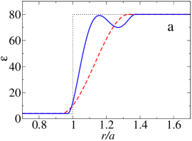
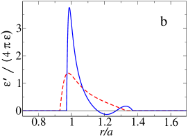
Figure 1: Radial dependence of (a) the dielectric constant $\epsilon(r/a)$ and (b) $\epsilon^{\prime}(r/a)/(4\pi\epsilon(r/a))$ for a monotonic step (red broken line, Eq. (68)) and for a non-monotonic step simulating a hydration layer (blue solid line). The dielectric constant changes smoothly from $\epsilon_{1}=4$ inside the sphere to ${\epsilon_{\rm o}}=80$ outside. The effective radii $r_{0}=1.13a$ and $r_{0}=1.17a$, respectively, are chosen so that the Born solvation energy in each case is equal to that in the case of a sharp boundary at radius $a$ (shown with dotted line). The half-width of the steps $\delta r=0.2a$.

Let there be point charges $q_{1}$ and $q_{2}$ at the centers of spheres 1 and 2, respectively. The induced charge density is found for rigid spheres as the self-consistent solution of (67) for $\rho_{1}({\tilde{r}}_{1})$ and $\rho_{2}({\tilde{r}}_{2})$. Of course, (67) simplifies dramatically in the case of two spheres and two free charges. For fuzzy spheres, one has to use a continuous version of (67) in which summation over $n$ in (66) is carried out numerically with the $n^{\rm th}$-order terms (65) calculated recursively via numerical integration, analogously to the method for a point charge outside a sphere, see (38), (42) and (44). Notice that the $l=0$ components of the induced densities can only be produced by the free charge inside the corresponding sphere. Notice also that the free charges in the centers of the spheres induce only $l=0$, i.e. spherically-symmetric, components. For these reasons it is convenient to distinguish the $l=0$ and $l\neq 0$ components of the induced charge density.

In accordance with (8), the total energy of the system consists of the following terms:

(i) interaction between the point charges (screened by $\epsilon_{1}$),

$$\frac{q_{1}q_{2}}{\epsilon_{1}L},$$ (69)

where $L$ is the length of the vector ${\rm\bf L}_{1\to 2}=-{\rm\bf L}_{2\to 1}$, connecting the centers of the two spheres,

(iia) interaction between each point charge and the $l=0$ component of the induced charge in the interface region of the other sphere,

$$\frac{1}{2}\left(q_{1}\int\frac{\left.\rho_{2}({\tilde{\rm\bf r}}_{2})\right|_{l=0}}{|{\tilde{\rm\bf r}}_{2}+{\rm\bf L}_{1\to 2}|}\,d{\tilde{\rm\bf r}}_{2}+q_{2}\int\frac{\left.\rho_{1}({\tilde{\rm\bf r}}_{1})\right|_{l=0}}{|{\tilde{\rm\bf r}}_{1}+{\rm\bf L}_{2\to 1}|}\,d{\tilde{\rm\bf r}}_{1}\right),$$ (70)

(iib) interaction between each point charge and the $l\neq 0$ components of the induced charge in the interface region of the other sphere,

$$\frac{1}{2}\left(q_{1}\int\frac{\left.\rho_{2}({\tilde{\rm\bf r}}_{2})\right|_{l\neq 0}}{|{\tilde{\rm\bf r}}_{2}+{\rm\bf L}_{1\to 2}|}\,d{\tilde{\rm\bf r}}_{2}+q_{2}\int\frac{\left.\rho_{1}({\tilde{\rm\bf r}}_{1})\right|_{l\neq 0}}{|{\tilde{\rm\bf r}}_{1}+{\rm\bf L}_{2\to 1}|}\,d{\tilde{\rm\bf r}}_{1}\right),$$ (71)

(iiia) interaction between each point charge and the $l=0$ component of the induced charge in the interface region of the same sphere,

$$\frac{1}{2}\left(q_{1}\int\frac{\left.\rho_{1}({\tilde{\rm\bf r}}_{1})\right|_{l=0}}{{\tilde{r}}_{1}}\,d{\tilde{\rm\bf r}}_{1}+q_{2}\int\frac{\left.\rho_{2}({\tilde{\rm\bf r}}_{2})\right|_{l=0}}{{\tilde{r}}_{2}}\,d{\tilde{\rm\bf r}}_{2}\right),$$ (72)

(iiib) interaction between each point charge and the $l\neq 0$ components of the induced charge in the interface region of the same sphere,

$$\frac{1}{2}\left(q_{1}\int\frac{\left.\rho_{1}({\tilde{\rm\bf r}}_{1})\right|_{l\neq 0}}{{\tilde{r}}_{1}}\,d{\tilde{\rm\bf r}}_{1}+q_{2}\int\frac{\left.\rho_{2}({\tilde{\rm\bf r}}_{2})\right|_{l\neq 0}}{{\tilde{r}}_{2}}\,d{\tilde{\rm\bf r}}_{2}\right),$$ (73)

The sum of terms (i) and (iia) is equal to the energy of interaction of two point charges in dielectric medium ${\epsilon_{\rm o}}$

$$\frac{q_{1}q_{2}}{{\epsilon_{\rm o}}L}.$$ (74)

This energy is the same for rigid and fuzzy spheres. In contrast, terms (iib) are different for rigid and fuzzy spheres and are the main source of differences in the forces in these two situations. Finally, terms (iiib) are zero for the point charges located at the centers of the spheres, while terms (iiia) are the Born solvation energy in this case.

Born solvation energies are quite different for rigid and fuzzy spheres, since for fuzzy spheres the induced charge density tends to accumulate near the inner boundary of the interface region. Indeed, the operator ${\rm\bf C}$ is proportional to $\epsilon^{\prime}(r)/\epsilon(r)$ and $\epsilon(r_{0}-\delta r)=\epsilon_{1}\ll\epsilon(r_{0}+\delta r)={\epsilon_{\rm o}}$. This asymmetry is present at each order $n$ and is preserved after the summation over $n$. Radial dependences of the $l=0$ components of the induced densities are illustrated in Fig. 2. On the other hand, fuzzy and rigid spheres model the same physical objects, so it is reasonable to assume that whatever profile of the dielectric constant is chosen, the Born solvation energy should remain the same. For this reason, we adjust the effective radius $r_{0}$ for each profile of the dielectric constant so that the Born solvation energy is equal to that of a rigid sphere of unit radius, see Fig. 1.

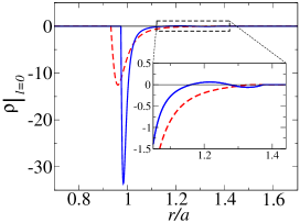
Figure 2: Radial dependence of the induced electric density $\left.\rho(r/a)\right|_{l=0}$ for the monotonic (red broken line) and non-monotonic (blue solid line) steps shown in Fig. 1. The density is normalized by the value of the point charge in the center of the sphere. The inset magnifies a small, oscillatory feature associated with the non-monotonic step.

In Fig. 3 we present the dependence of the interaction energy on distance for a pair of rigid spheres and for two pairs of fuzzy spheres, with monotonic and non-monotonic behaviour of the dielectric function in the interface region, respectively. The energies are normalized to the energy of interaction of point charges (74). The forces between two fuzzy spheres and between two rigid spheres are shown in Fig. 4. The forces are normalized by the interaction force between two point charges. We note that the seemingly weaker effect for the fuzzy spheres with non-monotonic $\epsilon(r)$ dependence is due to the fact that $\epsilon(r)$ changes faster near the inner surface of the interface region to make room for the feature representing the hydration layer. This makes the fuzzy spheres with non-monotonic $\epsilon(r)$ dependence effectively more similar to rigid spheres for fixed $\delta r$ (compare the charge density distributions in Fig. 2).

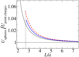
Figure 3: Energy of interaction between two spheres with sharp (thin line) and smeared (thick lines) boundaries. The red broken thick line corresponds to the case of the monotonic radial dependence of the dielectric constant, while the blue solid thick line corresponds to the non-monotonic radial dependence shown in Fig. 1. Free charges of the same sign are located at the centers of the spheres. The energies are normalized by the Coulomb energy of these point charges in the uniform dielectric medium ${\epsilon_{\rm o}}$. The vertical dotted lines indicate the contact points.

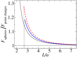
Figure 4: Interaction forces between two spheres with sharp and smeared boundaries. The line identifications are same as in Fig. 3.

For very thin interface regions ($\delta r\to 0$), the forces between two rigid and two fuzzy spheres are equal, as expected. For fuzzy spheres with moderate interface region widths, the repulsion increases with the width. However, this trend quickly saturates (Fig. 5). Qualitatively, this saturation can be explained by two opposing effects. The increase in the interface width increases the size of the spheres thereby strengthening the repulsion. On the other hand, the induced charge density tends to concentrate near the inner surface of the interface which remains around $r=a$ to maintain constant Born solvation energy. Therefore, the bulk of the induced charge on one sphere becomes farther from that of the other sphere, hence weakening the repulsion.

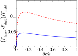
Figure 5: Maximum difference in interaction forces between two spheres with smeared and two spheres with sharp boundaries, occuring at the contact point $2(r_{0}+\delta r)$, as a function of half width of the interface region $\delta r$. The forces are normalized by the interaction force between two spheres with sharp boundaries. The red broken line corresponds to the case of the monotonic radial dependence of the dielectric constant, while the blue solid line corresponds to the non-monotonic radial dependence shown in Fig. 1.

We finally note, that if the point charges are located away from the centers of the spheres, the terms (iiib) depend on the relative position and orientation of the spheres. In this case one can still define the Born solvation energies as the sum of terms (iiia) and (iiib) at large separations, but the terms (iiib) would contribute to the difference of interaction forces/energies between the rigid and fuzzy spheres.

V Conclusions

We have presented an energy minimization formulation of electrostatics that allows computation of the electrostatic energy and forces to any desired accuracy in a system with arbitrary dielectric properties. We have derived an integral equation for the scalar charge density from an energy functional of the polarization vector field. This energy functional represents the true energy of the system even in non-equilibrium states. Arbitrary accuracy is achieved by solving the integral equation for the charge density via a series expansion in terms of the equation’s kernel, which depends only on the geometry of the dielectrics. The streamlined formalism operates with volume charge distributions only, not resorting to introducing surface charges by hand as is done in various other studies of electrostatics via energy minimization. Therefore, it can be applied to arbitrary spatial variations of the dielectric susceptibility. The simplicity of application of the formalism to real problems has been shown with three analytic examples and with a numerical case study. We found that finite boundary widths introduce a measurable correction to the interaction forces as compared to sharp boundary case. For two charged identical spheres the correction is about 10%.

The formalism has various potential applications in modeling electrostatic interactions between solvated molecules: it enables one to go beyond the widely used simplification of atoms and molecules as dielectric balls immersed in a dielectric solvent, as was first suggested by Born in the early twenties of the last century Born . For example, the description of an aqueous solvent as a continuous and homogeneous dielectric medium fails to account for the strong dielectric response of water molecules around charges. Normally, charged ions and surfaces give rise to hydration layers by orienting and displacing surrounding water molecules. These hydration phenomena are very important in many biological processes such as protein folding, protein crystallization, and interactions between charged biopolymers inside the cell. With our formalism one can now consider arbitrary structures for such hydration layers and arrive at a possibly more realistic and reliable analysis of the molecular mechanisms in bio-chemical interactions.

Applied to MD simulations, this formulation is still an implicit solvent scheme, and the position-dependent susceptibility is therefore a model parameter (indeed, the only one). To obtain an estimate of the macroscopic dielectric susceptibility at the molecular level or at the intermolecular boundaries one has to explore physics at the atomic level and introduce some coarse graining. Given that the dielectric susceptibility is related to the charge fluctuations as a response to external perturbations, one can estimate susceptibilites through the study of linear/nonlinear response. For example, the dielectric susceptibility can be related to the correlations of the net system dipole moment and local polarization density Stern . A fully quantum mechanical treatment of solvation of biological systems might be hindered by limits of numerical accuracy Kohn.Nobel and will demand much more computational power than currently available. We believe that quantum mechanics, in particular, density functional theory, can in principle be used to calculate the local dielectric susceptibility which in turn should be used as input for the implicit solvent methods, such as the one described in this paper.

Appendix A Sharp boundary limit in the planar interface problem

Let us demonstrate how a rigorous limiting procedure applied to (25) produces correct expression for the surface charge density in the case of sharp planar interface. The surface charge is found by integrating the charge density over the range $-a\leq z\leq a$ in which $\chi$ changes from ${\chi_{2}}$ to ${\chi_{1}}$, and then taking the limit $a\rightarrow 0$.

We return to (24) and, making use of the azimuthal symmetry of the problem, expand the kernels in terms of Bessel functions $J_{m}$ Jackson ,

$$\frac{1}{|{\rm\bf r}-{\rm\bf r}^{\prime}|} = \sum_{m=-\infty}^{\infty}\int_{0}^{\infty}e^{i\,m(\phi-\phi^{\prime})}\,J_{m}(k\rho)\,J_{m}(k\rho^{\prime})e^{-k(z_{>}-z_{<})}dk$$ (75)

$$\frac{1}{|{\rm\bf r}-d\,\hat{z}|} = \int_{0}^{\infty}J_{0}(k\rho)e^{-k(d-z)}dk.$$ (76)

Here the position vectors ${\rm\bf r}$ and ${\rm\bf r}^{\prime}$ are represented via the polar vectors $\boldsymbol{\rho}$ and $\boldsymbol{\rho}^{\prime}$ in the $z=0$ plane, ${\rm\bf r}=\boldsymbol{\rho}+z\hat{z}$ and ${\rm\bf r}^{\prime}=\boldsymbol{\rho}^{\prime}+z^{\prime}\hat{z}$. The polar vectors are in turn defined through their lengths $\rho=\sqrt{x^{2}+y^{2}}$ and $\rho^{\prime}=\sqrt{x^{\prime 2}+y^{\prime 2}}$ and their azimuthal angles $\phi$ and $\phi^{\prime}$. The notation $z_{>}$ ($z_{<}$) is used for the greater (lesser) of the corresponding $z$ and $z^{\prime}$.

We now treat each of the terms in the expansion of (24) separately. The first term is the screened point charge. All other terms form the induced charge density at the interfacial region. The first contribution to the induced charge density is given by

$${\rho_{\rm i}}^{(1)}({\rm\bf r})=-\frac{q}{\epsilon_{1}}\frac{\epsilon^{\prime}(z)}{4\pi\epsilon(z)}\frac{z-d}{|{\rm\bf r}-d\,\hat{z}|^{3}}.$$ (77)

The corresponding surface charge density is

$${\sigma_{\rm i}}^{(1)}(\boldsymbol{\rho})=-\frac{q}{\epsilon_{1}}\lim_{a\rightarrow 0}\int_{-a}^{a}\frac{\epsilon^{\prime}(z)}{4\pi\epsilon(z)}\left[\frac{-d}{|\boldsymbol{\rho}-d\,\hat{z}|^{3}}+{\cal O}(z)\right]dz.$$ (78)

All the ${\cal O}(z)$ terms vanish since for any bounded function $h(z)$

$$\lim_{a\rightarrow 0}\int_{-a}^{a}z^{n}h(z)dz\leq\lim_{a\rightarrow 0}a^{n}\int_{-a}^{a}|h(z)|dz=0,\;\;\;\;\forall\;\;n>0.$$ (79)

Thus,

$${\sigma_{\rm i}}^{(1)}(\boldsymbol{\rho})=\frac{q}{4\pi\epsilon_{1}}\frac{d}{|\boldsymbol{\rho}-d\,\hat{z}|^{3}}(f_{1}-f_{2}).$$ (80)

Here we have used the notations $f(z)=\ln[\epsilon(z)]$, $f_{1}=f(a)=\ln[\epsilon_{1}]$ and $f_{2}=f(-a)=\ln[\epsilon_{2}]$.

We can similarly evaluate all the other contributions to the induced surface charge density. The second contribution to the induced charge density is

$${\rho_{\rm i}}^{(2)}({\rm\bf r})=\frac{q}{\epsilon_{1}}\frac{\epsilon^{\prime}(z)}{4\pi\epsilon(z)}\int\frac{z-z^{\prime}}{|{\rm\bf r}-{\rm\bf r}^{\prime}|^{3}}\frac{\epsilon^{\prime}(z^{\prime})}{4\pi\epsilon(z^{\prime})}\frac{z^{\prime}-d}{|{\rm\bf r}^{\prime}-d\,\hat{z}|^{3}}\rho^{\prime}d\rho^{\prime}d\phi^{\prime}dz^{\prime}$$ (81)

Using (75), (76), and the completeness relation for Bessel functions Jackson ,

$$\int_{0}^{\infty}J_{m}(k\rho)J_{m}(k^{\prime}\rho)\rho d\rho=\frac{1}{k}\delta(k-k^{\prime}),$$ (82)

we obtain, after integration over $\phi^{\prime}$ and $\rho^{\prime}$,

$${\rho_{\rm i}}^{(2)}({\rm\bf r}) = \frac{q}{\epsilon_{1}}\frac{\epsilon^{\prime}(z)}{4\pi\epsilon(z)}\frac{d}{dz}\int\frac{\epsilon^{\prime}(z^{\prime})}{4\pi\epsilon(z^{\prime})}\int_{0}^{\infty}J_{0}(k\rho)e^{-k(d-z^{\prime})}e^{-k(z_{>}-z_{<})}2\pi dkdz^{\prime}$$ (83)

$$= \frac{q}{\epsilon_{1}}\frac{\epsilon^{\prime}(z)}{4\pi\epsilon(z)}\frac{1}{2}\int_{0}^{\infty}kdke^{-k(d-z)}J_{0}(k\rho)\times$$

$$\hskip 72.26999pt\left[\int_{z}^{a}\frac{\epsilon^{\prime}(z^{\prime})}{\epsilon(z^{\prime})}dz^{\prime}-\int_{-a}^{z}\frac{\epsilon^{\prime}(z^{\prime})}{\epsilon(z^{\prime})}e^{-2k(z-z^{\prime})}dz^{\prime}\right].$$

The corresponding surface charge density is then

$${\sigma_{\rm i}}^{(2)} = \frac{q}{\epsilon_{1}}\lim_{a\rightarrow 0}\int_{-a}^{a}dz\frac{\epsilon^{\prime}(z)}{4\pi\epsilon(z)}\frac{1}{2}\int_{0}^{\infty}kdke^{-k(d-z)}J_{0}(k\rho)\times$$ (84)

$$\hskip 72.26999pt\left[\int_{z}^{a}\frac{\epsilon^{\prime}(z^{\prime})}{\epsilon(z^{\prime})}dz^{\prime}-\int_{-a}^{z}\frac{\epsilon^{\prime}(z^{\prime})}{\epsilon(z^{\prime})}e^{-2k(z-z^{\prime})}dz^{\prime}\right].$$

Applying to (84) the same argument used in deriving (80),

$${\sigma_{\rm i}}^{(2)}=\frac{q}{\epsilon_{1}}\int_{0}^{\infty}kdke^{-kd}J_{0}(k\rho)\lim_{a\rightarrow 0}\int_{-a}^{a}dz\frac{\epsilon^{\prime}(z)}{4\pi\epsilon(z)}\frac{1}{2}\left[\int_{z}^{a}\frac{\epsilon^{\prime}(z^{\prime})}{\epsilon(z^{\prime})}dz^{\prime}-\int_{-a}^{z}\frac{\epsilon^{\prime}(z^{\prime})}{\epsilon(z^{\prime})}dz^{\prime}\right].$$ (85)

The integral over $k$ is evaluated using (76) as

$$\int kJ_{0}(k\rho)e^{-kd}dk=\left.\frac{d}{dz}\int J_{0}(k\rho)e^{-k(d-z)}dk\right|_{z=0}=\left.\frac{d}{dz}\frac{1}{|{\rm\bf r}-d\,\hat{z}|}\right|_{z=0}=\frac{d}{|\boldsymbol{\rho}-d\,\hat{z}|^{3}}.$$ (86)

Then

$${\sigma_{\rm i}}^{(2)}=\frac{q}{\epsilon_{1}}\frac{d}{|\boldsymbol{\rho}-d\,\hat{z}|^{3}}\lim_{a\rightarrow 0}\int_{-a}^{a}dz\frac{\epsilon^{\prime}(z)}{4\pi\epsilon(z)}\left[\frac{1}{2}(f_{1}+f_{2})-f(z)\right].$$ (87)

Finally, we obtain that ${\sigma_{\rm i}}^{(2)}=0$,

$${\sigma_{\rm i}}^{(2)}=\frac{q}{4\pi\epsilon_{1}}\frac{d}{|\boldsymbol{\rho}-d\,\hat{z}|^{3}}\int_{f_{2}}^{f_{1}}df\left[\frac{1}{2}(f_{1}+f_{2})-f(z)\right]=0.$$ (88)

Analogously, the expressions for the induced surface charge densities up to the fifth order are found to be

$${\sigma_{\rm i}}^{(1)} = \frac{q}{4\pi\epsilon_{1}}\frac{d}{|\boldsymbol{\rho}-d\,\hat{z}|^{3}}(f_{1}-f_{2}),$$

$${\sigma_{\rm i}}^{(2)} = 0,$$

$${\sigma_{\rm i}}^{(3)} = \frac{q}{4\pi\epsilon_{1}}\frac{d}{|\boldsymbol{\rho}-d\,\hat{z}|^{3}}\frac{-1}{12}(f_{1}-f_{2})^{3},$$

$${\sigma_{\rm i}}^{(4)} = 0,$$

$${\sigma_{\rm i}}^{(5)} = \frac{q}{4\pi\epsilon_{1}}\frac{d}{|\boldsymbol{\rho}-d\,\hat{z}|^{3}}\frac{1}{120}(f_{1}-f_{2})^{5}.$$ (89)

In general, the surface charge density is of the form

$${\sigma_{\rm i}}^{(n)}(z) = -\frac{q}{\epsilon_{1}}\lim_{a\rightarrow 0}\int_{-a}^{a}dz\frac{\epsilon^{\prime}(z)}{4\pi\epsilon(z)}\frac{z-d}{|{\rm\bf r}-d\,\hat{z}|^{3}}\times$$ (90)

$$\qquad\frac{1}{2}\left[\int_{z}^{a}\frac{\epsilon^{\prime}(z^{\prime})}{\epsilon(z^{\prime})}g^{(n-1)}(f(z^{\prime}))dz^{\prime}-\int_{-a}^{z}\frac{\epsilon^{\prime}(z^{\prime})}{\epsilon(z^{\prime})}g^{(n-1)}(f(z^{\prime}))dz^{\prime}\right]$$

$$= -\frac{q}{\epsilon_{1}}\lim_{a\rightarrow 0}\frac{1}{2}\int_{-a}^{a}dz\frac{\epsilon^{\prime}(z)}{4\pi\epsilon(z)}\frac{z-d}{|{\rm\bf r}-d\,\hat{z}|^{3}}g^{(n)}(f(z))$$

$$= \frac{q}{4\pi\epsilon_{1}}\frac{d}{|\boldsymbol{\rho}-d\,\hat{z}|^{3}}\int_{f_{2}}^{f_{1}}g^{(n)}(f)df.$$

The functions $g^{(n)}(f(z))$ up to $n=5$ are

$$g^{(1)}(f(z)) = 1$$

$$g^{(2)}(f(z)) = -f(z)+\frac{1}{2}(f_{1}+f_{2})$$

$$g^{(3)}(f(z)) = \frac{f^{2}(z)}{2}-\frac{1}{2}(f_{1}+f_{2})\,f(z)+\frac{1}{2}f_{1}f_{2}$$

$$g^{(4)}(f(z)) = -\frac{f^{3}(z)}{6}+\frac{1}{4}(f_{1}+f_{2})\,f^{2}(z)-\frac{1}{2}f_{1}f_{2}f(z)-\frac{1}{24}(f_{1}+f_{2})(f_{1}^{2}-4f_{1}f_{2}+f_{2}^{2})$$

$$g^{(5)}(f(z)) = \frac{f^{4}(z)}{24}-\frac{1}{12}(f_{1}+f_{2})\,f^{3}(z)+\frac{1}{4}f_{1}f_{2}f^{2}(z)+\frac{1}{24}(f_{1}+f_{2})(f_{1}^{2}-4f_{1}f_{2}+f_{2}^{2})f(z)$$ (91)

$$\hskip 72.26999pt-\frac{1}{24}f_{1}f_{2}(f_{1}^{2}-3f_{1}f_{2}+f_{2}^{2}).$$

We will show by induction that $g^{(n)}(f)$ is

$$g^{(n)}(f) = (-1)^{n-1}\frac{1}{(n-1)!}f^{n-1}+\frac{1}{2}\left[C_{1}\,g^{(n-1)}(f)-\frac{1}{2!}C_{2}\,g^{(n-2)}(f)+\frac{1}{3!}C_{3}\,g^{(n-3)}(f)+\cdots\right.$$ (92)

$$\hskip 108.405pt\left.+(-1)^{n-2}\frac{1}{(n-1)!}C_{n-1}\,g^{(1)}(f)\right]$$

$$= \frac{(-1)^{n-1}f^{n-1}}{(n-1)!}+\frac{1}{2}\sum_{m=1}^{n-1}\frac{(-1)^{n-m-1}C_{n-m}}{(n-m)!}g^{(m)}(f),$$

where the coefficients $C_{n}=f_{1}^{n}+f_{2}^{n}$. First, (92) can be explicitly verified up to $n=5$ using (91). Second, we show that if this expression holds for some integer $n$, then it also holds for $n+1$. From Eq.(90) we can write,

$$g^{(n+1)}(f(z)) = \frac{1}{2}\left[\int_{f(z)}^{f_{1}}g^{(n)}(f)df-\int_{f_{2}}^{f(z)}g^{(n)}(f)df\right]$$ (93)

$$= \frac{(-1)^{n-1}}{(n-1)!}\frac{1}{2}\left[\int_{f(z)}^{f_{1}}f^{n-1}df-\int_{f_{2}}^{f(z)}f^{n-1}df\right]$$

$$\hskip 36.135pt+\frac{1}{2}\sum_{m=1}^{n-1}\frac{(-1)^{n-m-1}C_{n-m}}{(n-m)!}\frac{1}{2}\left[\int_{f(z)}^{f_{1}}g^{(m)}(f)df-\int_{f_{2}}^{f(z)}g^{(m)}(f)df\right]$$

$$= \frac{(-1)^{n}f^{n}}{n!}+\frac{1}{2}\frac{(-1)^{n-1}(f_{1}^{n}+f_{2}^{n})}{n!}+\frac{1}{2}\sum_{m=1}^{n-1}\frac{(-1)^{n-m-1}C_{n-m}}{(n-m)!}g^{(m+1)}(f)$$

$$= \frac{(-1)^{(n+1)-1}f^{(n+1)-1}}{((n+1)-1)!}+\frac{1}{2}\sum_{m=1}^{(n+1)-1}\frac{(-1)^{(n+1)-m-1}C_{(n+1)-m}}{((n+1)-m)!}g^{(m)}(f)$$

We thus proved that $g^{(n)}(f)$ is given by (92) for any given integer $n\geq 2$ with $g^{(1)}(f)=1$.

We now need to find the integral $\int{\sigma_{\rm i}}^{(n)}$ in (90). We will show by induction that

$$\int_{f_{2}}^{f_{1}}g^{(n)}(f)=-2\frac{E_{n}}{n!}u^{n},$$ (94)

where $u=f_{1}-f_{2}$ and $E_{n}$ are the coefficients of the expansion

$$\frac{2}{e^{u}+1}=\sum_{n=0}^{\infty}\frac{E_{n}}{n!}u^{n}.$$ (95)

It is easy to see that $E_{0}=1$.

The base for the mathematical induction for (94) is easily established for the first few terms using (91). Now we verify that (94) holds true for $n+1$ if it is true for $n$. To do so, we integrate both sides of (93) and use the assumption (94) to obtain

$$\int_{f_{2}}^{f_{1}}g^{(n+1)}(f) = -\frac{(-1)^{(n+1)}}{(n+1)!}(f_{1}^{n+1}-f_{2}^{n+1})+\sum_{m=1}^{n}\frac{(-1)^{n+1-m}}{(n+1-m)!m!}C_{n+1-m}E_{m}u^{m}$$ (96)

$$=-2\frac{(-f_{1})^{n+1}}{(n+1)!}+\sum_{m=0}^{n}\frac{(-f_{1})^{n+1-m}}{(n+1-m)!}\frac{E_{m}u^{m}}{m!}+\sum_{m=0}^{n}\frac{(-f_{2})^{n+1-m}}{(n+1-m)!}\frac{E_{m}u^{m}}{m!}$$

$$=-2\frac{(-f_{1})^{n+1}}{(n+1)!}+\sum_{m=0}^{n+1}\left[\frac{(-f_{1})^{n+1-m}}{(n+1-m)!}+\frac{(-f_{2})^{n+1-m}}{(n+1-m)!}\right]\frac{E_{m}u^{m}}{m!}-2\frac{E_{n+1}u^{n+1}}{(n+1)!}.$$

In the second step we have included an $m=0$ term in the summation and in the third step we have added and subtracted an $m=n+1$ term. It can be easily verified that the right hand side of (96) is the $s^{n+1}$ term of the following expression.

$$-2e^{-f_{1}s}+\left[e^{-f_{1}s}+e^{-f_{2}s}-2\right]\frac{2}{e^{us}+1}=-2\frac{2}{e^{us}+1}\\ =-2\sum_{m=0}^{\infty}\frac{E_{m}u^{m}}{m!}s^{m}.$$

This completes the proof.

Summing over all the terms, we have

$$\sum_{n=1}^{\infty}\int_{f_{2}}^{f_{1}}g^{(n)}(f)=-2\sum_{n=0}^{\infty}\frac{E_{n}u^{n}}{n!}+2E_{0}=2\left(1-\frac{2}{e^{u}+1}\right)=\frac{2(\epsilon_{1}-\epsilon_{2})}{\epsilon_{1}+\epsilon_{2}}$$ (97)

We note that the series converges for $|u|={\rm ln}{\epsilon_{\rm o}}/\epsilon_{1}<\pi$. This means that if one medium is water (${\epsilon_{\rm o}}\approx 80$) then for the other material the dielectric constant $\epsilon_{1}>{\epsilon_{\rm o}}e^{-\pi}\approx 3.47$. However, using techniques similar to Borel summation, one can show that the series can still be summed to the correct final formula for larger values of $|u|$.

Finally the induced surface charge density becomes

$${\sigma_{\rm i}}(\boldsymbol{\rho})=\frac{q}{4\pi\epsilon_{1}}\frac{2(\epsilon_{1}-\epsilon_{2})}{\epsilon_{1}+\epsilon_{2}}\frac{d}{|\boldsymbol{\rho}-d\,\hat{z}|^{3}},$$ (98)

which is identical to (27). Thus, we have rigorously justified using the average dielectric constant $(\epsilon_{1}+\epsilon_{2})/2$ at the boundary.

Appendix B Evaluation of $\Lambda$ for Spheres with Sharp Boundaries

To compute $\Lambda^{j}_{lm}(a_{j},{\rm\bf L}_{j\to k})$, defined as

$$\Lambda^{j}_{lm}(a_{j},{\rm\bf L}_{j\to k})\equiv\int{Y_{lm}^{*}({{\tilde{\rm\bf r}}_{j}-{\rm\bf L}_{j\to k}\over|{\tilde{\rm\bf r}}_{j}-{\rm\bf L}_{j\to k}|})\over|{\tilde{\rm\bf r}}_{j}-{\rm\bf L}_{j\to k}|^{l+1}}\rho_{j}({\tilde{\rm\bf r}}_{j})d{\tilde{\rm\bf r}}_{j}\;,$$ (99)

for the case of spheres with sharp boundaries, expand the charge density on sphere $j$ as

$$\rho_{j}({\tilde{\rm\bf r}}_{j})=\delta({\tilde{r}}_{j}-a_{j})\sum_{l^{\prime},m^{\prime}}\sqrt{4\pi}\sigma^{j}_{l^{\prime}m^{\prime}}Y_{l^{\prime}m^{\prime}}({\hat{\tilde{r}}}_{j})$$ (100)

to find

$$\Lambda^{j}_{lm}(a_{j},{\rm\bf L}_{j\to k})=\sum_{l^{\prime},m^{\prime}}\sqrt{4\pi}\sigma^{j}_{l^{\prime}m^{\prime}}\int{Y_{lm}^{*}({{\tilde{\rm\bf r}}_{j}-{\rm\bf L}_{j\to k}\over|{\tilde{\rm\bf r}}_{j}-{\rm\bf L}_{j\to k}|})Y_{l^{\prime}m^{\prime}}({\hat{\tilde{r}}}_{j})\over L_{j\to k}^{l+1}(1+t^{2}-2t\cos{\tilde{\theta}}_{j})^{(l+1)/2}}\delta({\tilde{r}}_{j}-a_{j})d{\tilde{\rm\bf r}}_{j}\;,$$ (101)

where use has been made of the geometrical fact that $|{\tilde{\rm\bf r}}_{j}-{\rm\bf L}_{j\to k}|=L_{j\to k}\sqrt{1+t^{2}-2t\cos{\tilde{\theta}}_{j}}$ with $t\equiv{\tilde{r}}_{j}/L_{j\to k}$. The delta function renders the radial integration trivial:

$$\Lambda^{j}_{lm}(a_{j},{\rm\bf L}_{j\to k})=\sum_{l^{\prime},m^{\prime}}\sqrt{4\pi}a_{j}^{2}\sigma^{j}_{l^{\prime}m^{\prime}}\int{Y_{lm}^{*}(\vartheta,\varphi)Y_{l^{\prime}m^{\prime}}({\tilde{\theta}}_{j},{\tilde{\phi}}_{j})\over L_{j\to k}^{l+1}(1+t^{2}-2t\cos{\tilde{\theta}}_{j})^{(l+1)/2}}d(\cos{\tilde{\theta}}_{j})d{\tilde{\phi}}_{j}\;,$$ (102)

where $\vartheta$ and $\varphi$ are the polar variables of $({\tilde{\rm\bf r}}_{j}-{\rm\bf L}_{j\to k})/|{\tilde{\rm\bf r}}_{j}-{\rm\bf L}_{j\to k}|$ and $t=a_{j}/L_{j\to k}$ now. All of the angular variables are measured with respect to a coordinate system whose $z$ axis is parallel to ${\rm\bf L}_{j\to k}$. The angles $\vartheta$ and $\varphi$ must be expressed as functions of the integration variables ${\tilde{\theta}}_{j}$ and ${\tilde{\phi}}_{j}$:

$$\cos\vartheta = (t\cos{\tilde{\theta}}_{j}-1)\over\sqrt{1+t^{2}-2t\cos{\tilde{\theta}}_{j}}$$ (103)

$$\varphi = {\tilde{\phi}}_{j}\;.$$ (104)

Since the definition of the spherical harmonics is

$$Y_{lm}(\theta,\phi)=\sqrt{\frac{(2l+1)(l-m)!}{4\pi(l+m)!}}P_{lm}(\cos\theta)e^{im\phi}\;,$$ (105)

$\Lambda$ is

$$\Lambda^{j}_{lm}(a_{j},{\rm\bf L}_{j\to k}) = \sum_{l^{\prime},m^{\prime}}\frac{\sqrt{4\pi}a_{j}^{2}\sigma^{j}_{l^{\prime}m^{\prime}}}{L_{j\to k}^{l+1}}\left[\frac{(2l+1)(l-m)!(2l^{\prime}+1)(l^{\prime}-m^{\prime})!}{4\pi(l+m)!4\pi(l^{\prime}+m^{\prime})!}\right]^{1/2}$$ (106)

$$\times \int\frac{P_{lm}(\frac{(t\cos{\tilde{\theta}}_{j}-1)}{\sqrt{1+t^{2}-2t\cos{\tilde{\theta}}_{j}}})P_{l^{\prime}m^{\prime}}(\cos{\tilde{\theta}}_{j})}{(1+t^{2}-2t\cos{\tilde{\theta}}_{j})^{(l+1)/2}}d(\cos{\tilde{\theta}}_{j})d{\tilde{\phi}}_{j}\;.$$ (107)

The integration over ${\tilde{\phi}}_{j}$ produces $2\pi\delta_{mm^{\prime}}$. The integration over $\cos{\tilde{\theta}}_{j}$ is then the integral calcuated by YuYu . The final expression for $\Lambda$ is

$$\Lambda^{j}_{lm}(a_{j},{\rm\bf L}_{j\to k})=\sum_{l^{\prime}}\frac{Q^{j}_{l^{\prime}m}t^{l^{\prime}}(-1)^{l-m}(l+l^{\prime})!\sqrt{2l+1}}{L_{j\to k}^{l+1}[4\pi(l+m)!(l^{\prime}+m)!(l-m)!(l^{\prime}-m)!(2l^{\prime}+1)]^{1/2}}\;,$$ (108)

where $Q^{j}_{l^{\prime}m}\equiv 4\pi a_{j}^{2}\sigma^{j}_{l^{\prime}m}$.

References

• (1) A. Wallqvist and R. D. Mountain, Reviews in Computational Chemistry 13, 183 (1999).
• (2) W. L. Jorgensen and J. Tirado-Rives, Proc. Natl. Acad. Sci. U.S.A. 102, 6665 (2005).
• (3) B. Guillot, J. Mol. Liq. 101, 219 (2002).
• (4) J. Chen, C. L. Brooks III, J. Khandogin, Current Opinion in Structural Biology 18, 140 (2008).
• (5) B. H. Honig, W. L. Hubbell and R. F. Flewelling, Annu. Rev. Biophys. Biophys. Chem. 15, 163 (1986).
• (6) J. Tomasi and M. Persico, Chem. Rev. 94, 2027 (1994).
• (7) C. J. Cramer and D. G. Truhlar, Chem. Rev. 99, 2161 (1999).
• (8) D. Bashford and D. A. Case, Annu. Rev. Phys. Chem. 51, 129 (2000).
• (9) T. P. Doerr and Y.-K. Yu, Phys. Rev. E 373, 061902 (2006).
• (10) B. Bagchi, Chem. Rev. 105, 3197 (2005).
• (11) J. Schwinger, L. L. Deraad, K. A. Milton, W. Tsai and J. Norton, Classical Electrodynamics (Westview Press, 1998).
• (12) J. D. Jackson, Classical Electrodynamics 3rd Edn., Chapter 1, page 43, (John Wiley & Sons, Inc. 1999).
• (13) J. Che, J. Dzubiella, B. Li, and J. A. McCammon, J. Phys. Chem. B 112, 3058 (2008).
• (14) R. Allen, J-P Hansen and S. Melchionna, Phys. Chem. Chem. Phys. 3, 4177 (2001).
• (15) R. A. Marcus, J. Chem. Phys. 24, 979 (1956); ibid 24, 966 (1956).
• (16) B. U. Felderhof, J. Chem. Phys. 67, 493 (1977).
• (17) M. Marchi, D. Borgis, N. Levy and P. Ballone, J. Chem. Phys. 114, 4377 (2001). We believe that the citation supporting Eq. (2) (the energy functional) in this paper should only invoke Felderhof’s paper Felderhof (and not Marcus’s). N. Levy, D. Borgis and M. Marchi, Comp. Phys. Comm., 169, 69 (2005).
• (18) P. Attard, J. Chem. Phys. 119, 1365 (2003).
• (19) R. P. Feynman, R. B. Leighton and M. Sands, The Feynman Lectures on Physics II, Chapter 10, pages 10-2 (Addison-Wesley, 1964).
• (20) L. D. Landau, E. M. Lifschits, The course of theoretecal physics. Volume VIII: The electrodynamics of continuous media, 2 edition (Butterworth-Heinemann, 1984)
• (21) F. Fogolari and J. M. Briggs, Chem. Phys. Lett. 281, 135 (1997).
• (22) D. H. Menzel, Fundamental Formulas of Physics, (New York: Prentice-Hall, 1955)
• (23) Y.-K. Yu, Physica A 326, 522 (2003).
• (24) M. Born, Z. Phys. 1, 45 (1920).
• (25) H. A. Stern and S. E. Feller, J. Chem. Phys. 118, 3401 (2003).
• (26) W. Kohn, Reviews of Modern Physics 71, 1253 (1999).