Exact solutions of an $SO(5)$-invariant spin-$3/2$ Fermi gas model

Abstract

An exactly solvable model describing the dilute spin-$3/2$ fermion gas in one-dimensional optical trap is proposed. The diagonalization of the model Hamiltonian is derived by means of the Bethe ansatz method. Exotic spin excitations such as the heavy spinon with fractional spin $3/2$, the neutral spinon with spin zero and the dressed spinon with spin $1/2$ are found based on the exact solution.

The study on the optically and magnetically trapped ultracold atoms has attracted a lot of attentions in the recent years. By using the magnetic fields or laser beams, the atoms can be trapped and cooled down to very low temperatures MGreiner01 ; AGolitz01 ; FSchreck01 ; HMoritz03 ; h ; b1 ; TKinoshita04 ; BParedes04 ; HMoritz05 ; SAubin05 . A fascinating fact is that not only the components but also the physical parameters of such systems can be manipulated in experiments, which allow us to mimic the ordinary correlated electron systems and even to explore new states of matter. For examples, by means of the Feshbach resonance techniques, one can tune the scattering lengths or the interactions among the atoms; putting an optical lattice on one can study the behaviors of the atoms in a tunable periodic potential and with strong anisotropic traps, the one- and two-dimensional quantum systems can be realized. One of the hot research topics in this field is the study on the high spin cold atom systems. The physics of bosonic ultracold atoms with hyperfine spin $F=1$ have been extensively studied sbec2 ; sbec3 ; mfpt1 ; e1 ; e2 ; cao . The degenerate Fermi gas with hyperfine spin $F=3/2$ could be obtained by cooling alkali atoms ¹³²Cs, as well as alkaline-earth atoms ⁹Be, ¹³⁵Ba and ¹³⁷Ba in experiments. The ground states of these high spin fermionic atoms in optical traps are very rich. Many peculiar quantum orders and exotic collective excitations appear in these systems, which are rare in the ordinary interacting electron systems 10 . Several methods have been developed to approach these ultracold atom systems. For examples, Wu et al. showed that the one-dimensional (1D) spin-$3/2$ Fermi gas with s-wave scattering possesses the $SO(5)$-invariance and obtained the phase diagram of the system by means of bosonization wu1 ; wu3 ; the functional integral approach was applied on the interacting spin-$3/2$ fermionic ultracold atoms in 2D square optical lattice to study a variety of Mott insulating phases zhang1 ; zhang2 ; two different superfluid phases in $F=N-1/2$ fermionic cold atom system were found, i.e., an unconfined BCS pairing phase and a confined molecular-superfluid made of $2N$ fermions, depending on whether a discrete symmetry is spontaneously broken or not p .

Despite the fast progress in this field, the understanding to the high-spin correlated systems is still far from satisfied. Reference models with exact solutions are undoubtedly needed to get deep insight about these interesting quantum many-body systems. An important progress in this aspect is made by Controzzi1 and Tsvelik, who constructed an exactly solvable model for isospin $F=3/2$ fermionic system with linear dispersion relations c . In this Letter, we propose a new exactly solvable model which describes properly a 1D spin-$3/2$ cold atom system. With the Bethe ansatz solutions, we derive out exactly the ground state. Exotic spin excitations such as the heavy spinons with fractional spin $3/2$, the neutral spinons with zero spin and the dressed spinons with spin $1/2$ are found.

The fermions with hyperfine spin $F=3/2$ in a 1D trap is appropriately described by the following model Hamiltonian

$$H=\sum_{j=1}^{N}\left[-\frac{\partial^{2}}{\partial x_{j}^{2}}+V_{e}(x_{j})\right]+\sum_{l<j,m}^{N}g_{m}\delta(x_{j}-x_{l})P^{m}_{jl},$$ (1)

where $V_{e}(x_{j})$ is the external potential, $g_{m}$ is the two-body coupling constant in the total spin $m=0,2$ channel and $P_{jl}^{m}$ is the projection operator onto the spin $m$ channel. Because of the antisymmetric wave functions of the fermions, non-trivial scattering processes occur only in the $m=0$ and $m=2$ channels, and those in the $m=1$ and $m=3$ channels are irrelevant for the $\delta$-function interaction potential. In the low density case, we omit the external field. The Hamiltonian (1) can be rewritten as

$$H=-\sum_{j=1}^{N}\frac{\partial^{2}}{\partial x_{j}^{2}}+\sum_{l<j}^{N}(c_{0}+c_{2}{\bf S}_{j}\cdot{\bf S}_{l})\delta(x_{j}-x_{l}),$$ (2)

where $c_{0}=g_{0}/3+2g_{2}/3$, $c_{2}=g_{2}/3-g_{0}/3$ and ${\bf S}_{j}$ is the spin-$3/2$ operator. If $c_{2}=0$, the system (2) is $SU(4)$-invariant and was solved exactly by Sutherland suth . In the present Letter, we show that the system (2) possesses another integrable line $c_{0}=c/2$, $c_{2}=-2c/3$ at which the physical properties are quite different to those of the Sutherland model suth ; sch . An obvious fact is that in our case, the particle number of an individual spin component is no longer conserved because of the broken $SU(4)$-symmetry. Nevertheless, the system (2) is still $SO(5)$-invariant at this new integrable line, and the following three independent conserved quantities are hold:

$$I_{1}=N_{3/2}+N_{1/2}+N_{-1/2}+N_{-3/2},$$

$$I_{2}=N_{3/2}-N_{-3/2},$$ (3)

$$I_{3}=N_{1/2}-N_{-1/2},$$

where $N_{s}$ indicates the particle number with the spin component $s=\pm 1/2,\pm 3/2$.

Assume the wave function takes the following form

$$\Psi(x_{1}s_{1},\cdots,x_{N}s_{N})=\sum_{Q,P}\theta(x_{Q_{1}}<\cdots<x_{Q_{N}})$$

$$\quad\quad\quad\quad\times A_{s_{1}\cdots s_{N}}(Q,P)e^{i\sum_{l=1}^{N}k_{P_{l}}x_{Q_{l}}},$$ (4)

where $Q=(Q_{1},\cdots,Q_{N})$ and $P=(P_{1},\cdots,P_{N})$ are the permutations of the integers $1,\cdots,N$; $k_{j}$ are the quasi momenta carried by the particles; $\theta(x_{Q_{1}}<\cdots<x_{Q_{N}})=\theta(x_{Q_{N}}-x_{Q_{N-1}})\cdots\theta(x_{Q_{2}}-x_{Q_{1}})$ and $\theta(x-y)$ is the step function. With the standard coordinate Bethe ansatz method, we obtain the two-body scattering matrix as

$$S_{jl}=\frac{k_{j}-k_{l}-i\frac{3c}{2}}{k_{j}-k_{l}+i\frac{3c}{2}}P_{jl}^{0}+P_{jl}^{1}+\frac{k_{j}-k_{l}-i\frac{c}{2}}{k_{j}-k_{l}+i\frac{c}{2}}P_{jl}^{2}+P_{jl}^{3},$$ (5)

which satisfies the Yang-Baxter equation

$$S_{12}(k_{1}-k_{2})S_{13}(k_{1}-k_{3})S_{23}(k_{2}-k_{3})$$

$$\quad=S_{23}(k_{2}-k_{3})S_{13}(k_{1}-k_{3})S_{12}(k_{1}-k_{2}).$$ (6)

Applying further the nested algebraic Bethe ansatz with periodic boundary conditions Mar , we obtain the following Bethe ansatz equations(BAE):

$$e^{ik_{j}L}=\prod_{\alpha=1}^{M_{1}}\frac{k_{j}-\lambda_{\alpha}+i\frac{c}{4}}{k_{j}-\lambda_{\alpha}-i\frac{c}{4}},\quad j=1,\cdots,N,$$

$$\prod_{l=1}^{N}\frac{\lambda_{\beta}-k_{l}+i\frac{c}{4}}{\lambda_{\beta}-k_{l}-i\frac{c}{4}}\prod_{\gamma=1}^{M_{2}}\frac{\lambda_{\beta}-\mu_{\gamma}+i\frac{c}{2}}{\lambda_{\beta}-\mu_{\gamma}-i\frac{c}{2}}$$

$$\quad=-\prod_{\alpha=1}^{M_{1}}\frac{\lambda_{\beta}-\lambda_{\alpha}+i\frac{c}{2}}{\lambda_{\beta}-\lambda_{\alpha}-i\frac{c}{2}},\quad\beta=1,\cdots,M_{1},$$ (7)

$$\prod_{\alpha=1}^{M_{1}}\frac{\mu_{\nu}-\lambda_{\alpha}+i\frac{c}{2}}{\mu_{\nu}-\lambda_{\alpha}-i\frac{c}{2}}=-\prod_{\gamma=1}^{M_{2}}\frac{\mu_{\nu}-\mu_{\gamma}+ic}{\mu_{\nu}-\mu_{\gamma}-ic},$$

$$\hskip 119.50148pt\nu=1,\cdots,M_{2},$$

where $N=N_{3/2}+N_{1/2}+N_{-1/2}+N_{-3/2}$, $M_{1}=N_{1/2}+2N_{-3/2}+N_{-1/2}$, $M_{2}=N_{-1/2}+N_{-3/2}$ and $L$ is the length of the system. The corresponding eigen energy of the Hamiltonian is $E=\sum_{j=1}^{N}k_{j}^{2}$.

We consider the $c>0$, i.e., the repulsive interaction case. By carefully checking the structure of the BAE (7), we find that all the charge rapidities $k_{j}$ take real values, indicating the absence of charge bound state. However, the spin rapidities $\lambda_{\beta}$ and $\mu_{\nu}$ may form strings with the following form in the thermodynamic limit

$$\lambda^{n}_{\beta,j}=\lambda^{(n)}_{\beta}+\frac{ic}{4}(n+1-2j),\;j=1,\cdots,n,$$ (8)

$$\mu^{m}_{\nu,j}=\mu^{(m)}_{\nu}+\frac{ic}{2}(n+1-2j),\;j=1,\cdots,m,$$ (9)

where $\lambda^{(n)}_{\beta}$ and $\mu^{(m)}_{\nu}$ are the real parts of the $n$-string of $\lambda$ and the $m$-string of $\mu$, respectively. Denote $\rho$, $\eta_{n}$ and $\sigma_{m}$ as the densities of $k$, $\lambda$ $n$-strings and $\mu$ $m$-strings in the thermodynamic limit $N\to\infty$, $L\to\infty$ and $N/L\to finite$, respectively, and $\rho^{h}$, $\eta_{n}^{h}$ and $\sigma_{m}^{h}$ the corresponding densities of holes. At temperature $T$, the Gibbs free energy of the system with an external magnetic field $h$ and chemical potential $A$ is

$$F=E-AN-h\left(\frac{3}{2}N-M_{1}-M_{2}\right)-TS,$$ (10)

where $E=L\int k^{2}\rho(k)dk$ is the energy; $N=L\int\rho(k)dk$ is the particle number; $M_{1}=L\sum_{n}n\int\eta_{n}(\lambda)d\lambda$; $M_{2}=L\sum_{m}m\int\sigma_{m}(\mu)d\mu$; $S=L\int\{(\rho+\rho^{h})\ln(\rho+\rho^{h})-\rho\ln\rho-\rho^{h}\ln\rho^{h}+\sum_{n}[(\eta_{n}+\eta_{n}^{h})\ln(\eta_{n}+\eta_{n}^{h})-\eta_{n}\ln\eta_{n}-\eta_{n}^{h}\ln\eta_{n}^{h}]+\sum_{m}[(\sigma_{m}+\sigma_{m}^{h})\ln(\sigma_{m}+\sigma_{m}^{h})-\sigma_{m}\ln\sigma_{m}-\sigma_{m}^{h}\ln\sigma_{m}^{h}]\}dk$ denotes the entropy. Minimizing the Gibbs free energy at the thermal equilibrium, we obtain the following thermodynamic Bethe ansatz equations (TBAE)

$$\ln\tilde{\rho}=\frac{k^{2}-A}{T}-\sum_{n}a_{n}*\ln(1+{\tilde{\eta}}_{n}^{-1}),$$

$$\ln{\tilde{\eta}}_{1}=G_{1}*\ln[(1+\tilde{\eta}_{2})(1+\tilde{\rho}^{-1})^{-1}],$$

$$\ln\tilde{\sigma}_{1}=G_{2}*\ln\frac{1+\tilde{\sigma}_{2}}{(1+\tilde{\eta}_{1}^{-1})(1+\tilde{\eta}_{3}^{-1})}$$

$$\quad\quad\quad-\frac{G_{2}}{G_{1}}*\ln(1+\tilde{\eta}_{2}^{-1}),$$

$$\ln\tilde{\eta}_{n\in even}=G_{1}*\ln\frac{(1+\tilde{\eta}_{n-1})(1+\tilde{\eta}_{n+1})}{1+\tilde{\sigma}_{n/2}^{-1}},$$ (11)

$$\ln\tilde{\eta}_{n\in odd}=G_{1}*\ln[(1+\tilde{\eta}_{n-1})(1+\tilde{\eta}_{n+1})],$$

$$\ln\tilde{\sigma}_{m}=G_{2}*\ln\frac{(1+\tilde{\sigma}_{m-1})(1+\tilde{\sigma}_{m+1})}{(1+\tilde{\eta}_{2m-1}^{-1})(1+\tilde{\eta}_{2m+1}^{-1})}$$

$$\quad\quad\quad-\frac{G_{2}}{G_{1}}*\ln(1+\tilde{\eta}_{2m}^{-1}),$$

$$\lim_{n\rightarrow\infty}\frac{\ln\tilde{\eta}_{n}}{n}=\frac{h}{T},\quad\lim_{m\rightarrow\infty}\frac{\ln\tilde{\sigma}_{m}}{m}=\frac{h}{T},$$

where $\tilde{\rho}=\rho_{h}/\rho$, $\tilde{\eta}_{n}=\eta_{n}^{h}/\eta_{n}$, $\tilde{\sigma}_{m}=\sigma_{m}^{h}/\sigma_{m}$, $G_{n}=a_{n}/(a_{0}+a_{2n})$, $a_{0}\equiv\delta(x)$, $a_{n}(x)=4nc/[\pi(16x^{2}+n^{2}c^{2})]$ and $a_{n}*f(x)=\int a_{n}(x-y)f(y)dy$.

The ground state configuration of the system can be obtained by taking the limit of $T\to 0$ and $h\to 0$. In this case, most of the string densities are zero and the TBAE (11) are reduced to

$$\rho(k)=\frac{1}{2\pi}+a_{1}*\eta_{1}(k)+a_{2}*\eta_{2}(k),$$

$$\eta_{1}(\lambda)=\int_{-Q}^{Q}a_{1}(\lambda-k)\rho(k)dk-a_{2}*\eta_{1}(\lambda)$$

$$\qquad-(a_{1}+a_{3})*\eta_{2}(\lambda)+a_{1}*\sigma(\lambda),$$ (12)

$$\eta_{2}(\xi)=\int_{-Q}^{Q}a_{2}(\xi-k)\rho(k)dk-(a_{1}+a_{3})*\eta_{1}(\xi)$$

$$\qquad-(2a_{2}+a_{4})*\eta_{2}(\xi)+(a_{1}+a_{3})*\sigma(\xi),$$

$$\sigma(\mu)=a_{1}*\eta_{1}(\mu)+(a_{1}+a_{3})*\eta_{2}(\mu)-a_{4}*\sigma(\mu).$$

The Fermi point $Q$ is determined by the density of particles $N/L=\int_{-Q}^{Q}\rho(k)dk$. $M_{1}/L=\int[\eta_{1}(\lambda)+2\eta_{2}(\lambda)]d\lambda$ and $M_{2}/L=\int\sigma(\mu)d\mu$. Such a ground state configuration is quite different from that of the $SU(4)$ Sutherland model, where there is no string or spin bound state in the ground state. In the present $SO(5)$ case, part of the spin rapidities form 2-strings which heavily affect the spin excitations as we shall show below. From the solutions of Eq.(12), we can easily derive out $M_{1}=N$ and $M_{2}=N/2$, which give the total spin of the ground state $S=3N/2-M_{1}-M_{2}=0$, indicating a spin singlet ground state. When $c$ tends to zero, the function $a_{n}(x)\to\delta(x)$. In this case we recover the free Fermi gas solutions

$$\rho(k)=\frac{2}{\pi},\quad\frac{E}{L}=\frac{4}{3\pi}Q^{3},\quad\frac{N}{L}=\frac{4}{\pi}Q.$$ (13)

When $c\to\infty$, $a_{n}(x)\to 0$, we recover the Tonks-Girardeau solutions

$$\rho(k)=\frac{1}{2\pi},\quad\frac{E}{L}=\frac{1}{3\pi}Q^{3},\quad\frac{N}{L}=\frac{1}{\pi}Q.$$ (14)

Based on the ground state configuration, the elementary excitations of the system can be studied exactly. In the integrable models, the excitation energies are uniquely defined by the so-called dressed energies $\epsilon=T\ln\tilde{\rho}$, $\zeta_{n}=T\ln\tilde{\eta}_{n}$ and $\xi_{m}=T\ln\tilde{\sigma}_{m}$. In our case, when $T\to 0$, only $\epsilon$, $\zeta_{1,2}$ and $\xi_{1}$ are left. The dressed energies of the ground state for $Q=1$ and $c=1$ are shown in Fig.1.

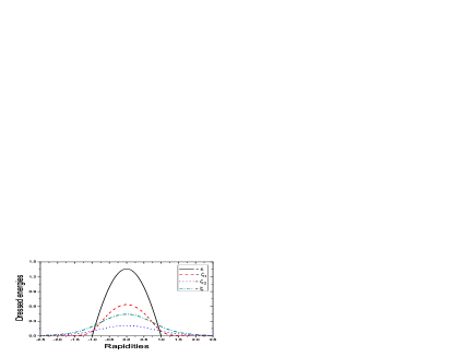
Figure 1: (Color online) The dressed energies of the ground state ($Q=1,\,c=1$). $\epsilon$, $\zeta_{1}$, $\zeta_{2}$ and $\xi$ are the dressed energies of rapidities $k$, real $\lambda$, 2-string $\lambda$ and real $\mu$, respectively. At the Fermi point $Q$, the dressed energy $\epsilon(Q)$ is zero.

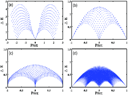
Figure 2: (Color online) The low-lying excitations ($c=1$, $Q=1$). $\Delta E$ and $P$ are the energy and the momentum carried by the excitation. (a) The charge-hole excitations. (b) The excitation of two holes of real $\lambda$. (c) The excitation of two holes of real $\mu$. (d) the excitation of four holes of $\lambda$ 2-string.

The low-lying excitations of the system can be studied systemically by adding particles, holes or strings into the ground state configuration of the rapidities. The excitation energy reads

$$\sl{\Delta E} = \sum_{j=1}^{n_{h}}\epsilon(k_{j}^{h})+\sum_{j=1}^{n_{p}}\epsilon(k_{j}^{p})+\sum_{j=1}^{m_{1}}\zeta_{1}(\lambda^{h}_{1,j})$$ (15)

$$+ \sum_{j=1}^{m_{2}}\zeta_{2}(\lambda^{h}_{2,j})+\sum_{j=1}^{m_{3}}\eta_{1}(\mu^{h}_{j}),$$

where $n_{h}$, $n_{p}$ and $m_{1,2,3}$ are the numbers of the charge holes, excited charges, holes in real $\lambda$ sea, in 2-string $\lambda$ sea and in real $\mu$ sea, respectively; $k_{j}^{h}$, $k_{j}^{p}$, $\lambda^{h}_{1,2,j}$ and $\mu^{h}_{j}$ are the positions of the corresponding charges and holes. Formally, the extra strings contribute nothing to the energy because the contribution of such strings is exactly canceled by the rearrangement of the Fermi sea. Some of the low-lying excitations are shown in Fig.2. The real $k$ charge-hole excitation in our case is similar to that of $SU(4)$-invariant Sutherland model as shown in Fig.2(a). However, the excitations in the spin sector are quite different from those of the Sutherland model. The spin quanta carried by the spin excitations reads

$$S=\frac{3}{2}m_{2}+2m_{3}+\sum_{l\geq 3}(2-l)m_{\lambda^{(l)}}+\sum_{t\geq 2}(1-t)m_{\mu^{(t)}},$$ (16)

where $m_{\lambda^{(l)}}$ and $m_{\mu^{(t)}}$ are the numbers of $\lambda$ $l$-strings and the $\mu$ $t$-strings formed in the excitations, respectively. We note the numbers of holes and strings added are not independent but satisfy some constraints determined by the BAE:

$$\Delta M_{1}^{1}=-m_{1}+\frac{1}{2}m_{2},$$

$$\Delta M_{1}^{2}=\frac{1}{2}m_{1}-\frac{3}{4}m_{2}-\frac{1}{2}m_{3}-\sum_{l\geq 3}m_{\lambda^{(l)}},$$ (17)

$$\Delta M_{2}^{1}=-\frac{1}{2}m_{2}-m_{3}-\sum_{t\geq 2}m_{\mu^{(t)}},$$

where $\Delta M_{1,2}^{l}$ (integers) indicate the number changes of $\lambda,\mu$ $l$-strings. Several possible hole configurations are listed in Table 1.

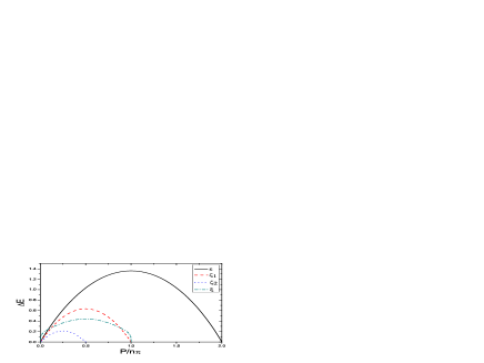
Figure 3: (Color online) The single-hole excitations ($Q=1$, $c=1$). $\Delta E$ and $P$ are the energy and the momentum carried by a single hole, respectively, and $n$ is the density of particles. The solid line is the single-hole excitation of real $k$. The dashed line is that of real $\lambda$. The dotted line is that of $\lambda$ 2-string and the dotted dashed line is that of real $\mu$.

Table 1: Possible hole configurations.

$m_{1}$	2	1	0	0	0	1
$m_{2}$	0	2	2	4	0	0
$m_{3}$	0	0	1	0	2	1

Nevertheless, the energies of the holes are additive as shown in Eq.(15) and the thermodynamic behavior of the system is mainly determined by the dispersion relations of the individual holes, which are shown in Fig.3. Interestingly, the single $\lambda$ 2-string hole carries the lowest energy with spin $3/2$ (named as heavy spinon) and therefore dominate the low temperature thermodynamics of the system.

The simplest spin excitation is a real $\lambda$ hole-pair (the first column in Table 1), corresponding to the two domain walls of a single excited domain. However, unlike the usual spinons, such holes carry zero spin (named as neutral spinons). The $\lambda$ 2-string hole pair can not exist independently but must be associated with a neutral spinon (the second column in Table 1) or a real $\mu$ hole (the third column in Table 1). If we add further a $\lambda$ 4-string into a 2-string hole pair and a real $\lambda$ hole configuration, the total spin of this excitation is 1. In this case each of the $\lambda$ 2-string holes carries a spin $1/2$. Such a dressed hole is quite similar to the ordinary spinon (named as dressed spinon). Four $\lambda$ 2-string holes may exist independently (the fourth column in Table 1). If we put further one $\lambda$ 6-string and one $\mu$ 3-strings into this four hole configuration, we get the $SO(5)$ spin singlet excitation. The simplest excitation in the $\mu$ sector is a pair of real $\mu$ holes (the fifth column in Table 1). This excitation is quite similar to a real $\lambda$ hole pair but each of the real $\mu$ hole carries a spin $2$. Joint pair of a real $\lambda$ hole and a real $\mu$ hole may also happen as shown in the last column in Table 1. Other kinds of spin excitations can be obtained by analyzing the BAE but most of the complex excitations are generally composed of the excitations listed in Table 1.

References

(1)
M. Greiner, et al., Phys. Rev. Lett. 87, 160405 (2001).
(2)
A. Gölitz, et al., Phys. Rev. Lett. 87, 130402 (2001).
(3)
F. Schreck, et al., Phys. Rev. Lett. 87, 080403 (2001).
(4)
H. Moritz, et al., Phys. Rev. Lett. 91, 250402 (2003).
(5)
T. Stöferle, et al., Phys. Rev. Lett. 92, 130403 (2004).
(6)
B.L. Tolra et al., Phys. Rev. Lett. 92, 190401 (2004).
(7)
T. Kinoshita, et al., Science 305, 1125 (2004).
(8)
B. Paredes, et al., Nature (London) 429, 277 (2004).
(9)
H. Moritz, et al., Phys. Rev. Lett. 94, 210401 (2005).
(10)
S. Aubin, et al., J. Low Temp. Phys. 140, 377 (2005).
(11)
T.L. Ho, Phys. Rev. Lett. 81, 742 (1998).
(12)
T. Ohmi and K. Machida, J. Phys. Soc. Jpn. 67, 1822 (1998).
(13)
M. Greiner, et al., Nature (London) 415, 39 (2002).
(14)
C.J. Myatt, et al., Phys. Rev. Lett. 78, 586 (1997).
(15)
D.M. Stamper-Kurn, et al., Phys. Rev. Lett. 80, 2027 (1998).
(16)
J. Cao, et al., Europhys. Lett. 79, 30005 (2007).
(17)
T.L. Ho and S. Yip, Phys. Rev. Lett. 82, 247 (1999).
(18)
C. Wu, et al., Phys. Rev. Lett. 91, 186402 (2003).
(19)
C. Wu, Phys. Rev. Lett. 95, 266404 (2005).
(20)
H.H. Tu, et al., Phys. Rev. B 74, 174404 (2006).
(21)
H.H. Tu, et al., Phys. Rev. B 76, 014438 (2007).
(22) P. Lecheminant, et al., Phys. Rev. Lett. 95, 240402 (2005).
(23)
D. Controzzi1 and A.M. Tsvelik, Phys. Rev. Lett. 96, 097205 (2006).
(24)
B. Sutherland, Phys. Rev. Lett. 20, 98 (1968).
(25)
P. Schlottmann, Int. J. Mod. Phys. B 11, 355 (1997).
(26)
W. Galleas and M.J. Martins, Nucl. Phys. B 768, 219 (2007).