Generation of GHZ and W states for stationary qubits in spin network via resonance scattering

Abstract

We propose a simple scheme to establish entanglement among stationary qubits based on the mechanism of resonance scattering between them and a single-spin-flip wave packet in designed spin network. It is found that through the natural dynamical evolution of an incident single-spin-flip wave packet in a spin network and the subsequent measurement of the output single-spin-flip wave packet, multipartite entangled states among $n$ stationary qubits, Greenberger-Horne-Zeilinger (GHZ) and W states can be generated with success probabilities $P_{GHZ}=2/|1+t^{-n}|^{2}$ and $P_{W}=\left|t\right|^{2}/n$ respectively, where $t$ is the transmission amplitude of the near-resonance scattering.

I Introduction

In quantum information science it is a crucial problem to develop techniques for generating entanglement among stationary qubits. Entanglement as unique feature of quantum mechanics can be used not only to test fundamental quantum-mechanical principles Bell ; Greenberger , but to play a central role in applications Ekert ; Deutsch ; Bennett . Especially, multipartite entanglement has been recognized as a powerful resource in quantum information processing and communication. There are two typical multipartite entangled states, Greenberger-Horne-Zeilinger (GHZ) and W states, which are usually referred to as maximal entanglement. Numerous protocols for the preparation of such states have been proposed Cirac ; Gerry ; Hagley ; Cabrillo ; Bose ; Lange ; Rauschenbeutel ; Zheng ; Feng ; Simon ; Zou ; Duan ; SongJ ; Su ; SongHS .

Most of them are scattering-based schemes which utilize two processes: the natural dynamic process of an always on system and the final project process carried out by a subsequent measurement. Another feature of such kind of schemes is that there are two kinds of qubits involved in: target qubits and flying qubit. The target qubits are the main entities that will be entangled by the above two processes, which are usually stationary and can be realized by atoms, impurities, or other quantum devices. The flying qubit is a mediator to establish the entanglement among the target qubits via the interaction between them, which is usually realized by photon or mobile electron.

In this sense, the type of interaction between stationary qubits and the flying qubit as a mediator and the transfer of the flying qubit are crucial for the efficiency of the entanglement creation. In general, such two processes are mutually exclusive. The scattering between stationary and flying qubits can convert information between them, while it also reduces the fidelity of the flying qubit, which will affect the efficiency of the entanglement, especially for multi-particle system. It is still a challenge to create entanglement among massive, or stationary qubits.

In this paper, we consider whether it is possible to use an arrangement of qubits, a spin network, to generate multipartite entanglement among stationary qubits via scattering process. We introduce a scheme that allow the generation of the GHZ and W states of stationary qubits in spin networks. In the proposed scheme, the flying qubit is a Gaussian type single-flip moving wave packet on the ferromagnetic background, which can propagate freely in $XY$ chain. The stationary qubit is consisted of two spins coupled by Ising type interaction with strength $J^{z}$. A single spin flip can be confined inside such two spins by local magnetic field $h$ to form a double-dot (DD) qubit. The system of an $XY$ spin chain with a DD qubit embedded in exhibits a novel feature under the resonance scattering condition $h=J^{z}$, that a single-flip moving wave packet can completely pass over a DD qubit and switch it from state $\left|0\right\rangle$ to $\left|1\right\rangle$ simultaneously. We show that the scattering between a flying qubit and a DD qubit can induce the entanglement between them and the operation on the DD qubit can be performed by the measurement of the output flying qubit. It allows simple schemes for generation of multipartite entanglement, such as GHZ and W states by simply-designed spin networks. We also investigate the influence of near-resonance effects on the success probabilities of the schemes. It is found that the success probabilities are $P_{GHZ}=$ $2\left|1+t^{-n}\right|^{2}$ and $P_{W}=\left|t\right|^{2}/n$ for the generation of GHZ and W states, respectively. Here $t$ is the transmission probability amplitude for a single DD qubit and $n$ is the number of the DD qubits.

This paper is organized as follows. In Sec. II the DD qubit and spin network are presented. In Sec. III we investigate the resonance-scattering process between the flying and stationary qubits. Sec. IV and V are devoted to the application of the resonance scattering on schemes of creating GHZ and W states. Section VI is the summary and discussion.

II Double-dot qubit

The spin network we consider in this paper is consisted of spins connected via the $XXZ$ interaction. The Hamiltonian is

$$H = -\sum_{\left\langle i,j\right\rangle}\left[\frac{J_{ij}^{\bot}}{2}(\sigma_{i}^{+}\sigma_{j}^{-}+\mathrm{H.c.})+J_{ij}^{z}\sigma_{i}^{z}\sigma_{j}^{z}\right]$$

$$+\sum_{i}h_{i}\sigma_{i}^{z},$$

where $\sigma_{i}^{\pm}=\sigma_{i}^{x}\pm i\sigma_{i}^{y}$, and $\sigma_{i}^{\alpha}$ $(\alpha=x,y,z)$ are the Pauli spin matrices for the spin at site $i$. The total $z$-component of spin, or the number of spin flips on the ferromagnetic background, is conserved as it commutes with the Hamiltonian. For $J_{ij}^{z}=0$, it reduces to $XY$ spin network, which has received a wide study for the purpose of quantum state transfer and creating entanglement between distant qubits by using the natural dynamics Bose Rev . For $J_{ij}^{z}=J_{ij}^{\bot}$, the Hamiltonian describes isotropic Heisenberg model. In the antiferromagnetic regime ($J_{ij}^{z}\prec 0$), a ladder geometry spin network, a gapped system LiY PRA , has been employed as a data bus for the swapping operation and generation of entanglement between two distant stationary qubits. It has been shown that a moving wave packet can act as a flying qubit Osborne ; Shi PRA ; Yang PRA like photon in a fiber. On the other hand, the analogues of optical device, beam splitter can be fabricated in quantum networks of bosonic Plenio , spin and ferimonic systems Yang EPJB .

In this paper, we consider a new type of qubit, double-dot qubit, which can be embedded in such spin networks. A DD qubit consists of two ordinary spins at sites $d$ and $d+1,$ connected via Ising type interaction in the form

$$H_{d}=-J^{z}\sigma_{d}^{z}\sigma_{d+1}^{z}+h\sum_{i=d,d+1}\sigma_{i}^{z}.$$ (2)

When such kinds of two spins are embedded in the spin networks with $\left|h\right|\gg J_{ij}^{\bot}$ and $h_{i}=0$, a spin flip is confined within it and forms a DD qubit with the notations $\left|0\right\rangle_{d}=\left|\downarrow\right\rangle_{d}\left|\uparrow\right\rangle_{d+1}$ and $\left|1\right\rangle=\left|\uparrow\right\rangle_{d}\left|\downarrow\right\rangle_{d+1}$. We will show that such a new type of qubit has a novel feature when it interacts with another spin flip in the spin networks.

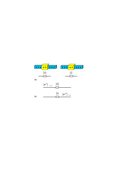
Figure 1: (Color online) The basic building block of the proposed scheme. (a) Schematic illustration for a DD qubit embedded in a spin chain, which consists of two spins with only Ising interaction. The local external magnetic field can confine a spin flip in the two spins to form a DD qubit with states $\left|0\right\rangle$ and $\left|1\right\rangle$. (b) Schematic illustration of the resonance scattering process between a single-spin-flip wave packet and a DD qubit. Under the resonance scattering condition, an incident wave packet can totally pass through a DD qubit and switch it from state $\left|0\right\rangle$ to state $\left|1\right\rangle.$ 

III Resonant scattering

The main building block in the spin network of our scheme is the DD qubit. It acts as a massive or stationary qubit, like atoms or ions in cavity-QED-based schemes. To demonstrate the property of a DD qubit in a spin chain, we investigate a small system of $4$-site, a DD qubit connecting to two spins. In order to provide a clear exposition, we firstly assume a specific coupling configuration with $h=J^{z}$, which leads to the following $4$-site Hamiltonian

$$H_{s} = -J^{\bot}\sum_{l=1,3}\left(\sigma_{l}^{x}\sigma_{l+1}^{x}+\sigma_{l}^{y}\sigma_{l+1}^{y}\right)$$

$$-h\sigma_{2}^{z}\sigma_{3}^{z}+h\left(\sigma_{2}^{z}+\sigma_{3}^{z}\right).$$

There is a quasi-invariant subspace with the diagonal energy being $h$ and under the condition $h\gg\left|J^{\bot}\right|$, which is spanned by basis

$$\left|\varphi_{1}\right\rangle = \left|\uparrow\right\rangle_{1}\left|\downarrow\right\rangle_{2}\left|\uparrow\right\rangle_{3}\left|\downarrow\right\rangle_{4},$$

$$\left|\varphi_{2}\right\rangle = \left|\downarrow\right\rangle_{1}\left|\uparrow\right\rangle_{2}\left|\uparrow\right\rangle_{3}\left|\downarrow\right\rangle_{4},$$ (4)

$$\left|\varphi_{3}\right\rangle = \left|\downarrow\right\rangle_{1}\left|\uparrow\right\rangle_{2}\left|\downarrow\right\rangle_{3}\left|\uparrow\right\rangle_{4}.$$

The matrix of the Hamiltonian in this subspace reads

$$\left[\begin{array}[]{ccc}h&-\frac{J^{\bot}}{2}&\\ -\frac{J^{\bot}}{2}&h&-\frac{J^{\bot}}{2}\\ &-\frac{J^{\bot}}{2}&h\end{array}\right]$$ (5)

with eigenstates $\left|\psi_{i}\right\rangle$ and eigen energies $\varepsilon_{i}$ $(i=1,2,3)$ being

$$\left|\psi_{1}\right\rangle = \frac{1}{\sqrt{2}}\left(\left|\varphi_{1}\right\rangle-\left|\varphi_{3}\right\rangle\right),\varepsilon_{1}=h;$$ (6)

$$\left|\psi_{2,3}\right\rangle = \frac{1}{2}\left(\left|\varphi_{1}\right\rangle\mp\sqrt{2}\left|\varphi_{2}\right\rangle+\left|\varphi_{3}\right\rangle\right),$$

$$\varepsilon_{2,3} = \pm\frac{1}{\sqrt{2}}J^{\bot}+h.$$

Obviously, in the invariant subspace, such a $4$-site system acts as a normal $3$-site system. Note that the DD qubit as the center of the $3$-site system can be in two different states $\left|0\right\rangle$ or $\left|1\right\rangle$ while another spin flip is at left or right site. Thus a time evolution process can accomplish the transformation $\left|\uparrow\right\rangle_{1}\left|\downarrow\right\rangle_{2}\left|\uparrow\right\rangle_{3}\left|\downarrow\right\rangle_{4}\longrightarrow\left|\downarrow\right\rangle_{1}\left|\uparrow\right\rangle_{2}\left|\downarrow\right\rangle_{3}\left|\uparrow\right\rangle_{4}$ or $\left|\uparrow\right\rangle_{1}\left|0\right\rangle_{d}\left|\downarrow\right\rangle_{4}\longrightarrow\left|\downarrow\right\rangle_{1}\left|1\right\rangle_{d}\left|\uparrow\right\rangle_{4}$ with 100% success probability. Such a feature is desirable for the quantum information processing. It is because that, on one hand, a spin flip passing over a DD qubit can operate the qubit state; and on the other hand, the state of a DD qubit can indicate whether there is a spin flip passing over it. A similar transformation has been proposed through the cavity input-output process in adiabatic limit Lee . A particular merit of the present scheme is that it is based on a natural dynamic process rather than an adiabatic process.

Now we consider the dynamic process of the interaction between a moving wave packet and a DD qubit. We embed a DD qubit into a chain as illustrated in Fig. 1(a). It has been shown that a single-spin-flip wave packet in the form Osborne ; Yang PRA

$$\left|\phi(\frac{\pi}{2},N_{c})\right\rangle=\frac{1}{\sqrt{\Omega}}\sum_{j}e^{-\frac{\alpha^{2}}{2}(j-N_{c})^{2}+i\frac{\pi}{2}j}\sigma_{j}^{+}\left|Vac\right\rangle$$ (7)

can propagate along a uniform spin chain without spreading approximately, where the vacuum state is fully ferromagnetic state $\left|Vac\right\rangle=\prod\nolimits_{l=1}\left|\downarrow\right\rangle_{l}$. Here $\Omega=\sum_{1}^{N}\exp(-\alpha^{2}(j-N_{c})^{2}/2)$ is the normalization factor, $N_{c}$ is the center of the wave packet at $t=0$ and $N$ is the number of sites of the chain. At time $t$, it will evolves to $\left|\phi(\pi/2,N_{c}+J^{\bot}t)\right\rangle$. Let us firstly assume that initially the qubit is in the state $\left|0\right\rangle_{d}$, while a wave packet of type (7) $\left|\phi(\pi/2,N_{c}\prec d)\right\rangle\equiv$ $\left|\phi(\pi/2,L)\right\rangle$ is coming from the left. Similarly, we define $\left|\phi(\pm\pi/2,N_{c}\succ d+2)\right\rangle$ $\equiv\left|\phi(\pm\pi/2,R)\right\rangle$, $\left|\phi(-\pi/2,N_{c}\prec d)\right\rangle$ $\equiv\left|\phi(-\pi/2,L)\right\rangle$ to denote a transmitted or reflected wave packet after scattering. In the strong local field regime, $h\gg\left|J^{\bot}\right|$, the spin flip is firmly confined in the DD qubit. From the analysis of the above $4$-site system, which is called the resonant case with $h=J^{z}$, the wave packet will pass freely through the DD qubit. Comparing to the case without the embedded DD qubit, the output wave packet gets a forward shift with a lattice space, while switches the DD qubit from $\left|0\right\rangle_{d}$ to $\left|1\right\rangle_{d}$, i.e.,

$$\left|\phi(\frac{\pi}{2},L)\right\rangle\left|0\right\rangle_{d}\longrightarrow\left|\phi(\frac{\pi}{2},R)\right\rangle\left|1\right\rangle_{d}.$$ (8)

In contrast, if the qubit is in state $\left|1\right\rangle$, the scattering process is

$$\left|\phi(\frac{\pi}{2},L)\right\rangle\left|1\right\rangle_{d}\longrightarrow\left|\phi(-\frac{\pi}{2},L)\right\rangle\left|1\right\rangle_{d},$$ (9)

i.e., the incoming wave packet is totally reflected and maintains the qubit to be in state $\left|1\right\rangle_{d}$. Interestingly, the states of wave packet and the DD qubit are both altered through this process, i.e., being shifted with a lattice space. However, such a shift brings about totally different effects on the DD qubit and the wave packet, respectively: it switches the DD qubit from $\left|0\right\rangle_{d}$ to $\left|1\right\rangle_{d}$, but does not alter the wave packet in the same manner as classical perfect elastic collision. It is worthy to point out that the DD qubit and the wave packet are not entangled in such resonant case. In the case of non-resonance $h\neq J^{z}$, or initially the DD qubit and/or the incident wave packet are in a superposition states as

$$\left|\nearrow\right\rangle_{d} = \alpha\left|0\right\rangle_{d}+\beta\left|1\right\rangle_{d},$$ (10)

$$\left|\nearrow\right\rangle_{in} = \alpha\left|\phi(\frac{\pi}{2},L)\right\rangle+\beta\left|Vac\right\rangle,$$

where $\alpha$ and $\beta$ are arbitrary coefficients satisfying $\left|\alpha\right|^{2}+\left|\beta\right|^{2}=1$.

In practice, the difference between $h$ and $J^{z}$ will leads to the reflection of the incident wave packet. Then the scattering process can be expressed as

$$\left|\phi(\frac{\pi}{2},L)\right\rangle\left|0\right\rangle_{d}\longrightarrow r\left|\phi(-\frac{\pi}{2},L)\right\rangle\left|0\right\rangle_{d}+t\left|\phi(\frac{\pi}{2},R)\right\rangle\left|1\right\rangle_{d}$$ (11)

with $\left|r\right|^{2}+\left|t\right|^{2}=1$. The transmission coefficient $T(J^{z},h)=\left|t\right|^{2}$ is a crucial factor in the following schemes for quantum information processing. On the other hand, the strength of the local field $h$ also results the spreading of the spin flip from state $\left|1\right\rangle_{d}$ and reduces $T(J^{z},h)$. We perform numerical simulation for the scattering process in order to investigate such phenomenon. Numerical result for $T(J^{z},h)$ with $\alpha=4/15$ is plotted in Fig. 2. It shows that the transmission coefficient is close to $1$ if $h\sim J^{z}\succ 5\left|J^{\bot}\right|$, which is feasible in practice. It ensures that a spin network with an embedded DD qubit in a spin chain can perform the transformation (8, 9) via a natural dynamic process rather than an adiabatic process.

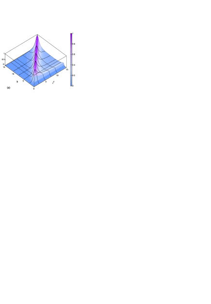
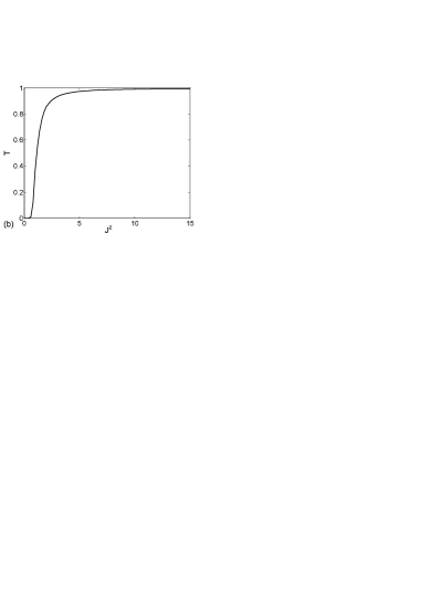
Figure 2: (Color online) Profiles of transmission coefficient $T$ as a function of $h$ and $J^{z}$ in the unit of $J^{\bot}$, obtained by numerical simulations. (a) 3-D plot of the function $T(h,J^{z})$. It indicates that the transmission coefficient gets the maxima under the resonance scattering condition $h=J^{z}$. (b) The plot of the transmission coefficient under the resonance scattering condition. It shows that the transmission coefficient is close to $1$ in the region $h\sim J^{z}\succ\left|5J^{\bot}\right|$.

IV Generation of GHZ state

Now we focus on the practical application of resonant scattering effect on the quantum information processing. As mentioned above, although the totally transmitted wave packet switches the state of the DD qubit from $\left|0\right\rangle_{d}$ to $\left|1\right\rangle_{d}$, there is no entanglement between the DD and the wave packet arising from such a process. However, if the incoming wave packet is not polarized in $z$ direction, but in the form

$$\left|\nearrow\right\rangle_{in}=\alpha\left|\phi(\frac{\pi}{2},L)\right\rangle+\beta\left|Vac\right\rangle,$$ (12)

where $\alpha$ and $\beta$ are restricted to be real for simplicity in the following context, the entanglement between the DD qubit and the scattered wave packet can be established. Actually, the corresponding resonant scattering process can be expressed as

$$\left|\nearrow\right\rangle_{in}\left|0\right\rangle_{d}\longrightarrow\alpha\left|1\right\rangle_{d}\left|\phi(\frac{\pi}{2},R)\right\rangle+\beta\left|0\right\rangle_{d}\left|Vac\right\rangle.$$ (13)

The reduced density matrix of the final state in the basis $\{\left|1\right\rangle_{d}\left|Vac\right\rangle$, $\left|1\right\rangle_{d}\left|\phi(\pi/2,R)\right\rangle$, $\left|0\right\rangle_{d}\left|Vac\right\rangle$, $\left|0\right\rangle_{d}\left|\phi(\pi/2,R)\right\rangle\}$ is

$$\left[\begin{array}[]{cccc}0&&&\\ &\alpha^{2}&\alpha\beta&\\ &\alpha\beta&\beta^{2}&\\ &&&0\end{array}\right],$$ (14)

which has concurrence $C=2\left|\alpha\beta\right|$. For $\alpha=\beta=1/\sqrt{2}$, the concurrence between them reaches to the maximum $C_{\max}=1$. A flying qubit (12) can be generated from wave packet (7) via a $1\times 2$-beam or $Y$-beam splitter Yang EPJB . We consider the spin network with the geometry of two connected $1\times 2$-beam splitters. These two $Y$-beam splitters are characterized by $\left(\alpha\text{, }\beta\right)$ and $\left(\alpha^{\prime}\text{, }\beta^{\prime}\right)$ respectively, which are schematically shown in Fig. 3(a). There is a DD qubit embedded in one of the two arms. Now we consider the dynamic process with the initial state being $\left|\psi^{in}\right\rangle\left|0\right\rangle_{d}$, where $\left|\psi^{in}\right\rangle=\left|\phi(\pi/2,-\infty)\right\rangle$, denotes an incoming wave packet along the left chain. In the first step, through the beam splitter $\left(\alpha\text{, }\beta\right)$, $\left|\psi^{in}\right\rangle$ is divided into two wave packets $\left|\phi(\pi/2,L)\right\rangle_{A}$ and $\left|\phi(\pi/2)\right\rangle_{B}$ along $A$ and $B$ arms, respectively. In the second step, sub-wave packet $\left|\phi(\pi/2,L)\right\rangle_{A}$ passes over DD qubit and becomes $\left|\phi(\pi/2,R)\right\rangle_{A}$, while sub-wave packet $\left|\phi(\pi/2)\right\rangle_{B}$ propagates along $B$ arm and meets $\left|\phi(\pi/2,R)\right\rangle_{A}$ at the joint of beam splitter $\left(\alpha^{\prime}\text{, }\beta^{\prime}\right)$. In the third step, wave packets $\left|\phi(\pi/2,R)\right\rangle_{A}$ and $\left|\phi(\pi/2)\right\rangle_{B}$ are reflected and divided by beam splitter $\left(\alpha^{\prime}\text{, }\beta^{\prime}\right)$, and contribute to the output wave packet $\left|\psi^{out}\right\rangle=\left|\phi(\pi/2,\infty)\right\rangle$. Then the whole process can be expressed as

$$\left|\psi^{in}\right\rangle\left|0\right\rangle_{d}$$ (15)

$$\overset{\text{step 1}}{\longrightarrow}\alpha\left|\phi(\frac{\pi}{2},L)\right\rangle_{A}\left|0\right\rangle_{d}+\beta\left|\phi(\frac{\pi}{2})\right\rangle_{B}\left|0\right\rangle_{d}$$

$$\overset{\text{step 2}}{\longrightarrow}\alpha\left|1\right\rangle_{d}\left|\phi(\frac{\pi}{2},R)\right\rangle_{A}+\beta\left|0\right\rangle_{d}\left|\phi(\frac{\pi}{2})\right\rangle_{B}$$

$$\overset{\text{step 3}}{\longrightarrow}\left(\alpha^{\prime}\alpha\left|1\right\rangle_{d}+\beta^{\prime}\beta\left|0\right\rangle_{d}\right)\left|\psi^{out}\right\rangle$$

$$+\left(\beta^{\prime 2}\alpha\left|1\right\rangle_{d}-\alpha^{\prime}\beta^{\prime}\beta\left|0\right\rangle_{d}\right)\left|\phi(-\frac{\pi}{2},R)\right\rangle_{A}$$

$$+\left(\alpha^{\prime 2}\beta\left|0\right\rangle_{d}-\alpha^{\prime}\beta^{\prime}\alpha\left|1\right\rangle_{d}\right)\left|\phi(-\frac{\pi}{2})\right\rangle_{B}.$$

From step 2 to step 3 we have used formulas (28, 29) derived in Appendix A. When $\left|\psi^{out}\right\rangle$ is measured in the output lead, the operation

$$\left|0\right\rangle_{d}\longrightarrow\alpha^{\prime}\alpha\left|1\right\rangle_{d}+\beta^{\prime}\beta\left|0\right\rangle_{d}$$ (16)

is implemented. The success probability of this operation is $\left(\alpha\alpha^{\prime}\right)^{2}+\left(\beta\beta^{\prime}\right)^{2}$. In the optimal case with $\alpha=\beta=\alpha^{\prime}$ $=\beta^{\prime}=1/\sqrt{2}$, we can perform the operation $\left|0\right\rangle_{d}\longrightarrow\left(\left|1\right\rangle_{d}+\left|0\right\rangle_{d}\right)/\sqrt{2}$ by the process of resonant scattering and subsequent measurement with the success probability up to $0.5$. The measurement of $\left|\psi^{out}\right\rangle$ can be implemented by embedding another DD qubit to record the passing of the output wave packet.

Now we consider the case of multiple DD qubits embedded in $A$ arm, which is schematically illustrated in Fig. 3(b). All the $n$ stationary DD qubits are prepared initially in state $\left|0\right\rangle^{\otimes n}=\prod\nolimits_{l=1}^{n}\left|0\right\rangle_{l}$. Similarly, we have

$$\left|\psi^{in}\right\rangle\left|0\right\rangle^{\otimes n}$$ (17)

$$\overset{\text{step 1}}{\longrightarrow}\alpha\left|\phi(\pi/2,L)\right\rangle_{A}\left|0\right\rangle^{\otimes n}+\beta\left|\phi(\frac{\pi}{2})\right\rangle_{B}\left|0\right\rangle^{\otimes n}$$

$$\overset{\text{step 2}}{\longrightarrow}\alpha\left|\phi(\pi/2,R)\right\rangle_{A}\left|1\right\rangle^{\otimes n}+\beta\left|\phi(\frac{\pi}{2})\right\rangle_{B}\left|0\right\rangle^{\otimes n}$$

$$\overset{\text{step 3}}{\longrightarrow}\left(\alpha^{\prime}\alpha\left|1\right\rangle^{\otimes n}+\beta^{\prime}\beta\left|0\right\rangle^{\otimes n}\right)\left|\psi^{out}\right\rangle$$

$$+\left(\beta^{\prime 2}\alpha\left|1\right\rangle^{\otimes n}-\alpha^{\prime}\beta^{\prime}\beta\left|0\right\rangle^{\otimes n}\right)\left|\phi(-\frac{\pi}{2},R)\right\rangle_{A}$$

$$+\left(\alpha^{\prime 2}\beta\left|0\right\rangle^{\otimes n}-\alpha^{\prime}\beta^{\prime}\alpha\left|1\right\rangle^{\otimes n}\right)\left|\phi(-\frac{\pi}{2})\right\rangle_{B},$$

with the notation $\left|1\right\rangle^{\otimes n}=\prod\nolimits_{l=1}^{n}\left|1\right\rangle_{l}$.

In the optimal case with $\alpha=\beta=\alpha^{\prime}$ $=\beta^{\prime}=1/\sqrt{2}$, we can perform the operation

$$\left|0\right\rangle^{\otimes n}\longrightarrow\frac{1}{\sqrt{2}}\left(\left|1\right\rangle^{\otimes n}+\left|0\right\rangle^{\otimes n}\right)$$ (18)

by the subsequent measurement with the success probability up to $0.5$. Then by using natural dynamics and subsequent measurement, multipartite entangled GHZ state can be generated. This provides a simple way of entangling $n$ stationary qubits through scattering with a flying qubit. In the near-resonance scattering case, the transmission probability amplitude $t$ will effect the success probability to be

$$P_{GHZ}=\frac{2}{\left|1+t^{-n}\right|^{2}},$$ (19)

under the optimal conditions $\alpha=\alpha^{\prime}=\sqrt{1/\left(1+t^{n}\right)}$, $\beta=\beta^{\prime}=\sqrt{t^{n}/\left(1+t^{n}\right)}$. Note that the success probability is reduced exponentially as the number of qubits increases.

V Generation of W state

Now we turn to the scheme of the generation of another type of multipartite entangled state, W state. The configuration of the spin network we utilized consists of two $1\times n$-beam splitters with one DD qubit embedded in each parallel arm in the same way, as illustrated in Fig. 3(c).

We start our analysis by considering $n=2$ case with two $1\times 2$-beam splitters being characterized by $\left(\alpha\text{, }\beta\right)$ and $\left(\alpha^{\prime}\text{, }\beta^{\prime}\right)$ respectively. Denoting the qubit states of two DD qubits embedded in arms $A$ and $B$ as $\left|0,1\right\rangle_{A}$ and $\left|0,1\right\rangle_{B}$ respectively, the dynamic process can be written as

$$\left|\psi^{in}\right\rangle\left|0\right\rangle_{A}\left|0\right\rangle_{B}$$ (20)

$$\overset{\text{step 1}}{\longrightarrow}\alpha\left|\phi(\frac{\pi}{2},L)\right\rangle_{A}\left|0\right\rangle_{A}\left|0\right\rangle_{B}+\beta\left|\phi(\frac{\pi}{2},L)\right\rangle_{B}\left|0\right\rangle_{A}\left|0\right\rangle_{B}$$

$$\overset{\text{step 2}}{\longrightarrow}\alpha\left|1\right\rangle_{A}\left|\phi(\frac{\pi}{2},R)\right\rangle_{A}\left|0\right\rangle_{B}+\beta\left|1\right\rangle_{B}\left|\phi(\frac{\pi}{2},R)\right\rangle_{B}\left|0\right\rangle_{A}$$

$$\overset{\text{step 3}}{\longrightarrow}\left(\alpha\alpha^{\prime}\left|1\right\rangle_{A}\left|0\right\rangle_{B}+\beta\beta^{\prime}\left|1\right\rangle_{B}\left|0\right\rangle_{A}\right)\left|\psi^{out}\right\rangle$$

$$+\left(\alpha\beta^{\prime 2}\left|1\right\rangle_{A}\left|0\right\rangle_{B}-\beta\alpha^{\prime}\beta^{\prime}\left|1\right\rangle_{B}\left|0\right\rangle_{A}\right)\left|\phi(-\frac{\pi}{2},R)\right\rangle_{A}$$

$$+\left(\beta\alpha^{\prime 2}\left|1\right\rangle_{B}\left|0\right\rangle_{A}-\alpha\alpha^{\prime}\beta^{\prime}\left|1\right\rangle_{A}\left|0\right\rangle_{B}\right)\left|\phi(-\frac{\pi}{2},R)\right\rangle_{B}.$$

In the optimal case with $\alpha=\beta=\alpha^{\prime}=\beta^{\prime}=1/\sqrt{2}$, we can perform the operation

$$\left|0\right\rangle_{A}\left|0\right\rangle_{B}\longrightarrow\frac{1}{\sqrt{2}}\left(\left|1\right\rangle_{A}\left|0\right\rangle_{B}+\left|0\right\rangle_{A}\left|1\right\rangle_{B}\right)$$ (21)

by the subsequent measurement of the output spin flip with the success probability up to $0.5$.

Now we extend the above conclusion to $n$-DD qubits case. For a $1\times n$-beam splitter, we only consider the simplest case with identical hopping constant being $J^{\bot}/2\sqrt{n}$ between the input lead and each arm, which is schematically illustrated in Fig. 3(c). An incident wave packet will experience the following process. In the first step, $\left|\psi^{in}\right\rangle$ is divided into $n$ wave packets through the beam splitter, with $\left|\phi(\pi/2,L)\right\rangle_{l}$ $\left(l=1,2,...,n\right)$ being the wave packet along the $l$th arm. In the second step, every sub-wave packet $\left|\phi(\pi/2,L)\right\rangle_{l}$ passes over the corresponding DD qubit embedded in the $l$th arm, and switches its state from $\left|0\right\rangle_{l}$ to $\left|1\right\rangle_{l}$ simultaneously. In the third step, all the sub-wave packets $\left|\phi(\pi/2,R)\right\rangle_{l}$ are reflected and divided at the node of the right beam splitter, and contribute to the output wave packet $\left|\psi^{out}\right\rangle=\left|\phi(\pi/2,\infty)\right\rangle$. The whole process can be expressed as

$$\left|\psi^{in}\right\rangle\left|0\right\rangle^{\otimes n}$$ (22)

$$\overset{\text{step 1}}{\longrightarrow}\frac{1}{\sqrt{n}}\sum_{l=1}^{n}\left|\phi(\frac{\pi}{2},L)\right\rangle_{l}\prod\nolimits_{l=1}^{n}\left|0\right\rangle_{l}$$

$$\overset{\text{step 2}}{\longrightarrow}\frac{1}{\sqrt{n}}\sum_{l=1}^{n}\left|\phi(\frac{\pi}{2},R)\right\rangle_{l}\left|1\right\rangle_{l}\prod\nolimits_{i\neq l}^{n}\left|0\right\rangle_{i}$$

$$\overset{\text{step 3}}{\longrightarrow}\frac{1}{n}\sum_{l=1}^{n}\left|1\right\rangle_{l}\prod\nolimits_{i\neq l}^{n}\left|0\right\rangle_{i}\left|\psi^{out}\right\rangle$$

$$-\frac{1}{n\sqrt{n}}\sum_{l=1}^{n}\sum_{j=1}^{n}\left|\psi_{j}^{out}\right\rangle\left|1\right\rangle_{l}\prod\nolimits_{i\neq l}^{n}\left|0\right\rangle_{i}$$

$$+\sum_{l=1}^{n}\left|\psi_{l}^{out}\right\rangle\left|1\right\rangle_{l}\prod\nolimits_{i\neq l}^{n}\left|0\right\rangle_{i}$$

From step 2 to step 3 we have used the formula (VII.2) derived in Appendix B. When $\left|\psi^{out}\right\rangle$ is measured in the output lead, the operation

$$\left|0\right\rangle^{\otimes n}\longrightarrow\frac{1}{\sqrt{n}}\sum_{l=1}^{n}\left|1\right\rangle_{l}\prod\nolimits_{i\neq l}^{n}\left|0\right\rangle_{i}$$ (23)

is implemented with the success probability $1/n$. Then by using natural dynamics and subsequent measurement, multipartite entangled W state can be generated. In the near-resonance scattering case, the transmission probability amplitude $t$ reduces the success probability to

$$P_{W}=\frac{\left|t\right|^{2}}{n}.$$ (24)

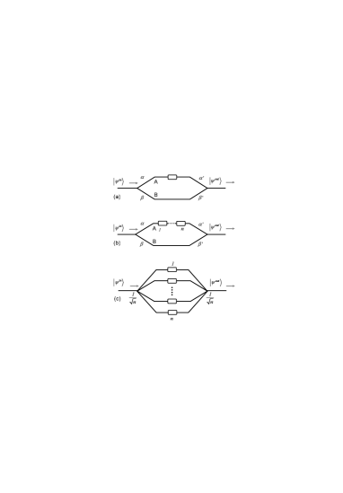
Figure 3: Schematic illustrations for the scheme of entanglement generation in spin network. (a) Realization of operation $\left|0\right\rangle\longrightarrow$ $(\left|1\right\rangle+\left|0\right\rangle/\sqrt{2}$. (b) Generation of the GHZ state. (c) Generation of the W state.

As the comparison of the success probabilities of creating GHZ and W states of $n$ qubits with the transmission coefficient $T$, we plot Eqs. (19) and (24) in Fig. 4 for the cases with $T=1.0$, $0.9$, $0.8$, and $0.7$; $n=2$, $3$, $...$, $8$. It shows that when $T$ is close to $1$, the difference between $P_{GHZ}$ and $P_{W}$ becomes large as $n$ increases. As $T$ decreases from $1$, the difference between $P_{GHZ}$ and $P_{W}$ becomes smaller for fixed $n$.

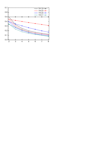
Figure 4: (Color online) Success probabilities for the generation of GHZ and W states of $n$ qubits in the system with transimission coefficient $T$.

VI Summary

We have shown how a spin network can be used to generate multipartite entanglement among stationary qubits. The key of this scheme is the alternative of massive or stationary qubit in a spin network, DD qubit. The resonance scattering between a DD qubit and a SFWP, which acts as the alternative of a flying qubit in a spin network, allows a perfect transformation: an incident wave packet can totally pass through a DD qubit and switch it from state $\left|0\right\rangle$ to state $\left|1\right\rangle$. The resonance scattering condition is investigated analytically and numerically. It shows that the resonance scattering is feasible in practice. This ensures that through the natural dynamical evolution of an incident single-spin-flip wave packet in a spin network and the subsequent measurement of the output single-spin-flip wave packet, multipartite entangled states among $n$ stationary qubits, GHZ and W states can be generated. There are two merits in our scheme. Firstly, the massive or stationary qubit, DD qubit, is constructed by the element, two neighbor spins of the spin network, which is applicable to all types of the scalable multi-qubit systems. Secondly, it is based on a natural dynamic process rather than an adiabatic process. There is certainly significant potential for spin networks to find applications in solid state quantum processing and communication.

We acknowledge the support of the CNSF (grant No. 10874091, 2006CB921205).

VII Appendix Dynamics of wave packets in beam splitters

In this appendix, we present the exact results for the dynamics of wave packets in beam splitters.

VII.1 Appendix A: $1\times 2$ beam splitter

In the work of Ref. Yang EPJB the dynamics of a wave packet in the spin networks based on the $XY$ model was studied. A $1\times 2$-beam splitter is consisted of three uniform spin chains with coupling constant $J^{\bot}/2$. The connections between three uniform chains are $\alpha J^{\bot}/2$ and $\beta J^{\bot}/2$ as in Fig. 5. It has been shown that under the condition $\alpha^{2}+\beta^{2}=1$, an input moving wave packet $\left|\psi^{in}\right\rangle$ will be divided into two wave packets $\left|\psi_{\alpha}^{out}\right\rangle$ and $\left|\psi_{\beta}^{out}\right\rangle$ without any reflection, which can be expressed as

$$\left|\psi^{in}\right\rangle\longrightarrow\alpha\left|\psi_{\alpha}^{out}\right\rangle+\beta\left|\psi_{\beta}^{out}\right\rangle.$$ (25)

Similarly, the inverse process also holds, i.e.,

$$\alpha\left|\psi_{\alpha}^{in}\right\rangle+\beta\left|\psi_{\beta}^{in}\right\rangle\longrightarrow\left|\psi^{out}\right\rangle,$$ (26)

where states $\left|\psi^{in}\right\rangle$, $\left|\psi_{\alpha}^{in}\right\rangle$, and $\left|\psi_{\beta}^{in}\right\rangle$ ($\left|\psi^{out}\right\rangle$, $\left|\psi_{\alpha}^{out}\right\rangle$, and $\left|\psi_{\beta}^{out}\right\rangle$) represent the wave packets coming in (out) of the node along the three chains respectively. Contrarily, for two wave packets along the two arms, which interference destructively at the node, we have

$$\beta\left|\psi_{\alpha}^{in}\right\rangle-\alpha\left|\psi_{\beta}^{in}\right\rangle\longrightarrow\beta\left|\psi_{\alpha}^{out}\right\rangle-\alpha\left|\psi_{\beta}^{out}\right\rangle.$$ (27)

Combining the above Eqs. (26 and 27), we have

$$\left|\psi_{\alpha}^{in}\right\rangle\longrightarrow\alpha\left|\psi^{out}\right\rangle+\beta^{2}\left|\psi_{\alpha}^{out}\right\rangle-\alpha\beta\left|\psi_{\beta}^{out}\right\rangle,$$ (28)

and

$$\left|\psi_{\beta}^{in}\right\rangle\longrightarrow\beta\left|\psi^{out}\right\rangle-\alpha\beta\left|\psi_{\alpha}^{out}\right\rangle+\alpha^{2}\left|\psi_{\beta}^{out}\right\rangle.$$ (29)

Then for a given incident wave packet along any branch of a $1\times 2$ beam splitter, the probability amplitudes of all the output wave packets can be obtained exactly.

VII.2 Appendix B: $1\times n$ beam splitter

Now we consider a $1\times n$ beam splitter consists of one chain of length $l_{a}$ and $n$ arms of length $l_{b}$ with identical connecting coupling strength $J^{\bot}/2\sqrt{n}$ for each arm, which is shown in Fig. 6. The Hamiltonian of such quantum network reads

$$\mathcal{H} = -\frac{J^{\bot}}{2}\sum_{i=1}^{l_{a}-1}a_{i}^{{\dagger}}a_{i+1}-\frac{J^{\bot}}{2\sqrt{n}}\sum_{l=1}^{n}a_{l_{a}}^{{\dagger}}b_{l,1}$$

$$-\frac{J^{\bot}}{2}\sum_{l=1}^{n}\sum_{j=1}^{l_{b}-1}b_{l,j}^{{\dagger}}b_{l,j+1}+\mathrm{H.c.},$$

where $a_{i}^{{\dagger}}$ and $b_{l,j}^{{\dagger}}$ are particle operators at site $i$ of chain $l_{a}$ and site $j$ of the arm $l$. They can be boson or fermion operators. The conclusion for such model is available for the dynamics of a single flip in the analogue of spin network.

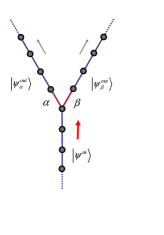
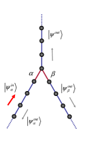
Figure 5: (Color online) Schematic illustration for a $1\times 2$ beam splitter. Left panel: an incident wave packet $|\psi^{in}\rangle$ is split into two sub-wave packets $|\psi_{\alpha}^{out}\rangle$ and $|\psi_{\beta}^{out}\rangle$ without any reflection. Right panel: an incident wave packet $|\psi_{\alpha}^{in}\rangle$, along one of the two arms is divided into three sub-wave packets $|\psi_{\alpha}^{out}\rangle$, $|\psi_{\beta}^{out}\rangle$ and $|\psi^{out}\rangle$.

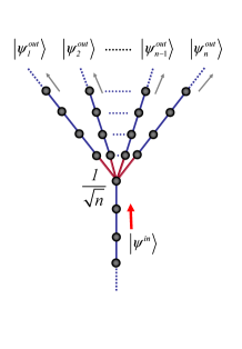
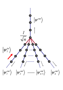
Figure 6: (Color online) Schematic illustration for a $1\times n$ beam splitter. Left panel: an incident wave packet $|\psi^{in}\rangle$, is split into $n$ sub-wave packets $|\psi_{j}^{out}\rangle$ $(j=1,...,n)$ without any reflection. Right panel: an incident wave packet $|\psi_{l}^{in}\rangle$ along one of the $n$ arms is divided into $n+1$ sub-wave packets $|\psi_{j}^{out}\rangle$ $(j=1,...,n)$ and $|\psi^{out}\rangle$. 

Similarly as shown in Ref. Yang EPJB , we can perform the following transformations

$$c_{i}^{{\dagger}} = a_{i}^{{\dagger}},\left(i\leq l_{a}\right),$$ (31)

$$c_{i+l_{a}}^{{\dagger}} = \frac{1}{\sqrt{n}}\sum_{j=1}^{n}b_{j,i}^{{\dagger}},\left(i\leq l_{b}\right),$$

$$d_{l,i}^{{\dagger}} = \frac{1}{\sqrt{n}}\sum_{j=1}^{n}e^{-i\frac{2\pi l}{n}j}b_{j,i}^{{\dagger}},\left(l=1,2,...,n-1\right),$$

where $c_{i}^{{\dagger}}$ and $d_{l,j}^{{\dagger}}$ are also corresponding boson or fermion operators. Under the transformations, Hamiltonian (VII.2) can be written as

$$\mathcal{H} = \mathcal{H}_{c}+\sum_{l=1}^{n-1}\mathcal{H}_{l},$$ (32)

$$\mathcal{H}_{c} = -\frac{J^{\bot}}{2}\sum_{i=1}^{l_{a}+l_{b}-1}\left(c_{i}^{{\dagger}}c_{i+1}+\mathrm{H.c.}\right),$$

$$\mathcal{H}_{l} = -\frac{J^{\bot}}{2}\sum_{i=1}^{l_{b}-1}\left(d_{l,i}^{{\dagger}}d_{l,i+1}+\mathrm{H.c.}\right),$$

$$\left(l=1,2,..,n-1\right).$$

Note that the sub-Hamiltonians satisfy

$$\left[\mathcal{H}_{c},\mathcal{H}_{l}\right]=0,\left[\mathcal{H}_{l},\mathcal{H}_{m}\right]=0,$$ (33)

which indicate that the original quantum network, $1\times n$ beam splitter can be decomposed into $n$ independent chains, one of them is the length of $l_{a}+l_{b}$ and the rest are all the length of $l_{b}$. Based on the fact that a moving wave packet can propagate freely along the $n$ independent chains, we have the following processes

$$\left|\psi^{in}\right\rangle \longrightarrow \frac{1}{\sqrt{n}}\sum_{j=1}^{n}\left|\psi_{j}^{out}\right\rangle,$$ (34)

$$\frac{1}{\sqrt{n}}\sum_{j=1}^{n}\left|\psi_{j}^{in}\right\rangle \longrightarrow \left|\psi^{out}\right\rangle,$$

$$\sum_{j=1}^{n}e^{-i\frac{2\pi m}{n}j}\left|\psi_{j}^{in}\right\rangle \longrightarrow \sum_{j=1}^{n}e^{-i\frac{2\pi m}{n}j}\left|\psi_{j}^{out}\right\rangle,$$

$$\left(m=1,2,..,n-1\right).$$

Through a straightforward algebra, we obtain a set of expressions

$$\left|\psi_{l}^{in}\right\rangle \longrightarrow \frac{1}{\sqrt{n}}\left|\psi^{out}\right\rangle-\frac{1}{n}\sum_{j=1}^{n}\left|\psi_{j}^{out}\right\rangle+\left|\psi_{l}^{out}\right\rangle,$$

$$\left(l=1,2,..,n\right).$$

Then for a given incident wave packet along any branch of a $1\times n$ beam splitter, the probability amplitudes of all the output wave packets can be obtained exactly.

References

-
(1)
emails: songtc@nankai.edu.cn
- (2) J. S. Bell, Physics (Long Island City, N.Y.) 1, 195 (1965).
- (3) D. M. Greenberger, M.A. Horne, A. Shimony, and A. Zeilinger, Am. J. Phys. 58, 1131 (1990).
- (4) A. K. Ekert, Phys. Rev. Lett. 67, 661 (1991).
- (5) D. Deutsch and R. Jozsa, Proc. R. Soc. London A 439, 553 (1992).
- (6) C. H. Bennett, G. Brassard, C. Crepeau, R. Jozsa, A. Peres, and W. K. Wootters, Phys. Rev. Lett. 70, 1895 (1993).
- (7) J. I. Cirac and P. Zoller, Phys. Rev. A 50, R2799 (1994).
- (8) C. C. Gerry, Phys. Rev. A 53, 2857 (1996).
- (9) E. Hagley, X. Maitre, G. Nogues, C. Wunderlich, M. Brune, J. M. Raimond, and S. Haroche, Phys. Rev. Lett. 79, 1 (1997).
- (10) C. Cabrillo, J. I. Cirac, P. Garcia-Fernandez, and P. Zoller, Phys. Rev. A 59, 1025 (1999).
- (11) S. Bose, P. L. Knight, M. B. Plenio, and V. Vedral, Phys. Rev. Lett. 83, 5158 (1999).
- (12) W. Lange and H. J. Kimble, Phys. Rev. A 61, 063817 (2000).
- (13) A. Rauschenbeutel, G. Nogues, S. Osnaghi, P. Bertet, M. Brune, J. Raimond, and S. Haroche, Science 288, 2024 (2000).
- (14) S. B. Zheng, Phys. Rev. Lett. 87, 230404 (2001).
- (15) X. L. Feng, Z. M. Zhang, X. D. Li, S. Q. Li, S. Q. Gong, and Z. Z. Xu, Phys. Rev. Lett. 90, 217902 (2003).
- (16) C. Simon and W. T. M. Irvine, ibid. 91, 110405 (2003).
- (17) X. B. Zou, K. Pahlke, and W. Mathis, Phys. Rev. A 68, 024302 (2003).
- (18) L. M. Duan and H. J. Kimble, Phys. Rev. Lett. 90, 253601 (2003).
- (19) J. Song, Y. Xia, H. S. Song, J. L. Guo, and J. Nie, Europhys. Lett. 80, 60001 (2007).
- (20) X. Su, A. Tan, X. Jia, J. Zhang, C. Xie, and K. Peng, Phys. Rev. Lett. 98, 070502 (2007).
- (21) Y. Xia, J. Song, and H.S. Song, Appl. Phys. Lett. 92, 021127 (2008).
- (22) S. Bose; Contemporary Physics 48, 13 (2007), and references therein.
- (23) Y. Li, T. Shi, B. Chen, Z. Song, C.P. Sun, Phys. Rev. A 71, 022301 (2005); M.X. Huo, Ying Li, Z. Song and C.P. Sun, Europhys. Lett. 84 30004 (2008).
- (24) T. J. Osborne and N. Linden, Phys. Rev. A 69, 052315 (2004).
- (25) L. F. Wei, X. Li, X. Hu, and F. Nori, Phys. Rev. A 71, 022317 (2005).
- (26) T. Shi, Ying Li, Z. Song and C.P. Sun, Phys. Rev. A 71, 032309 (2005).
- (27) M. B. Plenio, J. Hartley, and J. Eisert, New J. Phys. 7, 73 (2004); A. Perales and M. B. Plenio, J. Opt. B 7, S601 (2005).
- (28) S. Yang, Z. Song and C. P. Sun, Eur. Phys. J. B 52, 377 (2006); S. Yang, Z. Song and C. P. Sun, Front. Phys. China 1, 1 (2007).
- (29) J. Lee, J. Park, S.M. Lee, H.W. Lee, and A.H. Khosa, Phys. Rev. A 77, 032327 (2008).