Limited-Rate Channel State Feedback for Multicarrier Block Fading Channels

Abstract

The capacity of a fading channel can be substantially increased by feeding back channel state information from the receiver to the transmitter. With limited-rate feedback what state information to feed back and how to encode it are important open questions. This paper studies power loading in a multicarrier system using no more than one bit of feedback per sub-channel. The sub-channels can be correlated and full channel state information is assumed at the receiver. First, a simple model with $N$ parallel two-state (good/bad) memoryless sub-channels is considered, where the channel state feedback is used to select a fixed number of sub-channels to activate. The optimal feedback scheme is the solution to a vector quantization problem, and the associated performance for large $N$ is characterized by a rate distortion function. As $N$ increases, we show that the loss in forward rate from the asymptotic (rate-distortion) value decreases as $(\log N)/N$ and $\sqrt{(\log N)/N}$  with optimal variable- and fixed-rate feedback codes, respectively. We subsequently extend these results to parallel Rayleigh block fading sub-channels, where the feedback designates a set of sub-channels, which are activated with equal power. Rate-distortion feedback codes are proposed for designating subsets of (good) sub-channels with Signal-to-Noise Ratios (SNRs) that exceed a threshold. The associated performance is compared with that of a simpler lossless source coding scheme, which designates groups of good sub-channels, where both the group size and threshold are optimized. The rate-distortion codes can provide a significant increase in forward rate at low SNRs.

I Introduction

Multicarrier transmission techniques, including orthogonal frequency-division multiplexing (OFDM), provide a convenient way to exploit frequency diversity in multipath fading channels. Given the total transmit power, a substantial increase in the channel capacity can be achieved if the power allocation across the sub-channels is adapted to channel variations [1]. For example, consider the sum capacity of $N$ independent block Rayleigh fading sub-channels with given total power or Signal-to-Noise Ratio (SNR). If the power is equally spread over all $N$ sub-channels, the capacity is upper bounded by the total SNR regardless of $N$, whereas if the power is allocated according to (optimal) water-filling, the capacity increases as $O(\log N)$ as $N$ increases [2, 3].

The state or quality of the sub-channels is typically measured at the receiver and sent to the transmitter through a feedback channel. We refer to this as channel state feedback (CSF). Obviously, optimal power allocation requires a prohibitive (infinite) amount of CSF in case of continuous channel state. Even if the channel state can be discretized, the number of sub-channels may exceed the total number of feedback bits. Hence, what state information to feed back and how to encode the feedback are important questions.

This work studies the use of limited CSF for maximizing the achievable rate of multicarrier block fading channels. It is assumed that the sub-channel states are known or can be measured accurately at the receiver. The channel state is encoded using fewer than one bit per sub-channel and then sent to the transmitter through a noiseless feedback channel. The transmitter chooses a subset of sub-channels to activate based on the feedback.

The problem of encoding the feedback is essentially a vector quantization (VQ) problem, where the channel state is mapped to a given number of bits for later reconstruction. Unlike the usual quantization problem, the reconstruction here is to produce a power loading vector for the sub-channels, where the distortion metric is the gap between the rate achieved using the feedback and the capacity achieved with known channel state at the transmitter.

Multicarrier power allocation with limited-rate feedback has been previously considered in [4, 5, 6, 2]. In particular, [4] applies the Lloyd algorithm to produce a codebook of power loading vectors, which maximizes an objective such as achievable rate. Unfortunately, the size of the codebook in [4], and hence the search complexity, grows exponentially with the amount of feedback. Other heuristic schemes with one bit feedback per sub-channel have been proposed in [2, 5, 3].

This paper investigates the trade-off between the forward data rate and the amount of CSF for block-fading multicarrier channels assuming no more than one bit of feedback per sub-channel. Furthermore, in contrast with the lossless feedback source coding schemes analyzed in [2], here we consider the more general class of lossy (rate-distortion) source codes.

We first consider a model with two fading states only. Each sub-channel randomly assumes either a good or bad state during a coherence block. For the case of independent two-state sub-channels studied in Section II, the role of the feedback is to direct the transmitter to select as many good sub-channels as possible to activate subject to the power constraint. The fundamental trade-off between the feedback rate and the sum capacity can be characterized using rate distortion theory in the limit of infinite number of sub-channels. For given finite number of sub-channels, we also quantify the gap between rates achievable by random coding and the rate distortion bound. Specifically, with variable-rate feedback codes the gap decreases as $(\log N)/N$, whereas with fixed-rate codes the gap decreases as $\sqrt{(\log N)/N}$.

We also compare the rate-distortion approach with a simple lossless source coding scheme, which reports as many good sub-channels as the feedback rate allows. Numerical plots show that good codes in the rate distortion sense typically achieve much higher forward rate. The result is then extended to the case of correlated two-state sub-channels in Section III, where the sub-channel states are assumed to form a Markov chain. Upper and lower bounds on the forward rate are derived as a function of the feedback rate.

With the insights gained from the two-state channel model, we then study the problem of limited CSF for Rayleigh fading sub-channels. The fading coefficient, or state of each sub-channel is a Circularly Symmetric Complex Gaussian (CSCG) random variable during each coherence block. The case of independent sub-channels is studied in Section IV whereas the case of correlated sub-channels is discussed in Section V. The state of each sub-channel is first reduced to a binary variable by comparing its gain with a threshold. Similar feedback codes as considered for the two-state channels is used to instruct the transmitter which sub-channels to activate, assuming the power is distributed evenly over the activated sub-channels. The threshold is selected to maximize the forward rate given a fixed feedback rate. It turns out that the trade-off admits a similar characterization as that for two-state sub-channels. Although reduction of Rayleigh states to binary states induces loss, the scheme with optimized threshold and a moderate amount of feedback performs close to optimal water-filling with channel coefficients known at the transmitter. In particular, given a total power constraint, the scheme can achieve a forward rate, which has the same order of increase with the number of sub-channels as that of water-filling [2].

Two heuristic lossless source schemes for the reduced (two-state) version of the Rayleigh channel are also considered for comparison in Section IV. In particular, in one of the schemes, taken from [7], the sub-channels are divided evenly into groups and the feedback indicates the set of groups in which all sub-channel gains exceed the threshold. A binary state vector, indicating which groups to activate, is then compressed using lossless source coding and fed back to the transmitter. The group size and threshold can be adjusted to maximize the forward achievable rate, subject to the feedback rate constraint. Such grouping, or clustering, of sub-channels to reduce feedback overhead has also been studied in [8] in a multiuser setting. Clustering sub-channels to reduce the training overhead and peak-to-average power ratio was previously studied in [9]. We characterize the growth in achievable rate with the number of sub-channels (for large $N$) as a function of the amount of feedback (which can also scale with $N$). Numerical examples show that the analytical results are quite accurate for finite-size systems of interest. In general, these heuristic schemes achieve a smaller forward rate than for the rate-distortion schemes, given a fixed feedback rate.

II Independent Two-state Sub-channels

Consider a bank of $N$ independent and statistically identical block fading sub-channels. During each coherence block, each sub-channel randomly takes one of two states, namely “good” and “bad,” which is known to the receiver. The input is constrained such that up to a fraction $p$ of the sub-channels can be activated by the transmitter. Suppose on average the amount of CSF is limited to $R_{f}$ bits per sub-channel per coherence block. The problem is to design a feedback scheme to maximize the forward data rate, i.e., to activate as many good sub-channels as possible.

II-A The Fundamental Trade-off via Rate Distortion Theory

Let the state of sub-channel $i$ be denoted by a Bernoulli random variable $S_{i}$, with the probability of being a good state denoted as ${\mathsf{P}}\left\{S_{i}=1\right\}=q$. Further, let the power loading variable $\hat{S}_{i}=1$ if the $i^{th}$ sub-channel is chosen to be activated and $\hat{S}_{i}=0$ otherwise. Constrained by the feedback and transmission power, a feedback scheme specifies a mapping from the set of binary channel state vectors, whose Hamming weight is no greater than $pN$.

It is easy to see that the feedback scheme is no different than vector quantization, where the channel state vector ${\boldsymbol{S}}=[S_{1},\dots,S_{N}]$ is mapped to $NR_{f}$ bits for recovery at the transmitter. Constrained by the feedback rate, the reconstruction may be prone to errors, and the quantization scheme should be designed to achieve as few errors (or, as small a distortion) in reconstruction as possible.

The fundamental trade-off of the forward and feedback rates as $N\rightarrow\infty$ can be addressed using rate distortion theory. The source is a sequence of independent and identically distributed (i.i.d.) Bernoulli$(q)$ random variables, $S_{1},S_{2},\dots$. The distortion measure can be described as $d_{N}({\boldsymbol{s}},\hat{{\boldsymbol{s}}})=\frac{1}{N}\sum^{N}_{i=1}d(s_{i},\hat{s}_{i})$ with

$$\textstyle d(s,\hat{s})=1_{\left\{{s>\hat{s}}\right\}}=\begin{cases}1,\quad\text{if }s=1\text{ and }\hat{s}=0,\\ 0,\quad\text{otherwise}.\end{cases}$$ (1)

The metric accounts for missed opportunities, i.e., good sub-channels which are not activated, but does not penalize activation of bad sub-channels, which we refer to as misfires. Further, the power loading vector has to satisfy a normalized weight constraint:

$$w(\hat{{\boldsymbol{s}}})=\frac{1}{N}\sum^{N}_{i=1}\hat{s}_{i}\leq p.$$ (2)

This additional challenge of incorporating the weight constraint on the reconstruction distinguishes the problem from the classical rate distortion problem concerning i.i.d. source and single-letter distortion measure. Though not obvious, the rate distortion problem admits the following simple single-letter characterization.

Theorem 1

For an i.i.d. Bernoulli($q$) source, given the weight constraint on every binary reconstruction, $w(\hat{{\boldsymbol{s}}})\leq p$, and the distortion measure, $d(s,\hat{s})=1_{\left\{{s>\hat{s}}\right\}}$, the rate distortion function is

$$R(D)=\min_{P_{\hat{S}|S}:\,\begin{subarray}{c}\mathsf{E}\,d(S,\hat{S})\leq D\\ {\mathsf{P}}\{\hat{S}=1\}\leq p\end{subarray}}I(S;\hat{S})$$ (3)

where $S\sim$ Bernoulli$(q)$.

Proof:

The achievability part of the theorem is based on Shannon’s random coding technique (see e.g., [10]). Fix $P_{\hat{S}|S}$ and some $0<\delta_{1}<p$, which satisfy $\mathsf{E}\,d(S,\hat{S})\leq D$ and ${\mathsf{P}}\{\hat{S}=1\}\leq p-\delta_{1}$. The code book of $2^{NR_{f}}$ codewords can be produced randomly with the marginal distribution $P_{\hat{S}}$. Further, an exponentially small fraction of codewords which violate the weight constraint (2) are purged. It can be shown that for sufficiently large code length $N$, the random codebook achieves the distortion $D$ as long as the rate $R>I(S_{i};\hat{S}_{i})+\delta_{2}$. The achievability part is thus proved because $\delta_{1}$ and $\delta_{2}$ can be chosen to be arbitrarily small.

Showing the converse requires incorporating the weight constraint (2) into the standard technique of [10]. Let $\hat{{\boldsymbol{S}}}$ represent the reconstruction of the random source vector ${\boldsymbol{S}}$. Consider any code of length $N$ with rate $R$ which satisfies the distortion and average weight constraints $\mathsf{E}[w(\hat{{\boldsymbol{S}}})]\leq p$, which is a weaker than required in the theorem. Then, due to the data processing theorem and the independence of $S_{i}$,

$$NR \geq I({\boldsymbol{S}};\hat{{\boldsymbol{S}}})$$ (4)

$$\geq\sum^{N}_{i=1}I(S_{i};\hat{S}_{i})$$ (5)

$$\geq\min_{P_{\hat{{\boldsymbol{S}}}|{\boldsymbol{S}}}:\,\begin{subarray}{c}{\mathsf{E}}\left\{\frac{1}{N}\sum^{N}_{i=1}\hat{S}_{i}\right\}\leq p\\ {\mathsf{E}}\left\{\frac{1}{N}\sum^{N}_{i=1}d(S_{i},\hat{S}_{i})\right\}\leq D\end{subarray}}\sum^{N}_{i=1}I(S_{i};\hat{S}_{i}).$$ (6)

The key task here is to break down the constraints on the distribution of the vector $\hat{{\boldsymbol{S}}}$ in (6) into constraints on the individual random variables. Note that $P_{\hat{{\boldsymbol{S}}}}$ is linear in $P_{\hat{{\boldsymbol{S}}}|{\boldsymbol{S}}}$ because the source distribution $P_{{\boldsymbol{S}}}$ is fixed. An important fact is that $I(S_{i};\hat{S}_{i})$ is convex in the distribution $P_{\hat{S}_{i}|S_{i}}$. Because of the symmetry in the indexes $i$, any optimal distribution $P_{\hat{{\boldsymbol{S}}}|{\boldsymbol{S}}}$ that achieves the minimum of (6) must be symmetric over all indexes $i$. Otherwise replacing all of them by their average yields smaller mutual information. Therefore, due to the symmetry and the additive nature of the constraints, (6) implies that the rate $R$ is lower bounded by $R(D)$ given in (3). ∎

The minimization over the conditional distribution $P_{\hat{S}|S}$ in (3) is equivalently over the crossover probabilities:

$$\epsilon_{0}=P_{\hat{S}|S}(0|1)\;\text{ and }\;\epsilon_{1}=P_{\hat{S}|S}(1|0),$$ (7)

where $\epsilon_{0}$ represents the probability of missing a good sub-channel. The mutual information $I(S;\hat{S})$ can be expressed as the following function of $(\epsilon_{0},\epsilon_{1})$:

$$i(\epsilon_{0},\epsilon_{1})\triangleq H_{2}(p)-qH_{2}(\epsilon_{0})-(1-q)H_{2}(\epsilon_{1}),$$ (8)

where $H_{2}(\cdot)$ stands for the binary entropy function. Unless stated otherwise, the units of all information metrics are bits. Note that the weight constraint (2) should be tight at the minimum because there is no penalty on misfires. Thus the optimal crossover probabilities satisfy $q(1-\epsilon_{0})+(1-q)\epsilon_{1}=p$.

Let the capacity of a good sub-channel be $C_{1}$ and the capacity of a bad sub-channel be $C_{0}<C_{1}$. The average number of active good sub-channels is $Nq(1-\epsilon_{0})$. The trade-off between the capacity and the feedback rate is characterized by as follows.

Proposition 1

Given $p$, $q$, and the feedback rate $R_{f}$ bits per sub-channel per coherence block, the maximum achievable forward data rate per sub-channel is

$$C=q(1-\epsilon_{0}^{*})(C_{1}-C_{0})+pC_{0},$$ (9)

where the optimal proportion of missed good sub-channels $\epsilon_{0}^{*}$ is the solution to the following optimization problem:

minimize: $$\quad\epsilon_{0}$$ (10a)

subject to: $$\quad H_{2}(p)-qH_{2}(\epsilon_{0})-(1-q)H_{2}(\epsilon_{1})\leq R_{f},$$ (10b)

$$\quad q(1-\epsilon_{0})+(1-q)\epsilon_{1}=p,$$ (10c)

$$\quad 0\leq\epsilon_{0},\epsilon_{1}\leq 1.$$ (10d)

The optimization problem (10) can be easily solved numerically. Clearly, the maximum forward data rate increases as the feedback rate increases, but the return vanishes beyond a certain point. The minimum feedback rate necessary for achieving the capacity can be determined by tentatively removing the feedback constraint (10b). If $p\geq q$, one can activate all good sub-channels so that $\epsilon_{0}=0$ with $\epsilon_{1}=\frac{p-q}{1-q}$, whereas if $p<q$, then $\epsilon_{0}$ can be as small as $1-\frac{p}{q}$ by choosing $\epsilon_{1}=0$. Substituting these values into (8), the forward rate saturates at the maximum feedback rate,

$$\overline{R}=\begin{cases}H_{2}(p)-qH_{2}\left(\frac{p}{q}\right),&\textrm{if }p\leq q,\\ H_{2}(1-p)-(1-q)H_{2}\left(\frac{1-p}{1-q}\right),&\textrm{if }p>q.\end{cases}$$ (11)

For any $R_{f}\leq\overline{R}$, the constraint (10b) is tight and $\epsilon_{0}^{*}$ can be calculated by solving the simultaneous equations (10b) and (10c), which can be easily reduced to a fixed-point equation.

II-B Performance Bounds for Finite Number of Sub-channels

Proposition 1 characterizes the asymptotic trade-off as the number of sub-channels $N$ goes to infinity. For a practical situation with finite $N$, the result needs refinement. Note that the solution to Proposition 1 provides an upper bound on the forward data rate for finite $N$, because the converse shown in the proof of Theorem 1 holds for all $N$. In the following, we consider random feedback codes and derive a lower bound for the achievable forward data rate with given feedback constraint.

II-B1 Fixed-Length Constant-Composition Feedback Code

Note that the solution to Proposition 1 upper bounds the forward data rate with the average input power constraint $E[w(\hat{{\boldsymbol{S}}})]=p$ and average feedback rate of $Ni(\epsilon_{0},\epsilon_{1})$ bits per coherence block. Here we impose two additional constraints without loss of generality: 1) The binary reconstruction vectors have constant composition, that is, $w(\hat{{\boldsymbol{s}}})=p$ for all the vectors $\hat{{\boldsymbol{s}}}$ in the feedback codebook; and 2) The feedback is at most $Ni(\epsilon_{0},\epsilon_{1})$ bits every coherence block. The second restriction implies that there are at most $2^{i(\epsilon_{0},\epsilon_{1})N}$ codewords.

The following proposition gives a lower bound on the achievable forward rate given these additional constraints.

Proposition 2

Let the number of feedback bits per coherence block be $N\,i(\epsilon_{0},\epsilon_{1})$, where $\epsilon_{0},\epsilon_{1}>0,\not=0.5$ are the solution to (10). Then $\exists\,N_{o}<\infty$ such that for $N\geq N_{o}$, the ergodic capacity achieved with the fixed-length constant-composition feedback code is lower bounded as

$$C_{fixed}\geq\left(1-2\sqrt{\frac{\log(Nq)}{Nq}}\right)C$$ (12)

where $C$ is given by (9).

The proof is given in Appendix A. The proposition implies that, for large enough $N$, the difference between the upper bound (9) and achievable forward rate per sub-channel approaches zero at the rate $O\big{(}\sqrt{(\log N)/N}\,\big{)}$. This further implies that the sum rate across the $N$ sub-channels incurs a loss, which increases as $O\big{(}\sqrt{N\log N}\,\big{)}$ compared to $NC$. The proof basically follows the random coding technique of Goblick [11] for analyzing the convergence rate of the rate distortion function for general sources and fixed-length block codes. The contribution in this work is to incorporate the additional constant-composition constraint and to simplify the analysis by exploiting the binary structure of the source and the reconstruction.

Although the result in Proposition 2 is stated for large $N$, more refined lower bound is derived in Appendix A which holds for any finite $N$.

II-B2 Variable-Length Feedback Codes

We note that fixed-length codes can cover a subset of most probable channel state vectors, but are unable to adapt to deviations from typical channel conditions. In the following, we analyze the performance of variable-length feedback codes. A variable amount of feedback is allowed during each coherence block as long as the average number of feedback bits is $Ni(\epsilon_{0},\epsilon_{1})$. The instantaneous power constraint is replaced by an average power constraint.

Proposition 3

Let the average number of feedback bits per coherence block be $Ni(\epsilon_{0},\epsilon_{1})$, where $\epsilon_{0},\epsilon_{1}>0$ are the solution to Proposition 1 and $\epsilon_{0},\epsilon_{1}\neq\frac{1}{2}$. Then $\exists\,N_{1}<\infty$ such that for every $N\geq N_{1}$, the ergodic forward rate achieved with a variable-length feedback code, under an average input power constraint $E[w(\hat{{\boldsymbol{S}}})]=p$, is lower bounded as

$$C_{var}\geq\left(1-\frac{6}{q[H_{2}^{\prime}(\epsilon_{0})+H_{2}^{\prime}(\epsilon_{1})]}\frac{\log_{2}N}{N}\right)C$$ (13)

where $C$ is given in (9).

The proof is provided in Appendix B. We follow the technique given by Pinkston [12], albeit with slight modifications. The main difference lies in incorporating the average input power constraint and avoiding the use of partition functions by exploiting the binary structure of the state and power loading vectors.

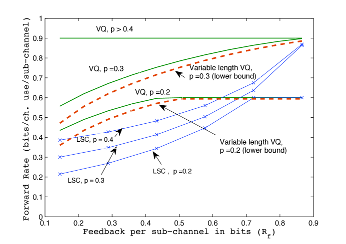
Figure 1: Forward rate versus feedback rate for different input constraints corresponding to VQ and sub-optimal feedback schemes using lossless source coding with channel state reduction (curves labeled with “LSC”). The sub-channels are assumed to be independent. Other parameters are $q=0.3$, $C_{1}=3$ and $C_{0}=0$. Also shown is the lower bound on forward rate corresponding to $N=500$ and a variable-length feedback code (dotted lines).

The proposition says that in this scenario the forward rate converges to the upper bound (9) as $O\left((\log N)/N\right)$. This is a substantial improvement over the $O\big{(}\sqrt{(\log N)/{N}}\big{)}$ convergence rate achieved by the fixed-length constant composition feedback codes (cf. (12)). Although the result in Proposition 3 is stated for large $N$, a more refined lower bound is derived in Appendix B, which holds for any finite $N$. Fig. 1 plots a few instances of this lower bound against the upper bound (9) as the feedback rate varies. Clearly, the lower bound is fairly close to the optimal forward rate (9) and becomes tighter as the feedback rate increases.

II-C Practical CSF Codes

Until now, we have shown that for moderate to large $N$, the rate distortion trade-off can be approached using random codes. Such a code, however, is not practical. As aforementioned, the Lloyd algorithm can be used to design a near-optimal vector quantizer for small number of sub-channels (see [13, 14, 4, 15] and references therein). Such a task becomes infeasible with tens or hundreds of sub-channels, as is the case in many applications.

One practical solution in the case of a large number of sub-channels is to use a graphical code similar to a low-density parity-check (LDPC) code. Encoding and decoding of the source (channel state vector) are respectively analogous to iterative decoding and encoding of a graphical error-control code. The complexity of such a code is in general linear in the number of sub-channels. For a discussion of graphical codes for source coding, the reader is referred to [16, 17, 18]. It is more challenging to design and implement variable-length codes.

II-D A Sub-optimal Scheme: Lossless Source Coding with Channel State Reduction

For comparison, we also consider a feedback scheme using simple channel state reduction and lossless source coding in lieu of vector quantization (henceforth referred to as the “LSC” scheme for convenience). If the feedback rate is greater than the entropy rate of the channel state vector, i.e., $R_{f}>H_{2}(q)$, then any lossless codes such as the Huffman code basically suffice. If the feedback rate is less than the entropy rate, we consider a simple scheme which reports a fraction $f$ of good sub-channels, where $f$ is chosen such that the entropy rate $H_{2}(fq)$ is basically $R_{f}$. On average the transmitter is informed of $fqN$ good sub-channels. The forward rate achieved with this option is

$$C_{f}=\begin{cases}p\,C_{1}\ ,&\textrm{if $p\leq fq$}\\ fqC_{1}+(p-fq)\,\frac{q(1-f)C_{1}+(1-q)C_{0}}{q(1-f)+(1-q)}\ ,&\textrm{otherwise}.\end{cases}$$ (14)

The expression follows directly from the observation that if fewer than fraction $p$ of the sub-channels are reported as good (that is, $fq<p$), the remaining $p-fq$ fraction of the sub-channels are chosen at random so that the probability of transmitting on a good sub-channel is given by $(q-fq)/(1-fq)$.

Note that it might be more efficient for the receiver to inform the transmitter to avoid a subset of bad sub-channels than to report a subset of good sub-channels, depending on the parameters. Suppose a fraction $\bar{f}$ of the bad sub-channels are reported to the transmitter where $H_{2}(\bar{f}(1-q))=R_{f}$. The forward rate achieved with this option is given by

$$\bar{C}_{f}=\begin{cases}p\frac{qC_{1}+(1-\bar{f})(1-q)C_{0}}{q+(1-\bar{f})(1-q)}\ ,&\textrm{if $p<q+(1-\bar{f})(1-q)$}\\ qC_{1}+(p-q)C_{0}\ ,&\textrm{otherwise}.\end{cases}$$ (15)

The maximum forward data rate achievable by the LSC scheme is therefore $\max\{C_{f},\bar{C}_{f}\}$.

II-E Numerical Results

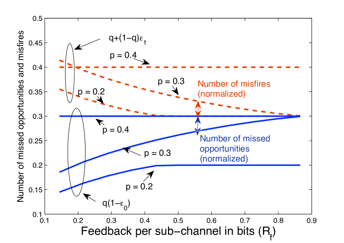
Figure 2: The number of misfires and missed opportunities (normalized by the total number of sub-channels $N$) versus the feedback rate for different input constraints. The sub-channels are assumed to be independent. Other parameters are $q=0.3$, $C_{1}=3$ and $C_{0}=0$.

We study the asymptotic performance of the optimal VQ scheme (given by (9)) and the sub-optimal LSC scheme (given by (14) and (15)). Fig. 1 plots the forward rate per sub-channel versus the feedback rate $R_{f}$ for different values of the input power constraint $p$. The LSC scheme is clearly inferior compared to the asymptotic VQ scheme with infinite as well as the variable-length VQ scheme at $N=500$ sub-channels. At small values of feedback, the VQ scheme gives substantial gains (up to $100\%$). The asymptotic result is quite representative of the performance with a relatively large number of sub-channels ($N=500$). As expected, the forward rate increases with the feedback amount and saturates at $R_{f}=H_{2}(q)$, at which point all good sub-channels can be reported at no loss.

The gain achieved with VQ can be better understood by studying the corresponding numbers of missed opportunities and misfires shown in Fig. 2. Intuitively, the larger the values of $\epsilon_{0}$ and $\epsilon_{1}$, the more “distortion” or “errors” we allow in the rate-distortion feedback code and hence it will require smaller amount of feedback. This is clearly reflected in (8). Consider the case of $p=0.4$ $(>q)$ in Fig. 2, $\epsilon_{0}=0$ and the fraction of misfires $(1-q)\epsilon_{1}=0.1$, which implies that we allow enough misfires so that the required feedback rate is kept small. In contrast, with $p=0.4$ we never report a bad sub-channel as good for the LSC scheme, and thereby incur extra feedback overhead. The reverse holds for $p=0.2$ $(<q)$, where the optimal scheme allows enough missed opportunities ($\epsilon_{0}$ is large and $\epsilon_{1}$ is small) so that the required feedback rate is again small. Since in this case $\epsilon_{1}\approx 0$, bad channels are not reported as good.

III Correlated Two-State Sub-channels

In multicarrier systems, the states of the sub-channels are often correlated. Consider the same system as in Section II except that the binary (good/bad) channel states of the $N$ sub-channels, $S_{1},S_{2},\dots,S_{N}$ form a stationary Markov chain. The optimal feedback scheme is nonetheless a vector quantization problem, with its asymptotic performance characterized by the following rate distortion result.

Theorem 2

Given a stationary binary Markov source $\{S_{i}\}$, a weight constraint on every binary reconstruction $w(\hat{{\boldsymbol{s}}})\leq p$, and the single-letter distortion measure $d(s,\hat{s})=1_{s>\hat{s}}$, the rate distortion function is given by

$$R(D)=\limsup_{N\to\infty}\min_{P_{\hat{{\boldsymbol{S}}}|{\boldsymbol{S}}}:\,\begin{subarray}{c}\sum{\mathsf{P}}\{\hat{S}_{i}=1\}\leq pN\\ \sum\mathsf{E}[d(S_{i},\hat{S}_{i})]\leq DN\end{subarray}}\frac{1}{N}\,I({\boldsymbol{S}};\hat{{\boldsymbol{S}}})$$ (16)

It is straightforward to prove Theorem 2 using the same techniques as developed in [19], with the additional weight constraint for the reconstruction. Hence the proof is omitted. Random codes achieve the rate distortion function. However, in practice, graphical codes can be designed to approach the optimal trade-off. In addition, Theorem 2 continues to hold if the instantaneous input constraint $w(\hat{{\boldsymbol{s}}})\leq p$ is replaced by an average input constraint $\mathsf{E}[w(\hat{{\boldsymbol{S}}})]\leq p$.

Note that (16) involves minimization over the conditional distribution of the entire power loading vector, and hence is not a single-letter characterization of the rate distortion function. Calculating the rate distortion function for correlated sources is a hard problem in general. The solution is known only in a few special cases pertaining to source alphabets, correlation models and distortion measures [19]. Even for a symmetric binary Markov chain and Hamming distortion, the rate distortion function is exactly known only for very small distortion values [20]. In the CSF problem, the reconstruction $\hat{{\boldsymbol{S}}}$ is a binary hidden Markov process. There is no known close-form expression for the entropy rate of such processes, although there exist approximations and numerical results in some cases (see, e.g., [21, 22] and references therein).

Since the exact solution to the optimization problem (16) is difficult, we will next find upper and lower bounds on the rate for a given distortion. Due to the stationarity of the source, the optimal conditional probability $P_{\hat{{\boldsymbol{S}}}|{\boldsymbol{S}}}$ is also stationary. Consider any stationary process $\{(S_{i},\hat{S}_{i})\,|\,i=0,\pm 1,\dots\}$ which satisfies the constraints in (16), i.e., ${\mathsf{P}}\{\hat{S}_{i}=1\}\leq p$ and $\mathsf{E}[d(S_{i},\hat{S}_{i})]\leq D$. Then

$$\lim_{N\rightarrow\infty}\frac{1}{N}I({\boldsymbol{S}};\hat{{\boldsymbol{S}}}) =\lim_{N\rightarrow\infty}\frac{1}{N}\sum^{N-1}_{i=1}I(S_{i};\hat{{\boldsymbol{S}}}|{\boldsymbol{S}}^{i-1}_{0})$$ (17)

$$=H(S_{1}|S_{0})-\lim_{N\rightarrow\infty}\frac{1}{N}\sum^{N-1}_{i=1}H(S_{i}|\hat{{\boldsymbol{S}}},{\boldsymbol{S}}^{i-1}_{0})$$ (18)

$$\geq H(S_{1}|S_{0})-H(S_{1}|\hat{S}_{1},S_{0})$$ (19)

$$=I(S_{1};\hat{S}_{1}|S_{0})$$ (20)

where (19) is because of stationarity and because conditioning decreases the entropy. The rate distortion function can thus be lower bounded as

$$R(D)\geq\min_{P_{\hat{S}_{1}|S_{1},S_{0}}}I(S_{1};\hat{S}_{1}|S_{0})$$ (21)

with $P_{\hat{S}_{1}|S_{1},S_{0}}$ satisfying the constraints in (16). The bounding mutual information depends only on the following four probabilities for the given source: $q_{s_{0}s_{1}}=P_{\hat{S}_{1},S_{0},S_{1}}(0,s_{0},s_{1})$ with $s_{0},s_{1}=0\text{ or }1$. Denote the lower bound by $i_{l}(q_{00},q_{01},q_{10},q_{11})=I(S_{1};\hat{S}_{1}|S_{0})$. This bound can be expressed as a function of the crossover probabilities denoted by $\delta_{01}={\mathsf{P}}\left\{S_{i}=1|S_{i\pm 1}=0\right\}$ and $\delta_{10}={\mathsf{P}}\left\{S_{i}=0|S_{i\pm 1}=1\right\}$ for all $i$. (The probability of a sub-channel being good is then $q=\delta_{01}/(\delta_{01}+\delta_{10})$) An explicit expression for the lower bound is derived in Appendix C.

In terms of these joint probabilities, the fraction of sub-channels that are good, and are correctly reported as good is given by $(q-q_{01}-q_{11})$ and the total fraction of sub-channels reported as good is given by $1-(q_{00}+q_{01}+q_{10}+q_{11})$. Consequently, an upper bound on the forward achievable rate can be obtained as the solution to the following optimization problem:

maximize: $$\quad(C_{1}-C_{0})(q-q_{01}-q_{11})+pC_{0}$$ (22a)

subject to: $$\quad 1-(q_{00}+q_{01}+q_{10}+q_{11})\leq p$$ (22b)

$$\quad i_{l}(q_{00},q_{01},q_{10},q_{11})\leq R_{f}$$ (22c)

$$\quad 0\leq q_{00},q_{01},q_{10},q_{11}\leq 1$$ (22d)

which can be easily solved numerically.

In order to find an upper bound on the rate distortion function, we restrict the minimization over $P_{\hat{{\boldsymbol{S}}}|{\boldsymbol{S}}}$ in (16) to be a minimization over a finite-dimensional distribution. For example, suppose that conditioned on $S_{i}$ and $S_{i+1}$, the random variable $\hat{S}_{i}$ is independent of all the remaining random variables in $({\boldsymbol{S}},\hat{{\boldsymbol{S}}})$. By stationarity and the Markovian property, the joint distribution of $({\boldsymbol{S}},\hat{{\boldsymbol{S}}})$ is determined by the conditional distribution $P_{\hat{S}_{0}|S_{0},S_{1}}$. Then it can be shown that, conditioned on $S_{i-1},S_{i+1},\hat{S}_{i-1}$ and $\hat{S}_{i}$, the variable $S_{i}$ is also independent of all the remaining random variables in ${\boldsymbol{S}}$ and $\hat{{\boldsymbol{S}}}$. Consequently,

$$H(S_{i}|\hat{{\boldsymbol{S}}},{\boldsymbol{S}}_{0}^{i-1}) \geq H(S_{i}|\hat{{\boldsymbol{S}}},{\boldsymbol{S}}_{0}^{i-1},{\boldsymbol{S}}_{i+1}^{N})$$ (23)

$$=H(S_{i}|S_{i-1},S_{i+1},\hat{S}_{i-1},\hat{S}_{i}).$$ (24)

Substituting in (18), an upper bound for the rate distortion function is obtained as the solution to the following optimization problem:

$$R(D)\leq\min_{P_{\hat{S}_{0}|S_{0},S_{1}}}I(S_{1};S_{2},\hat{S}_{0},\hat{S}_{1}|S_{0})$$ (25)

where $P_{\hat{S}_{0}|S_{0},S_{1}}$ is also subject to the constraints in (16). A simpler but looser bound is obtained if we assume that $\hat{S}_{i}$ is independent of everything else conditioned on $S_{i}$, for which the mutual information in (25) becomes $I(S_{1};S_{2},\hat{S}_{1}|S_{0})$, and the minimization is over $P_{\hat{S}_{0}|S_{0}}$. Again, let the crossover probabilities be given by (7). The upper bound is a function of these two crossover probabilities and is denoted by $i_{u}(\epsilon_{0},\epsilon_{1})=I(S_{1};S_{2},\hat{S}_{1}|S_{0})$. An explicit expression is derived in Appendix C. Consequently, a lower bound on the forward achievable rate can be obtained by solving an optimization problem similar to that in Proposition 1 with the constraint (10b) replaced by $i_{u}(\epsilon_{0},\epsilon_{1})\leq R_{f}$.

It is easily seen that if no reconstruction errors are allowed, then both the upper and lower bounds reduce to the entropy rate of the channel state process. In other word, if $H(\hat{{\boldsymbol{S}}}|{\boldsymbol{S}})=0$, or equivalently, $\epsilon_{0}=\epsilon_{1}=0$, $q_{10}=q_{00}=1$ and $q_{01}=q_{11}=0$, then $i_{l}(1,0,1,0)=i_{u}(0,0)=H(S_{1}|S_{0})$. Next we provide an example in which the upper bound is not tight. Choosing $p=1$ implies that the power loading vector $\hat{{\boldsymbol{S}}}$ can be chosen all ones and that achieves the capacity with zero feedback rate. However, equivalently choosing $\epsilon_{0}=0$ and $\epsilon_{1}=1$ gives the upper bound on required feedback rate $i_{u}(0,1)>0$.

Fig. 3 plots the upper and lower bounds on achievable forward rate per sub-channel versus $R_{f}$ for different values of $q$ with $\delta_{10}=0.3$ and $p=0.3$. Consider the plot for $q=0.3$. There is a substantial gap between the two bounds for small feedback rates. However, as the feedback rate increases, the gap closes and the bounds provide an accurate measure of the performance of the VQ scheme with correlated sub-channels. Also shown is the performance of the VQ scheme with independent sub-channels. Clearly, correlation improves the forward rate by decreasing the feedback requirement.

Later in Section V, the preceding methodology will be utilized to derive bounds on the performance of VQ schemes for correlated Rayleigh fading sub-channels.

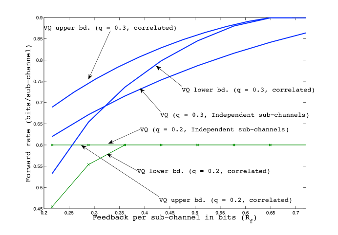
Figure 3: Upper and lower bounds on the forward rate with VQ versus the feedback rate for correlated sub-channels. Parameters are $\delta_{10}=0.3,p=0.3,C_{1}=3$ and $C_{0}=0$.

IV Independent Rayleigh fading sub-channels

The design of a limited-rate CSF strategy for Rayleigh fading sub-channels is again a VQ problem. Unfortunately, the exact distortion measure, which corresponds to the capacity-maximizing power loading vectors is difficult to work with [13, 14, 4, 15]. In order to simplify the problem, we focus on threshold-based schemes, which converts the sequence of Rayleigh fading sub-channels to a sequence of “good” (sub-channel gain above the threshold) and “bad” (sub-channel gain below the threshold) sub-channels. This enables the use of the limited feedback schemes developed for two-state sub-channels. It will be shown that, as the number of sub-channels $N\to\infty$, the rate achieved with such a scheme grows at the same rate as that of water-filling with full channel state information at the transmitter.

The limited feedback problem here differs from the case of two-state sub-channels studied in Sections II and III in two key aspects. First, the threshold which determines the fraction of sub-channels that are considered good needs to be optimized. Second, given the total power, the fraction of sub-channels to activate also influence the amount of powers in each active sub-channel.

IV-A System Model

Consider a multicarrier channel with $N$ independent and statistically identical, where the channel output for the $i$-th sub-channel is written as

$$Y_{i}=H_{i}X_{i}+Z_{i}$$ (26)

where $H_{i}$ and $Z_{i}$ are zero-mean circularly symmetric complex Gaussian (CSCG) random variables. Without loss of generality, we assume that the channel and noise variance is one, that is, $E[|H_{i}|^{2}]=E[|Z_{i}|^{2}]=1$. Also, the noise is assumed to be independent across the sub-channels. The $N\times 1$ input vector ${\boldsymbol{X}}=[X_{1},X_{2},\ldots,X_{N}]^{\dagger}$ satisfies the average total signal-to-noise ratio (SNR) constraint $E\left[{\boldsymbol{X}}^{\dagger}{\boldsymbol{X}}\right]\leq P$. The channel vector ${\boldsymbol{H}}=[H_{1},H_{2},\ldots,H_{N}]^{\dagger}$ is assumed to be known perfectly at the receiver. We assume a block fading model so that ${\boldsymbol{H}}$ remains constant for $T$ channel uses and then changes to an independent value. The time dependence is suppressed to simplify notation.

IV-B Optimal Threshold Based VQ

The gain for the $i$-th sub-channel, $|H_{i}|^{2}$, is exponentially distributed with its mean equal to one. Given a threshold $t\geq 0$, define the $N\times 1$ binary state vector ${\boldsymbol{S}}$ so that the $i$-th entry $S_{i}=1$ if $|H_{i}|^{2}\geq t$, and $S_{i}=0$ otherwise. The probability of a sub-channel being “good” is denoted as $q={\mathsf{P}}\left\{S_{i}=1\right\}={\mathsf{P}}\left\{|H_{i}|^{2}>t\right\}=e^{-t}$.

Suppose that, on average, the transmitter transmits over or, activates a fraction $p$ of the sub-channels. The power is distributed uniformly over the active sub-channels so that each transmission occurs with SNR equal to $P/(Np)$. Therefore, the expected capacity of a good and bad sub-channel, respectively, is given by

$$C_{1}=\frac{1}{q}\int_{t}^{\infty}e^{-\tau}\log\left(1+\frac{P\tau}{Np}\right)\text{d}\tau$$ (27)

and

$$C_{0}=\frac{1}{1-q}\int_{0}^{t}e^{-\tau}\log\left(1+\frac{P\tau}{Np}\right)\text{d}\tau.$$ (28)

Assume that on average $R_{f}$ bits per sub-channel per coherence block are available for error-free CSF. Also, define $B=NR_{f}$ as the average amount of feedback summed across all sub-channels. Similar to the case of two-state sub-channels, the power loading with limited CSF can be seen as a mapping from the space of channels state vector ${\boldsymbol{S}}$ to the space of power loading vectors $\hat{{\boldsymbol{S}}}$, where $\hat{S}_{i}=1$ if the $i$-th sub-channel is activated and $\hat{S}_{i}=0$ otherwise.

We note a key difference between the VQ problem at hand and the usual stationarity assumption in rate distortion theory: The optimal choice of the threshold $t$ here may vary with the total number of sub-channels, hence so does the statistics of the binary source denoted by probability $q$. Nonetheless, the following asymptotic bound on achievable distortion (equivalently, forward rates) can be established.

Proposition 4

Given $N$ parallel Rayleigh fading sub-channels and an average of $R_{f}$ bits of feedback per sub-channel per coherence block, the following statements hold.

1. The forward rate per sub-channel achieved with a threshold-based feedback scheme is upper bounded by $C$, the maximized objective in the following optimization problem:

   maximize: $$\quad C=q(1-\epsilon_{0})(C_{1}-C_{0})+pC_{0}$$ (29a)

   subject to: $$\quad H_{2}(p)-qH_{2}(\epsilon_{0})-(1-q)H_{2}(\epsilon_{1})\leq R_{f}$$ (29b)

   $$\quad q(1-\epsilon_{0})+(1-q)\epsilon_{1}=p$$ (29c)

   $$\quad 0\leq\epsilon_{0},\epsilon_{1}\leq 1$$ (29d)

   with $q=e^{-t}$, and where the maximization is over $p,t$ and $\epsilon_{0}$.

2. There exist fixed-length constant composition feedback codes which achieve the forward rate per sub-channel given by (12) with sufficiently large $N$, where $C$ and $q$ are obtained from solving the optimization problem in part (a).

3. There exist variable-length feedback codes which achieve the forward rate per sub-channel given by (13) with sufficiently large $N$, where $C$, $q$, $\epsilon_{0}$ and $\epsilon_{1}$ are obtained by solving the optimization problem in part (a).

Part (a) in Proposition 4 follows directly from the Fano’s inequality and is similar to that of Proposition 1. Note that the upper bound $C$ holds for any finite $N$. The lower bounds in parts (b) and (c) can be proved similarly as Propositions 2 and 3, respectively, corresponding to two-state sub-channels. The proofs are omitted. Although the lower bounds are stated for large $N$, more accurate expressions that apply to any finite $N$ are derived in Appendices A and B.

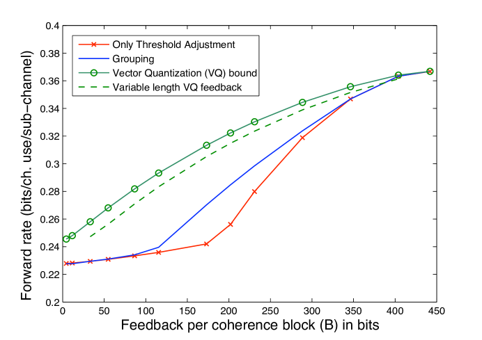
Figure 4: Forward rate versus feedback rate for different feedback schemes for $N=500$ sub-channels at SNR $P=20$ dB. For comparison, the water-filling capacity with full channel state information at receiver is 0.385 bits per sub-channel use.

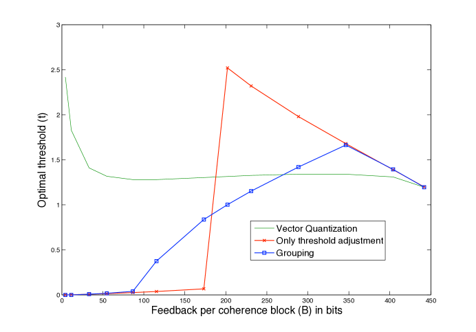
Figure 5: Optimal threshold versus feedback for different feedback schemes with SNR = 20 dB and N = 500.

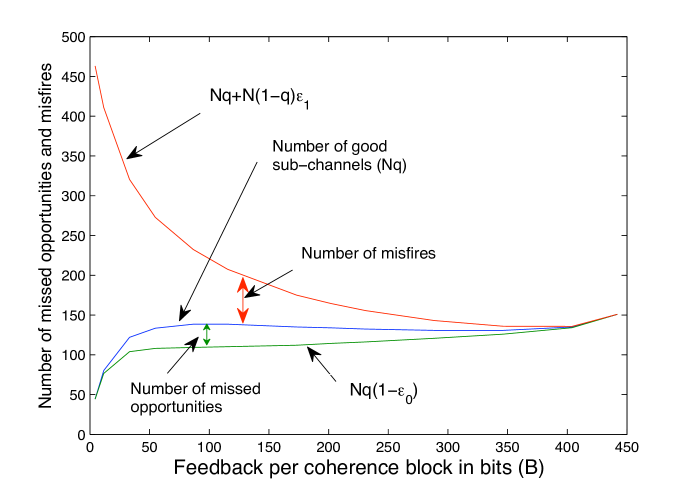
Figure 6: Optimal number of sub-channels that exceed the threshold together with the optimal number of missed opportunities and misfires corresponding to the VQ feedback scheme for independent Rayleigh fading sub-channels. Other parameters are SNR = 20 dB and N = 500.

Interestingly, (12) and (13) imply that the rate at which the lower bounds approach $C$ depends on the average number of good sub-channels $Nq$, which can be much smaller than the total number of sub-channels $N$. The upper and lower bounds on forward rate versus total feedback $B=NR_{f}$ per coherence block are shown in Fig. 4 for SNR $P=20$ dB.’ Only the lower bound corresponding to a variable-length variable composition feedback code is shown. Unless specified otherwise, here and in the subsequent numerical results we let $N=500$. The plots show that the upper and lower bounds are quite close (within 10%). The corresponding optimal threshold is shown in Fig. 5. The number of good sub-channels, number of missed opportunities and the number of misfires as a function of amount of feedback are shown in Fig. 6. Interestingly, for $B\geq 70$ bits, the threshold does not change significantly but the number of missed opportunities and misfires adapt to accommodate additional feedback. Also shown in Fig. 4 are curves corresponding to other simpler sub-optimal feedback schemes to be described in subsequent sections.

IV-C Lossless Coding of Feedback with Threshold Adjustment

In this section, we consider an alternative feedback scheme using lossless source coding of reduced channel states. As in Section IV-B, a threshold $t$ is used to control the fraction of sub-channels qualifying as good (or bad) in order to meet the limited feedback constraint. All good (or bad) sub-channels are then reported to the transmitter using entropy coding. The feedback per coherence block required by this scheme is essentially $NH_{2}(q)$ bits with $q=e^{-t}$. Note that the feedback constraint $H_{2}(q)\leq R_{f}$ can be met by choosing either $q\leq 1/2$ or $q>1/2$. The optimal choice corresponds to the one that maximizes the forward rate

$$C(t)=N\int_{t}^{\infty}e^{-\tau}\log\left(1+\frac{P\tau}{Nq}\right)\text{d}\tau.$$ (30)

Fig. 4 plots the forward rate achieved with this scheme versus the feedback per coherence block at 20 dB. For small to moderate feedback, this scheme performs worse than the optimal VQ scheme described in the previous section. For higher feedback rates, the performance of the two schemes converge. The optimal threshold versus $B$ for 20 dB is shown in Fig. 5. For small amounts of feedback the optimal threshold $t$ is close to zero. Furthermore, Figs. 4 and 5 show that once the feedback crosses a certain threshold ($B\approx 170$ bits here), the optimal threshold decreases and the capacity increases with the amount of feedback since more good sub-channels can be reported with additional feedback. As $B$ increases further, the threshold decreases monotonically to an asymptotic value, and the capacity reaches its maximum value at around $B=B_{max}\approx 440$ bits per coherence block. More feedback beyond this value cannot be utilized by the threshold-based scheme.

The asymptotic forward rate versus feedback performance of this scheme (assuming that the amount of feedback and number of sub-channels go to infinity) is discussed in [2] and hence the details are omitted here. A more refined analysis characterizing the asymptotic growth rate of the maximum achievable forward rate and $B_{max}$ as a function of $N$ is given in Section IV-E.

IV-D Group-Based Power Loading

Another feedback scheme for comparison is based on sub-channel groups as well as threshold-based state reduction, which is an enhancement of the scheme discussed in Section IV-C. Such a scheme was originally proposed in [23] for reducing feedback in downlink orthogonal frequency division multiple access (OFDMA) systems. The idea is to divide the sub-channels into $G$ nonoverlapping groups, each containing $m=N/G$ consecutive sub-channels. Given a threshold $t$, the receiver informs the transmitter to use only those group in which all sub-channel gains exceed $t$. The probability of this event is $e^{-mt}$, so that for large $N$ the average amount of feedback required per coherence block for this scheme can be compressed to the entropy rate $GH_{2}(e^{-mt})$, which should not exceed the feedback constraint $B$.

IV-D1 Asymptotic Rate Versus Feedback

Assuming that the transmitter codes across coherence blocks in frequency and time, the achievable rate is given by the average mutual information (ergodic capacity),

$$C(m,t) =Nq\int_{t}^{\infty}e^{t-\tau}\log\left(1+\frac{P\tau}{Nq}\right)\text{d}\tau.$$ (31)

Note that the rate (31) does not depend on the coherence block length $T$. We wish to choose the feedback parameters $m$ and $t$ to maximize $C(m,t)$ subject to the feedback constraint $GH_{2}(q)\leq B$. Although it appears to be difficult to obtain an analytical characterization of the solution for arbitrary $N$, the solution for large $N$ and $B$ can be characterized as follows.

Proposition 5

For fixed signal-to-noise ratio $P$, as $N\to\infty$ and that $B\to\infty$ with $N$, the capacity (31) optimized over $t$ and $m$ is given by

$$C^{\star}=\begin{cases}\sqrt{\frac{PB}{u^{\star}}}\log(1+u^{\star})+o(1)&\textrm{if $B<B_{1}$}\\ \frac{B}{\log N}\log\left(1+\frac{S\log N}{B}\log\left(\frac{N\log N}{B}\right)\right)+O(1)&\textrm{if $B_{1}\leq B<B_{max}$}\\ P\left(\log N-(1+\eta_{2})\log\log N\right)+O(1)&\textrm{if $B\geq B_{max}$}\end{cases}$$ (32)

where $B_{1}=\frac{P}{u^{\star}}(\log N)^{2-\eta_{1}}$, $B_{max}=P(\log N)^{2+\eta_{2}}$, and $u^{\star}\approx 3.92$ is the positive solution to $\log(1+u)=2\,u/(1+u)$. In addition, $\eta_{1}\in(0,2)$ and $\eta_{2}\in(0,1)$ are functions of $N$ such that $\eta_{1}\to 0$ and $\eta_{2}\to 1$ as $N\to\infty$.

A sketch of the proof is given in Appendix D. The appendix also provides optimal threshold and group sizes as functions of $B$ and $N$, and expressions for $\eta_{1}$ and $\eta_{2}$.

The capacity expressions in Proposition 5 are good approximations when $N$ is a few hundred and $B$ is a few tens of bits. In fact, given fixed large enough $N$, the results can be understood as follows: In the range of relative small to moderate amount of feedback $B$ (specifically, $P/u^{\star}\ll B<(P/u^{\star})(\log N)^{2-\eta_{1}}$) the capacity is proportional to $\sqrt{B}$. If $B$ is greater than $(P/u^{\star})(\log N)^{2-\eta_{1}}$, the capacity increases, albeit comparatively slower, with $B$. Finally, the forward rate does not increase when $B$ exceeds $P(\log N)^{2+\eta_{2}}$. The corresponding maximum achievable rate is given by (32), which is roughly $P\log N$. However, the negative second-order (log log) term in (32) can be substantial, as will be seen in the subsequent numerical examples. A specific numerical example will be provided in Section IV-D3.

IV-D2 Optimal Threshold and Group Size

Expressions for optimal values of the threshold $t$ and group size $m$ as a function of $N$ and $B$ are derived in Appendix D. Here we outline the main characteristics of the optimized parameters.

As expected, when the feedback is in the small to moderate range, $B<(P/u^{\star})(\log N)^{2-\eta_{1}}$, the optimal group size $m^{\star}>1$. In this range, the threshold increases with feedback and is proportional to $\sqrt{B}$. The exact expressions for $m$ and $t$ are given by (76) and (77). For $B\geq(P/u^{\star})(\log N)^{2-\eta_{1}}$, the optimal group size $m^{\star}=1$. Hence, for this range of feedback, the group-based scheme reduces to the previous scheme described in Section IV-C. Interestingly, here the threshold is a decreasing function of $B$ and is given by (81). As the feedback increases, decreasing the threshold beyond a certain value decreases the capacity. It is shown in Appendix D that the optimal threshold corresponds to feedback $B_{max}=P(\log N)^{2+\eta_{2}}$ and is slightly smaller than $\log N$. The exact expression is given by (33).

IV-D3 Numerical Examples

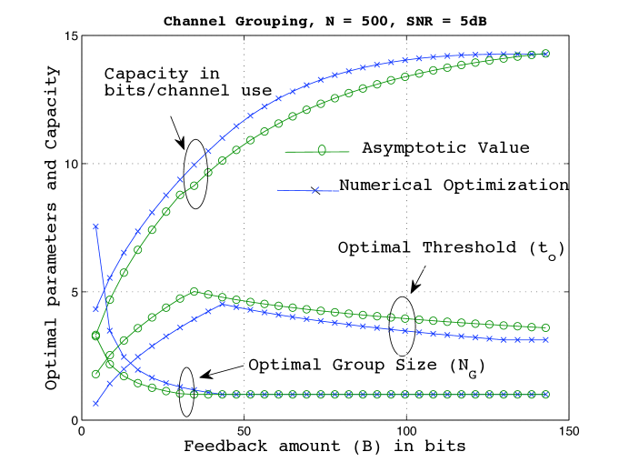
Figure 7: Comparison of numerically optimized values and asymptotic values versus feedback per coherence block for $N=500$ and $P=5$ dB SNR. For comparison, the water-filling capacity is 14.93 bits per channel use.

The preceding asymptotic results are illustrated in Fig. 7. The optimized group size, threshold, and corresponding capacity are plotted as function of the amount of feedback. These results are obtained by optimizing the original capacity expression (31) subject to the feedback constraint. Fig. 7 also shows the asymptotic analytical results. (The values plotted here are refined versions of the expressions presented in Proposition 5 and are derived in Appendix D.) The plot shows that the asymptotic values are close to the values obtained from numerical optimization. As predicted by Proposition 5, the plot shows that as $B$ increases from zero, the group size decreases, and the threshold increases. However, once the group size crosses one (when $B$ is about 40 bits/coherence block), the threshold decreases with $B$ and the capacity increases relatively slowly. Finally, for large amounts of feedback (say, greater than 135 bits/coherence block for this example) the capacity and threshold saturate, and increasing the feedback further does not improve performance. Referring to (79)-(83), these values correspond to $\eta_{1}\approx\eta_{2}\approx 0.25$.

IV-D4 Performance comparison

The optimized forward rate (31) versus $B$ for the group-based scheme is shown in Fig. 4. At 20 dB SNR, grouping sub-channels can provide about $15\%$ gain over threshold adjustment alone for small to moderate feedback rates. As the feedback increases, the two scheme become the same (since the group size converges to $m=1$ at around $B\approx 340$ bits). Recall that the advantage of the group-based scheme over threshold adjustment alone is limited to the feedback range of $B\leq(P/u^{\star})(\log N)^{2-\eta_{1}}$. The optimal threshold for the group-based scheme is shown in Fig. 5. Observe that the optimal thresholds with and without grouping converge for $B\geq 340$. The thresholds behave in strikingly different manners for the two schemes when feedback is smaller.

It is also seen in Fig. 4 that the VQ scheme performs substantially better than both LSC schemes with and without grouping for small to moderate amounts of feedback. Namely, VQ saves between 100 and 150 feedback bits per coherence block over a wide range of target forward rates.

IV-E Growth in achievable forward rate

In this section we highlight several common features of all three schemes discussed in Section IV. With sufficient amount of feedback, all three schemes correspond to the optimal “on-off” power allocation in which the power is uniformly spread over active channels [24, 2]. The optimal threshold is given by

$$t^{\star}=\left[\log N-(1+\eta_{2})\log\log N-\log P\right]+o(1)$$ (33)

and the corresponding capacity is given by (32) for $B\geq B_{max}$ (see Appendix D).

From (83) in Appendix D, as $N\to\infty$, $\eta_{2}\to 1$, so that (32) states that $O(\log^{3}N)$ feedback can achieve the optimal $O(\log N)$ growth in achievable rate. This result has been previously presented in [2], which considers the same threshold-based feedback scheme considered here without grouping ($m=1$). Also, the numerical examples given in the previous section show that for reasonable values of $N$, the amount of feedback needed to achieve the $O(P\log N)$ forward rate may be closer to $P\log^{2}N$ than to $P\log^{3}N$.

At the other extreme of small feedback $B\to 0$, the three schemes also perform similarly and the forward rate converges to the SNR $P$ (see Fig. 4). This limit is the ergodic capacity of a Rayleigh fading channel without feedback when the bandwidth becomes large, i.e., $N\to\infty$. For the VQ scheme, as $B\to 0$, the optimal parameters converge to either $t\to 0,\epsilon_{0}\to 0$, or $t\to\infty,\epsilon_{1}\to 1$, both of which imply the same transmission strategy. Clearly, for threshold adjustment without grouping, the optimal threshold $t^{\star}\to 0$ as feedback becomes small. Finally, although Proposition 5 does not cover the case of finite $B$, it is easy to show that for the group-based scheme, as the amount of feedback $B\to 0$, we have $m\to N$, $t\to 0$ and the achievable rate $C\to P$.

V Correlated Rayleigh fading sub-channels

In this section, we remove the assumption that the Rayleigh fading sub-channels are independent. Suppose the sequence of complex sub-channel coefficients is a Gauss-Markov process generated by the following first-order autoregressive model,

$$H_{i}=\alpha H_{i-1}+\sqrt{1-\alpha^{2}}\,W_{i},\qquad i=2,\ldots,N,$$ (34)

where $W_{i}$ are i.i.d. zero-mean CSCG random variables with unit variance, and $\alpha\in(0,1)$ represents the correlation between the sub-channels. Each sub-channel gain $|H_{i}|^{2}$ is exponentially distributed. The sequence of sub-channel gains $\{|H_{i}|^{2}\}$ is a Markov process with joint second order probability density function given by

$$g(x,y)=\frac{1}{1-\alpha^{2}}e^{-\frac{x+y}{1-\alpha^{2}}}I_{0}\left(\frac{2\alpha\sqrt{xy}}{1-\alpha^{2}}\right)$$ (35)

where $I_{0}(\cdot)$ is the modified Bessel function of the first kind and zero-order.

Again, given a threshold $t\geq 0$, the state vector ${\boldsymbol{S}}$ is defined such that $S_{i}=1$ if $|H_{i}|^{2}\geq t$ and $S_{i}=0$ otherwise. Also, $q={\mathsf{P}}\left\{S_{i}=1\right\}=e^{-t}$. The sequence $\{S_{i}\}$ is a hidden Markov process rather than i.i.d. Nonetheless, for a fixed $p$ and $t$, the rate-distortion trade-off is still given by (16). However, obtaining upper and lower bounds on the required feedback rate (16), analogous to the two state Markov model of Section III, seems to be difficult due to the hidden Markov structure of ${\boldsymbol{S}}$.

We proceed by assuming that the receiver approximates the sequence $\{S_{i}\}$ as a first-order Markov chain. Ignoring the higher order correlation in ${\boldsymbol{S}}$ results in a larger feedback requirement (or equivalently, an upper bound on $R(D)$ in (16)). Using this upper bound as the feedback rate then gives an achievable forward rate (a lower bound on capacity). The transition probabilities for the first-order Markov model are,

$$\delta_{10} =\Pr\{S_{i}=0|S_{i\pm 1}=1\}=1-\frac{1}{q}\int_{t}^{\infty}\int_{t}^{\infty}g(x,y)\text{d}x\text{d}y,$$ (36)

$$\delta_{01} =\Pr\{S_{i}=1|S_{i\pm 1}=0\}=\frac{q\delta_{10}}{1-q}\,.$$ (37)

With the first-order Markov approximation, the problem reduces to the one discussed in Section III. Consequently, an achievable forward rate can be computed by solving the optimization problem (29) over $p,t,\epsilon_{0}$ and $\epsilon_{1}$ with $q=e^{-t}$ and the constraint (10b) replaced by $i_{u}(\epsilon_{0},\epsilon_{1})\leq R_{f}$. An expression for $i_{u}(\epsilon_{0},\epsilon_{1})$ is given in Appendix C.

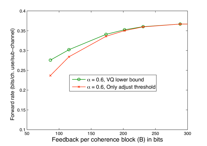
Figure 8: Achievable forward rate versus the feedback rate for a VQ scheme with correlated fading sub-channels. Also shown is the forward rate achieved with the threshold adjustment feedback scheme without grouping. Other parameters are $N=500$, $P=20$ dB SNR. For comparison, the water-filling capacity with full channel state information at receiver is 0.385 bits per sub-channel use (the same as in Fig. 4).

Fig. 8 plots this rate versus feedback per coherence block $B=NR_{f}$ for $\alpha=0.6$ and 20 dB SNR. Also shown in Fig. 8 is the forward rate achieved with the simpler LSC feedback scheme that encodes the state vector ${\boldsymbol{S}}$ and controls the amount of feedback by adjusting the threshold without grouping. Allowing no errors in the reconstructed channel state vector means that the minimum required feedback rate is $H({\boldsymbol{S}})$, which is upper bounded by $H(S_{1}|S_{0})=qH_{2}(\delta_{10})+(1-q)H_{2}(\delta_{01})$. This feedback scheme was considered for correlated sub-channels in [24]. In Fig. 8, VQ performs substantially better at small to moderate feedback rates. The forward rate values were also computed for $\alpha=0.9$ (not shown in Fig. 8), but there the comparison is inconclusive, since the lower bound on forward rate achieved with VQ is very close to the forward rate achieved with the LSC scheme.

The behavior of the optimal threshold and crossover probabilities $\epsilon_{0},\epsilon_{1}$ is the same as for independent sub-channels and hence is not shown here. Similar to the independent sub-channels case, we can again apply the group-based scheme to correlated sub-channels. Performance evaluation appears to be difficult, but the performance of the group-based scheme should be inferior to that of the VQ scheme and at least as good than without grouping.

VI Conclusions

We have studied limited feedback of channel states for multicarrier systems with two-state and Rayleigh sub-channels. The asymptotic performance has been characterized, using rate distortion theory, along with bounds on the performance loss with a finite number of sub-channels. For Rayleigh channels, the threshold-based VQ scheme shows a substantial improvement over lossless coding of reduced channel states based on thresholding, especially at low to moderate SNRs. Of course, this benefit comes at the price of higher source coding complexity (e.g., using graphical codes).

Our results have assumed perfect channel knowledge at the receiver and have neglected the feedback overhead. In practice, the combined overhead for channel estimation and feedback compromises the benefits of feedback. This becomes more important as the channel coherence time decreases. A model, which accounts for feedback overhead in a multicarrier time-division duplex system is presented in [25]. There the overhead is optimized, assuming the lossless feedback code presented in Section IV-D. Training and feedback overhead in the context of beamforming has been studied in [26, 27]. That approach may also be appropriate for the multicarrier scenario considered here.

We have also assumed a noiseless feedback link. For the schemes considered here a noisy feedback link requires additional overhead in the form of channel coding or higher transmit power. Other alternatives include analog CSF (e.g., see [28, 29]), which gives noisy estimates at the transmitter, and sending a pilot signal from receiver to transmitter at the beginning of each coherence block[30] (assuming channel reciprocity applies). Comparative advantages and disadvantages of these schemes remain to be studied.

Finally, the results presented here can conceivably be extended to more elaborate system and channel models, such as continuous fading, instead of block fading (e.g., see [31, 32]), and Multiple-Input Multiple-Output (MIMO) OFDM. Such systems typically operate at low SNRs per antenna (or coefficient) and hence can benefit substantially from adaptive power loading[33, 34]. Limited CSF schemes for downlink and uplink OFDMA are presented in [35, 23, 36] and the references therein. (See also the comprehensive survey of the limited feedback literature in [37].) Extensions of the VQ scheme presented here to those settings is also left for future work.

Appendix A Proof of Proposition 2

First we introduce some notation, then describe the construction of a fixed-length, constant-composition feedback code, and finally give the performance bounds as a function of $N$.

Let $\mathcal{P}_{{\boldsymbol{s}}}(1)$ represent the empirical probability of ones in a length $N$ binary vector channel state ${\boldsymbol{s}}$. Namely, $\mathcal{P}_{{\boldsymbol{s}}}(1)=q$ implies that $\sum_{i=1}^{N}s_{i}=qN$. A similar definition holds for $\mathcal{P}_{\hat{{\boldsymbol{s}}}}(1)$. Furthermore, for any pair of vectors $(\hat{{\boldsymbol{s}}},{\boldsymbol{s}})$, $\mathcal{P}_{\hat{{\boldsymbol{s}}}|{\boldsymbol{s}}}(0|1)$ represents the empirical probability of zeroes in $\hat{{\boldsymbol{s}}}$ at the positions where ${\boldsymbol{s}}$ has ones. In other words, $\mathcal{P}_{\hat{{\boldsymbol{s}}}|{\boldsymbol{s}}}(0|1)=\epsilon_{0}$ implies that $\sum_{i=1}^{N}1_{\{\hat{s}_{i}=0,s_{i}=1\}}=\epsilon_{0}\mathcal{P}_{{\boldsymbol{s}}}(1)N$. Let $\mathbf{\mathcal{T}}_{{\boldsymbol{S}};q}$ represent the set of all constant composition length $N$ channel state vectors ${\boldsymbol{s}}$ which have $qN$ number of ones, that is, $\mathbf{\mathcal{T}}_{{\boldsymbol{S}};q}=\{{\boldsymbol{s}}:\mathcal{P}_{{\boldsymbol{s}}}(1)=q\}$. Similarly, define the set of constant composition power loading vectors $\mathbf{\mathcal{T}}_{\hat{{\boldsymbol{S}}};p}=\{\hat{{\boldsymbol{s}}}:\mathcal{P}_{\hat{{\boldsymbol{s}}}}(1)=p\}$.

Let the feedback codebook be a subset $\mathbf{\mathcal{T}}_{\hat{{\boldsymbol{S}}}|{\boldsymbol{S}}}\subset\mathbf{\mathcal{T}}_{\hat{{\boldsymbol{S}}};p}$. The amount of feedback required per coherence block is therefore $\log_{2}|\mathbf{\mathcal{T}}_{\hat{{\boldsymbol{S}}}|{\boldsymbol{S}}}|$ bits. A vector ${\boldsymbol{s}}\in\mathbf{\mathcal{T}}_{\hat{{\boldsymbol{S}}}|{\boldsymbol{S}}}$ is said to cover ${\boldsymbol{s}}\in\mathbf{\mathcal{T}}_{{\boldsymbol{S}};q}$ if $\mathcal{P}_{\hat{{\boldsymbol{s}}}|{\boldsymbol{s}}}(0|1)=\epsilon_{0}$ and $\mathcal{P}_{\hat{{\boldsymbol{s}}}|{\boldsymbol{s}}}(1|0)=\epsilon_{1}$. Note that depending on the size of the codebook, all the vectors in $\mathbf{\mathcal{T}}_{{\boldsymbol{S}};q}$ might not be covered. The feedback occurs as follows: Every channel realization vector is matched to the closest (in hamming distance) typical vector ${\boldsymbol{s}}\in\mathbf{\mathcal{T}}_{{\boldsymbol{S}};q}$. The receiver then looks up a $\hat{{\boldsymbol{s}}}$ in $\mathbf{\mathcal{T}}_{\hat{{\boldsymbol{S}}}|{\boldsymbol{S}}}$ which covers ${\boldsymbol{s}}$ feeds back the index of $\hat{{\boldsymbol{s}}}$. If there is no such $\hat{{\boldsymbol{s}}}$ then a random index is fed back. Therefore, the elements of the codebook $\mathbf{\mathcal{T}}_{\hat{{\boldsymbol{S}}}|{\boldsymbol{S}}}$ should be chosen carefully to minimize the distortion or, equivalently, maximize the forward rate. Next, along the lines of [11], we will evaluate the average performance assuming that the subset $\mathbf{\mathcal{T}}_{\hat{{\boldsymbol{S}}}|{\boldsymbol{S}}}$ is chosen at random. Then by usual argument we can claim that there must exist a structured fixed-length constant composition codebook that does at least as well.

Consider the performance of the codebook as a function of $N$. The Type covering lemma [38] suggests that we can find a codebook with size $|\mathbf{\mathcal{T}}_{\hat{{\boldsymbol{S}}}|{\boldsymbol{S}}}|=g(N)2^{i(\epsilon_{0},\epsilon_{1})N}$, where $g(N)$ is a polynomial, such that every vector in $\mathbf{\mathcal{T}}_{{\boldsymbol{S}};q}$ is covered. Here, we use random coding arguments to get an estimate of $g(N)$. Suppose $\mathbf{\mathcal{T}}_{\hat{{\boldsymbol{S}}}|{\boldsymbol{S}}}$ consists of $M$ vectors that are randomly and independently drawn from $\mathbf{\mathcal{T}}_{\hat{{\boldsymbol{S}}};p}$.

Given a vector ${\boldsymbol{s}}\in\mathbf{\mathcal{T}}_{{\boldsymbol{S}};q}$, probability that it will be not be covered by the $M$ randomly chosen vectors is given by

$$p_{n} =[1-p_{c}]^{M}\leq e^{-Mp_{c}}$$ (38)

where

$$p_{c}=\frac{{qN\choose\epsilon_{0}qN}{(1-q)N\choose\epsilon_{1}(1-q)N}}{{N\choose pN}}.$$ (39)

Further using Robbin’s approximation [39, 38] for the factorial

$$\sqrt{2\pi}\,n^{n+\frac{1}{2}}e^{-n+\frac{1}{12(n+1)}}\leq n!\leq\sqrt{2\pi}\,n^{n+\frac{1}{2}}e^{-n+\frac{1}{12n}},\qquad n\geq 1,$$ (40)

it is straightforward to show that

$$p_{c}\geq N^{-1/2}2^{-K_{2}}\,2^{-i(\epsilon_{0},\epsilon_{1})N}$$ (41)

where the mutual information $i(\epsilon_{0},\epsilon_{1})$ is given by (8) and $K_{2}=\log_{2}(\sqrt{2\pi}e^{5/12})-\frac{1}{2}\log_{2}(p(1-p))$ is a constant. Now choosing $M=(\log N)N^{1/2}2^{K_{2}}\,2^{i(\epsilon_{0},\epsilon_{1})N}$ and combining (38) and (41) gives $p_{n}\leq 1/N$. Therefore, with this codebook the feedback rate per sub-channel per coherence block given by

$$\frac{\log_{2}|\mathbf{\mathcal{T}}_{\hat{{\boldsymbol{S}}}|{\boldsymbol{S}}}|}{N}=\frac{\log_{2}M}{N}=i(\epsilon_{0},\epsilon_{1})+\frac{(\log_{2}N+2K_{2}+2\log_{2}(\log N))}{2N}$$ (42)

converges to the mutual information $i(\epsilon_{0},\epsilon_{1})$.

Next we bound the average forward rate achieved by this codebook. For this we need to account for the variations in the channel gain vector ${\boldsymbol{S}}$. Consider the set of channel gain vectors with fraction of ones in the range $(q(1-\epsilon),q(1+\epsilon))$, that is, say $\mathbf{\mathcal{T}}_{{\boldsymbol{S}};q}^{\epsilon}=\{{\boldsymbol{s}}:\mathcal{P}_{\boldsymbol{s}}(1)\in(q(1-\epsilon),q(1+\epsilon))\}$. Using Chernoff’s inequality [40], the following is easily seen

$$\Pr\bigg{\{}\bigg{|}\sum_{i=1}^{N}S_{i}-qN\bigg{|}\geq q\epsilon N\bigg{\}}\leq p_{u}=2\exp\left(-\frac{qN\epsilon^{2}}{4}\right),\qquad 0\leq\epsilon\leq 2(1-q),$$ (43)

which in turn implies that $\Pr\{\mathbf{\mathcal{T}}_{{\boldsymbol{S}};q}^{\epsilon}\}\geq 1-p_{u}$. Using the definition of $\epsilon$ above, the ergodic capacity is lower bounded as

$$C_{fixed} \geq q(1-\epsilon_{0}-\epsilon)(C_{1}-C_{0})\left(1-p_{u}\right)(1-p_{n})+pC_{0}$$ (44)

$$\geq C-C\left(\epsilon+p_{u}+\frac{1}{N}\right),$$ (45)

where $C=q(1-\epsilon_{0})(C_{1}-C_{0})+pC_{0}$. The loss factors $1-p_{n}$ and $1-p_{u}$ in (44) account for the fact that channel gain vectors might not be covered or, might not be in the set $\mathbf{\mathcal{T}}_{{\boldsymbol{S}};q}^{\epsilon}$, respectively. Further, choosing $\epsilon=\sqrt{\frac{2\log(Nq)}{Nq}}$ gives a tight lower bound as

$$C_{fixed}\geq C-C\left(\frac{\sqrt{2\log(Nq)}+2}{\sqrt{Nq}}+\frac{1}{N}\right)\ .$$ (46)

In summary, since (46) bounds the average performance of a randomly generated codebook with $M$ codewords, there must exist a codebook of size $M$ which performs at least as good as this lower bound.

Lastly, we consider the convergence rate to the upper bound given by Proposition 1. Note that required feedback rate (42) is more than mutual information $i(\epsilon_{0},\epsilon_{1})$. If we do not wish to allow the feedback to exceed $i(\epsilon_{0},\epsilon_{1})$ bits per sub-channel, an additional distortion of $\delta$ can be introduced so that $\epsilon_{0}$ and $\epsilon_{1}$ are replaced by $\epsilon_{0}+\delta$ and $\epsilon_{1}+\delta^{\prime}$, respectively, where $\delta^{\prime}={q\delta}/(1-q)$ (so that the input power constraint (10c) is satisfied). Using Taylor series expansion, for a small enough $\delta$ we have

$$-2q[H_{2}^{\prime}(\epsilon_{0})+H_{2}^{\prime}(\epsilon_{1})]\delta\leq i(\epsilon_{0}+\delta,\epsilon_{1}+\delta^{\prime})-i(\epsilon_{0},\epsilon_{1})\leq-\frac{1}{2}q[H_{2}^{\prime}(\epsilon_{0})+H_{2}^{\prime}(\epsilon_{1})]\delta.$$ (47)

Substituting $\epsilon_{0}+\delta$ and $\epsilon_{1}+\delta^{\prime}$ for $\epsilon_{0}$ and $\epsilon_{1}$ in (42) and using (47), for large enough $N$ and small enough $\delta$ we have

$$\frac{\log_{2}|\mathbf{\mathcal{T}}_{\hat{{\boldsymbol{S}}}|{\boldsymbol{S}}}|}{N}\leq i(\epsilon_{0},\epsilon_{1})-\frac{1}{2}q[H_{2}^{\prime}(\epsilon_{0})+H_{2}^{\prime}(\epsilon_{1})]\delta+\frac{\log_{2}N}{N}\ .$$ (48)

Now choosing $\delta=K_{1}\frac{\log_{2}N}{N}$ where $K_{1}=\frac{2}{q[H_{2}^{\prime}(\epsilon_{0})+H_{2}^{\prime}(\epsilon_{1})]}$, gives that the number of feedback bits per sub-channels $\frac{\log_{2}|\mathbf{\mathcal{T}}_{\hat{{\boldsymbol{S}}}|{\boldsymbol{S}}}|}{N}\leq i(\epsilon_{0},\epsilon_{1})$. The additional distortion of $\delta$ will result in a loss in capacity which can be quantified by replacing $\epsilon_{0}$ by $\epsilon_{0}+\delta$ in (44) which gives a lower bound on forward rate as

$$C_{fixed}\geq C-C\left(\frac{\sqrt{2\log(Nq)}+2}{\sqrt{Nq}}+\frac{1}{N}+K_{1}\frac{\log_{2}N}{N}\right)$$ (49)

which for large enough $N$ can be further lower bounded as (12).

Appendix B Proof of Proposition 3

We again resort to the random coding techniques as in [12], assuming that corresponding to each channel state vector ${\boldsymbol{s}}$, the power loading vector $\hat{{\boldsymbol{s}}}$ is produced with Bernoulli-$p$ distribution. A randomly generated codeword $\hat{{\boldsymbol{s}}}$ is admitted only if it satisfies the empirical probabilities $\mathcal{P}_{\hat{{\boldsymbol{s}}}|{\boldsymbol{s}}}(0|1)=\epsilon_{0}$ and $\mathcal{P}_{\hat{{\boldsymbol{s}}}|{\boldsymbol{s}}}(1|0)=\epsilon_{1}$, where $\epsilon_{0}$ and $\epsilon_{1}$ are fixed and $q(1-\epsilon_{0})+(1-q)\epsilon_{1}=p$. This will ensure that averaged over all the state vectors, the number of sub-channels used for transmission are given by $pN$ and average number of unused good sub-channels are $q\epsilon_{0}N$. Next, we shall find the expected variable-length encoder rate, averaged over this ensemble of codes, and then, by usual argument, we can assert that there must exist at least one set of $\{\hat{{\boldsymbol{s}}}\}$ that gives the performance as good as the average.

Let $L$ represent the random variable denoting the fraction of ones in the state vector ${\boldsymbol{S}}$. Clearly, $H(L)\leq\log_{2}(N+1)$. If a variable-length feedback codebook with average rate of $R_{f}$ bits per sub-channel per coherence block is used, then we can write $NR_{f}\leq H(\hat{{\boldsymbol{S}}})+1$. The rate can be further upper bounded as $NR_{f}\leq H(\hat{{\boldsymbol{S}}},L)+1=H(\hat{{\boldsymbol{S}}}|L)+H(L)+1$. Averaging over the random code book selection we get that,

$$NR_{f}\leq E_{\hat{{\boldsymbol{S}}}}[H(\hat{{\boldsymbol{S}}}|L)]+H(L)+1.$$ (50)

Corresponding to a channel state vector with $L=l$, define $q_{l}$ as the probability that a randomly drawn codeword $\hat{{\boldsymbol{s}}}$ is admissible. Then we have,

$$q_{l}={lN\choose\epsilon_{0}lN}{(1-l)N\choose\epsilon_{1}(1-l)N}\,p^{n(l)N}(1-p)^{(1-n(l))N},$$ (51)

where $n(l)=(1-\epsilon_{0})l+\epsilon_{1}(1-l)$. Further, it is argued in [12] that given the geometric distribution $p(k|l)=q_{l}(1-q_{l})^{k-1}$ we have

$$E_{\hat{{\boldsymbol{S}}}}[H(\hat{{\boldsymbol{S}}}|l)] =-\sum_{k=1}^{\infty}p(k|l)\log_{2}p(k|l)$$ (52)

$$\leq-\log_{2}q_{l}+\log_{2}e.$$ (53)

Combining (50) and (53) and using the fact that $H(L)\leq\log_{2}(N+1)$ we have,

$$NR_{f}\leq-\sum_{l=0}^{N}(\log_{2}q_{l})\Pr\{L=l\}+\log_{2}e+\log_{2}(N+1)+1.$$ (54)

Further, applying Robbin’s approximation (40) to (51) we have

$$\begin{split}-\log_{2}(q_{l})\leq-lNH_{2}(\epsilon_{0})&-(1-l)NH_{2}(\epsilon_{1})\\ +&n(l)N\log_{2}(p)+(1-n(l))N\log_{2}(1-p)+\log_{2}N+K_{3},\end{split}$$ (55)

where $K_{3}=\frac{1}{2}\log_{2}[e^{8}(2\pi)^{2}\epsilon_{0}\epsilon_{1}(1-\epsilon_{0})(1-\epsilon_{1})]$. Substituting (55) into (54) and using the fact that $E[n(l)]=p$ and $E[l]=q$, we get,

$$R_{f}\leq i(\epsilon_{0},\epsilon_{1})+\frac{1}{N}(\log_{2}e+K_{3}+\log_{2}N+\log_{2}(N+1)+1)\ .$$ (56)

Since this rate exceeds $i(\epsilon_{0},\epsilon_{1})$, similar to Appendix A, we can introduce additional distortion so that $\epsilon_{0}$ and $\epsilon_{1}$ are replaced by $\epsilon_{0}+\delta$ and $\epsilon_{1}+\frac{q\delta}{1-q}$. Therefore, using (47), for large enough $N$ and small enough $\delta$, (56) yields

$$R_{f}\leq i(\epsilon_{0},\epsilon_{1})-\frac{1}{2}q[H_{2}^{\prime}(\epsilon_{0})+H_{2}^{\prime}(\epsilon_{1})]\delta+\frac{3\log_{2}N}{N}$$ (57)

Finally, choosing $\delta=\frac{6\log_{2}N}{q[H_{2}^{\prime}(\epsilon_{0})+H_{2}^{\prime}(\epsilon_{1})]N}$ gives $R_{f}\leq i(\epsilon_{0},\epsilon_{1})$ and capacity as (13).

Appendix C Derivation of $i_{l}(q_{00},q_{01},q_{10},q_{11})$ and $i_{u}(\epsilon_{0},\epsilon_{1})$

The lower bound can be explicitly computed as follows

$$i_{l}(q_{00},q_{01},q_{10},q_{11}) =I(S_{1};\hat{S}_{1}|S_{0})$$ (58)

$$=H(\hat{S}_{1}|S_{0})-H(\hat{S}_{1}|S_{1},S_{0}).$$ (59)

Each entropy term is further computed as

$$H(\hat{S}_{1}|S_{0})=(1-q)H_{2}\left(\frac{q_{00}+q_{01}}{1-q}\right)+qH_{2}\left(\frac{q_{10}+q_{11}}{q}\right)$$ (60)

and

$$\begin{split}H(\hat{S}_{1}|S_{1},S_{0})=(1-q)&(1-\delta_{01})H_{2}\left(\frac{q_{00}}{(1-q)(1-\delta_{01})}\right)+q\delta_{10}H_{2}\left(\frac{q_{10}}{q\delta_{10}}\right)\\ &+(1-q)\delta_{01}H_{2}\left(\frac{q_{01}}{(1-q)\delta_{01}}\right)+q(1-\delta_{10})H_{2}\left(\frac{q_{11}}{q(1-\delta_{10})}\right).\end{split}$$ (61)

Next we compute the upper bound $f_{2}(\epsilon_{0},\epsilon_{1})$. Recall that, in order to arrive at the upper bound, we have assumed that conditioned on $S_{i}$, $\hat{S}_{i}$ is independent of all other elements in ${\boldsymbol{S}}$, thus

$$i_{u}(\epsilon_{0},\epsilon_{1}) =I(S_{1};S_{2},\hat{S}_{1}|S_{0})$$ (62)

$$=H(S_{2},\hat{S}_{1}|S_{0})-H(S_{2},\hat{S}_{1}|S_{1},S_{0})$$ (63)

$$=H(S_{2}|S_{0})+H(\hat{S}_{1}|S_{0},S_{2})-H(\hat{S}_{1}|S_{1})-H(S_{2}|S_{1}).$$ (64)

Each entropy term can be further computed as

$$H(S_{2}|S_{0}) =qH_{2}\left((1-\delta_{10})^{2}+\delta_{10}\delta_{01}\right)+(1-q)H_{2}\left(\delta_{01}(1-\delta_{10})+(1-\delta_{01})\delta_{01}\right),$$ (65)

$$H(\hat{S}_{1}|S_{1}) =qH_{2}(\epsilon_{0})+(1-q)H_{2}(\epsilon_{1}),$$ (66)

$$H(S_{2}|S_{1}) =qH_{2}(\delta_{10})+(1-q)H_{2}(\delta_{01})$$ (67)

and

$$\begin{split}H(\hat{S}_{1}|S_{0},S_{2})=&\left((1-\delta_{01})^{2}(1-q)+\delta_{10}^{2}q\right)H_{2}\left(w_{00}\right)\\ &\qquad+2\left(\delta_{01}(1-\delta_{01})(1-q)+\delta_{10}(1-\delta_{10})q\right)H_{2}\left(w_{01}\right)\\ &\qquad\qquad+\left(\delta_{01}^{2}(1-q)+(1-\delta_{10})^{2}q\right)H_{2}\left(w_{11}\right),\end{split}$$ (68)

where the probabilities in the argument of binary entropy functions are defined as,

$$w_{s_{0}s_{2}}=P_{\hat{S}_{1}|S_{0},S_{2}}(0|s_{0},s_{2}),\quad s_{0},s_{2}=0\text{ or }1.$$ (69)

We note that $w_{10}=w_{01}$ and the probabilities can be explicitly computed as

$$w_{00} =\frac{(1-\epsilon_{1})(1-\delta_{01})^{2}(1-q)+\epsilon_{0}\delta_{10}^{2}q}{(1-\delta_{01})^{2}(1-q)+\delta_{10}^{2}q},$$ (70)

$$w_{01} =\frac{(1-\epsilon_{1})\delta_{01}(1-\delta_{01})(1-q)+\epsilon_{0}\delta_{10}(1-\delta_{10})q}{\delta_{01}(1-\delta_{01})(1-q)+\delta_{10}(1-\delta_{10})q},$$ (71)

$$w_{11} =\frac{(1-\epsilon_{1})\delta_{01}^{2}(1-q)+\epsilon_{0}(1-\delta_{10})^{2}q}{\delta_{01}^{2}(1-q)+(1-\delta_{10})^{2}q}\ .$$ (72)

Appendix D Proof Sketch of Proposition 5

Consider the maximization of the capacity $C(m,t)$ in (31) over the group size $m$ and threshold $t$ subject to $GH(q)\leq B$. The capacity can be bounded as

$$Nq\log\left(1+\frac{Pt}{Nq}\right)\leq C(m,t)\leq Nq\log\left(1+\frac{P(t+1)}{Nq}\right).$$ (73)

The lower bound is simply by observing that the logarithm term in (31) takes on its minimum value at the boundary $\tau=t$, whereas the exponential term integrates to 1. The upper bound can be shown using the fact that $\int_{0}^{\infty}e^{-x}\log(x+a)\,\text{d}\tau<\log(1+a)$ for all $a>0$. Clearly, the maximum value of $C(m,t)$ subject to $GH(q)\leq B$ is no greater than the maximum value of the upper bound of $C(m,t)$ in (73) subject to the same constraint. Next we obtain a solution to the latter optimization problem and show that for large $B$ and $N$, it provides a good approximation to the solution of the original optimization problem. Without loss of generality, substituting $w=Nq$ the optimization problem can be written as

$$\max_{w,t}\,\,\bar{C}=w\log\left(1+\frac{P(t+1)}{w}\right),\,\,\textrm{subject to:}\,\,w\,t\leq B.$$ (74)

Assuming that the feedback constraint is tight, i.e., $w\,t=B$, the optimum $w$ must satisfy

$$(1+u+P/w)\log(1+u+P/w)=(1+2u+P/w),$$ (75)

where $u=PB/{w^{2}}$. A closed-form solution to (75) seems difficult, however, insight can be obtained by assuming that $N,B$ are large. In addition, we assume that the optimal $w$ increases with $B$ such that $u\gg P/w$ or, equivalently, as $B\to\infty$, $w/B\to 0$. We will see later that this is indeed true. Therefore, observing that the $P/w$ terms in (75) are small compared to $u$, the optimal $w^{\star}=\sqrt{\frac{PB}{u^{\star}}}+o(1)$, where $o(1)$ is vanishingly small as $B\to\infty$, and $u^{\star}$ is the solution to $(1+u^{\star})\log(1+u^{\star})=(1+2u^{\star})$. Since we assume that $wt=B$, solving (74) gives

$$t^{\star} =\sqrt{\frac{u^{\star}B}{P}}+o(1)$$ (76)

$$m^{\star} =\sqrt{\frac{P}{u^{\star}B}}\log\frac{N}{\sqrt{P\,B/u^{\star}}}+o(1)$$ (77)

$$\bar{C} =\sqrt{\frac{PB}{u^{\star}}}\log(1+u^{\star})+o(1).$$ (78)

The parameter values satisfy the original feedback constraint $GH(q)=B$ and in fact the lower bound in (73) also behaves as (78) (although the value associated with the $o(1)$ term change). This implies that the optimal parameters that maximize the capacity $C(m,t)$ satisfy (76) and (77), and the capacity $C^{\star}$ is approximated by (78) to within a vanishingly small term.

Note that (77) implies that for $m^{\star}>1$ we should have feedback in the range $B<\frac{P}{u^{\star}}(\log N)^{2-\eta_{1}}$ for large $N$ where $\eta_{1}\in(0,2)$ is the solution to

$$\log N-\log\left[\frac{P}{u^{\star}}(\log N)^{1-\frac{\eta_{1}}{2}}\right]=(\log N)^{1-\frac{\eta_{1}}{2}}.$$ (79)

It is easy to see that $\eta_{1}\to 0$ as $N\to\infty$. Next we solve for the optimal parameters when $B\geq\frac{P}{u^{\star}}(\log N)^{2-\eta_{1}}$. Again we first solve the upper bound maximization problem (74) with $m=1$ or, equivalently $q=e^{-t}$. Namely

$$\max_{t}\,\bar{C}=Ne^{-t}\log\left(1+\frac{P(t+1)}{Ne^{-t}}\right),\,\,\textrm{subject to:}\,\,Nte^{-t}\leq B.$$ (80)

Assuming that the feedback constraint is tight, i.e., $Nte^{-t}=B$, we get the optimal threshold and upper bound on capacity

$$t^{\star} =\log\frac{N\log N}{B}+o(1)$$ (81)

$$\bar{C} =\frac{B}{\log N}\log\left(1+\frac{P\log N}{B}\log\frac{N\log N}{B}\right)+O(1)$$ (82)

Again, it can be checked that with appropriate adjustments to the $o(1)$ and $O(1)$ terms in (81) and (82), respectively, the threshold (81) satisfies the original feedback constraint $NH(e^{-t})=B$ and the lower bound in (73) also behaves as (82). This implies that the threshold, which maximizes the capacity $C$ in the feedback range $B\geq\frac{P}{u^{\star}}(\log N)^{2-\eta_{1}}$ satisfies (81), $m^{\star}=1$ and the capacity $C^{\star}$ is also given by (82).

Furthermore, note that as $B$ increases, the threshold (81) decreases. However, decreasing the threshold beyond a certain optimal value decreases the capacity upper bound in (80). The optimum value of the threshold that maximizes the upper bound in (80) is given by (33) and the corresponding upper bound is given in (32), corresponding to $B>B_{max}$, where $\eta_{2}\in(0,1)$ is the solution to

$$\log N-\log[P(\log N)^{1+\eta_{2}}]=(\log N)^{(1+\eta_{2})/2}.$$ (83)

Clearly, $\eta_{2}\to 1$ as $N\to\infty$. Substituting $m=1$ and (33) into the lower bound in (73) gives that the lower bound and hence the capacity also behave as in (32). Therefore, the optimal threshold that maximizes the capacity is given by (33) with adjusted $o(1)$ term. Corresponding to (33), the maximum required feedback is given by $B_{max}=NH(e^{-t})=P(\log N)^{2+\eta_{2}}+o(\log^{2}N)$.

References

- [1] D. N. C. Tse and P. Viswanath, Fundamentals of Wireless Communication. Cambridge University Press, 2005.
- [2] Y. Sun and M. L. Honig, “Asymptotic capacity of multicarrier transmission with frequency-selective fading and limited feedback,” IEEE Trans. Inform. Theory, vol. 54, no. 7, pp. 2879–2902, July 2008.
- [3] S. Sanayei and A. Nosratinia, “Opportunistic downlink transmission with limited feedback,” IEEE Trans. Inform. Theory, vol. 53, no. 11, pp. 4363–4372, Nov. 2007.
- [4] D. Love and R. W. Heath Jr., “OFDM power loading using limited feedback,” IEEE Trans. Veh. Technol., vol. 54, no. 5, pp. 1773–1780, Sept. 2005.
- [5] Y. Rong, S. A. Vorobyov, and A. B. Gershman, “Adaptive OFDM techniques with one-bit-per-subcarrier channel-state feedback,” IEEE Trans. Wireless Commun., vol. 54, no. 11, Nov. 2006.
- [6] Y. Sun and M. Honig, “Minimum feedback rates for multicarrier transmission with correlated frequency-selective fading,” Proc. IEEE GLOBECOM, vol. 3, pp. 1628–1632, Dec. 2003.
- [7] J. Chen, R. Berry, and M. L. Honig, “Performance of limited feedback schemes for downlink OFDMA with finite coherence time,” in Proc. IEEE Int. Symp. Inform. Theory. Nice, France, Jun. 2007.
- [8] T. Tang, R. W. Heath, S. Cho, and S. Yun, “Opportunistic feedback in clustered OFDM system,” in International Symposium on Wireless Personal Multimedia Communications. San Diego, CA, Sep. 2006.
- [9] L. Cimini Jr., B. Daneshrad, and N. Sollenberger, “Clustered OFDM with transmitter diversity and coding,” Proc. IEEE GLOBECOM, vol. 1, pp. 703–707, Nov 1996.
- [10] T. M. Cover and J. A. Thomas, Elements of Information Theory, 2nd ed. Wiley, 2006.
- [11] T. J. Goblick, “Coding for a discrete information source with a distortion measure,” Ph.D. dissertation, M.I.T., 1962.
- [12] J. T. Pinkston, “Encoding independent sample information sources,” Ph.D. dissertation, M.I.T., 1967.
- [13] V. K. N. Lau, Y. J. Liu, and T.-A. Chen, “Capacity of memoryless channels and block-fading channels with designable cardinality-contrained channel state feedback,” IEEE Trans. Inform. Theory, vol. 50, no. 9, pp. 2038–2049, Sep. 2004.
- [14] V. K. N. Lau, Y. Liu, and T.-A. Chen, “On the design of MIMO block-fading channels with feedback-link capacity constraint,” IEEE Trans. Commun., vol. 52, no. 1, pp. 62–70, Jan. 2004.
- [15] A. Lau and F. Kschischang, “Feedback quantization strategies for multiuser diversity systems,” IEEE Trans. Inform. Theory, vol. 53, no. 4, pp. 1386–1400, April 2007.
- [16] E. Martinian and M. Wainwright, “Low density codes achieve the rate-distortion bound,” Proc. Data Compression Conference, pp. 153–162, March 2006.
- [17] M. Wainwright, “Sparse graph codes for side information and binning,” IEEE Signal Processing Mag., vol. 24, no. 5, pp. 47–57, Sept. 2007.
- [18] G. Caire, S. Shamai, and S. Verdú, “Universal data compression with LDPC codes,” in Third International Symposium On Turbo Codes and Related Topics. Brest, France, Sep. 2003.
- [19] T. Berger, Rate Distortion Theory. Englewood Cliffs, NJ: Prentice-Hall, 1971.
- [20] R. Gray, “Information rates of autoregressive processes,” IEEE Trans. Inform. Theory, vol. 16, no. 4, pp. 412–421, Jul 1970.
- [21] E. Ordentlich and T. Weissman, “New bounds on the entropy rate of hidden Markov processes,” in Proc. IEEE Inform. Theory Workshop. San Antonio, TX, USA, Oct. 2004, pp. 117–122.
- [22] J. Luo and D. Guo, “On the entropy rate of hidden Markov processes observed through arbitrary memoryless channels,” IEEE Trans. Inform. Theory, 2009, to appear.
- [23] J. Chen, R. Berry, and M. Honig, “Limited feedback schemes for downlink OFDMA based on sub-channel groups,” IEEE J. Select. Areas Commun., vol. 26, no. 8, pp. 1451–1461, October 2008.
- [24] Y. Sun and M. Honig, “Minimum feedback rates for multicarrier transmission with correlated frequency-selective fading,” IEEE Global Telecommunications Conference, vol. 3, pp. 1628–1632 vol.3, 1-5 Dec. 2003.
- [25] M. Agarwal, D. Guo, and M. L. Honig, “Multi-carrier transmission with limited feedback: Power loading over sub-channel groups,” in Proc. IEEE Int. Conf. Commun. Beijing, China, 2008, pp. 981–985.
- [26] W. Santipach and M. L. Honig, “Optimization of training and feedback for beamforming over a MIMO channel,” in Proc. IEEE Wireless Commun. and Networking Conf. (WCNC). Hong Kong, China, Mar. 2007.
- [27] M. Kobayashi, G. Caire, N. Jindal, and N. Ravindran, “How much training and feedback are needed in MIMO broadcast channels?” in Proc. IEEE Int. Symp. Inform. Theory. Toronto, Canada, Jul. 2008.
- [28] T. Marzetta and B. Hochwald, “Fast transfer of channel state information in wireless systems,” IEEE Trans. Signal Processing, vol. 54, no. 4, pp. 1268–1278, Apr. 2006.
- [29] G. Caire, N. Jindal, M. Kobayashi, and N. Ravindran, “Multiuser MIMO downlink made practical: Achievable rates with simple channel state estimation and feedback schemes,” Submitted to IEEE Trans. on Info. Theory, Nov. 2007.
- [30] X. Qin and R. A. Berry, “Distributed power allocation and scheduling for parallel channel wireless networks,” Journal Wireless Networks, no. 5, pp. 601–613, Oct. 2008.
- [31] J. Y. Yun, S. Chung, J. Choi, Y. Jang, and Y. H. Lee, “Predictive transmit beamforming for MIMO-OFDM in time-varying channels with limited feedback,” in International Conference on Wireless Communications and Mobile Computing(IWCMC), 2007.
- [32] K. Huang, R. W. Heath, and J. G. Andrews, “Limited feedback beamforming over temporally correlated channel,” IEEE Transactions on Signal Processing, 2008, submitted.
- [33] N. Khaled, B. Mondal, G. Leus, R. Heath, and F. Petre, “Interpolation-based multi-mode precoding for MIMO-OFDM systems with limited feedback,” IEEE Trans. Wireless Commun., vol. 6, no. 3, pp. 1003–1013, March 2007.
- [34] S. M. Hooman and G. Caire, “Channel state feedback schemes for multiuser MIMO-OFDM downlink,” Submitted to IEEE Trans. on Communications, 2008.
- [35] R. Agarwal, V. Majjigi, Z. Han, R. Vannithamby, and J. Cioffi, “Low complexity resource allocation with opportunistic feedback over downlink OFDMA networks,” IEEE J. Select. Areas Commun., vol. 26, no. 8, pp. 1462–1472, Oct. 2008.
- [36] M. Agarwal and M. L. Honig, “Spectrum sharing on a wideband fading channel with limited feedback,” in Proc. CrownCom Conf., Orlando, Florida, Aug. 2007.
- [37] D. J. Love, R. Heath, V. K. N. Lau, D. Gesbert, B. D. Rao, and M. Andrews, “An overview of limited feedback in wireless communication systems,” IEEE J. Select. Areas Commun., vol. 26, no. 8, pp. 1341–1365, Oct. 2008.
- [38] I. Csizar and J. Korner, Information Theory: Coding Theorems for Discrete Memoryless Systems. Academic Press, 1981.
- [39] H. Robbins, “A remark of Stirling’s formula,” Amer. Math. Monthly, vol. 62, pp. 26–29, 1955.
- [40] H. Chernoff, “A measure of asymptotic efficiency for tests of a hypothesis based on the sum of observations,” Annals of Mathematical Statistics, vol. 23, pp. 493–507, 1952.