$B\to(J/\Psi,\eta_{c})K$ decays in the perturbative QCD approach

Abstract

In this paper, we calculated the $B\to(J/\Psi,\eta_{c})K$ decays in the perturbative QCD approach with the inclusion of the partial next-to-leading order (NLO) contributions. We found that (a) when the large enhancements from the known NLO contributions are taken into account, the NLO pQCD predictions for the branching ratios are the following: $Br(B^{0}\to J/\Psi K^{0})=5.2^{+3.5}_{-2.8}\times 10^{-4}$, $Br(B^{+}\to J/\Psi K^{+})=5.6^{+3.7}_{-2.9}\times 10^{-4}$, $Br(B^{0}\to\eta_{c}K^{0})=5.5^{+2.3}_{-2.0}\times 10^{-4}$, $Br(B^{+}\to\eta_{c}K^{+})=5.9^{+2.5}_{-2.1}\times 10^{-4}$, which are roughly $40\%$ smaller than the measured values, but basically agree with the data within $2-\sigma$ errors; (b) the NLO pQCD predictions for the CP-violating asymmetries of $B\to(J/\Psi,\eta_{c})K$ decays agree perfectly with the data.

I Introduction

The $B\to J/\Psi K$ and $B\to\eta_{c}K$ decays are phenomenologically very interesting decay modes and have drawn a great attention for many years. Although the underlaying weak decay of $b\to c\bar{c}s$ is simple, but a clear understanding of the exclusive $B\to(J/\Psi,\eta_{c})K$ decays is really difficult because of the involving of the complex strong-interaction effects.

On the experiments side, the experimental studies for the ”Golden-plated” $B\to J/\Psi K_{S,L}$ decays result in the precision measurement of $\sin{2\beta}$pdg2008 . The branching ratios of $B\to(J/\Psi,\eta_{c})K$ decays and other similar decays involving a charmonium and a light pseudo-scalar or vector meson as the two final state meson, have been measured with good or high precision pdg2008 ; hfag2008 :

$$Br(B^{0}\to J/\Psi K^{0}) = (8.71\pm 0.32)\times 10^{-4},$$

$$Br(B^{+}\to J/\Psi K^{+}) = (10.07\pm 0.35)\times 10^{-4},$$ (1)

$$Br(B^{0}\to\eta_{c}K^{0}) = (8.9\pm 1.6)\times 10^{-4},$$

$$Br(B^{+}\to\eta_{c}K^{+}) = (9.1\pm 1.3)\times 10^{-4}.$$ (2)

The accuracy of above measurements will be improved rapidly along with the running of the relevant LHC experiments.

On the theory side, such B meson charmonia decays have been studied intensively by employing various theoretical methods or approaches, for example, in Refs. gkp ; cheng99 ; ck00 ; cheng01 ; boos04 ; chao1 ; chao2 ; melic ; cl97 ; chen05 ; li07a . But unfortunately, it is still very difficult to give an satisfactory explanation for the corresponding data without the worry about the serious problems.

For $B\to J/\Psi K$ decay, for example, the theoretical predictions for its branching ratio in both the naive factorization approach (NFA) cheng99 and the QCD factorization (QCDF) approachbbns99 are much smaller (a factor of $7\sim 10$ ) than the measured valuesck00 : $Br(B\to J/\Psi K)\sim 1.1\times 10^{-4}$ when the twist-2 distribution function (DA) $\phi_{J/\Psi}(x)=6x(1-x)$ was employed ck00 .

In Ref. cheng01 , the authors studied the effects of twist-3 DA $\phi_{\sigma}^{K}$ and found that the resultant enhancement to the Wilson coefficient $a_{2}(J/\Psi K)$ and consequently to the branching ratio $Br(B\to J/\Psi K)$, induced through the spectator diagram, can be large. But one should note that there are also logarithmic divergences arising from spectator interactions due to kaon twist-3 effects, this is always a serious problem in the QCDF approach.

In Refs. chao1 ; chao2 , the authors studied the decays $B\to(\eta_{c},\eta_{c}^{\prime},\chi_{c0},\chi_{c1})K$ in the QCDF approach and found that (a) the logarithmic divergences will arise from the spectator interactions due to the kaon twist-3 effects; and (b) the predicted decay rate is $Br(B\to\eta_{c}K)=1.9\times 10^{-4}$, which is still a factor of 5 smaller than the measured value in Eq.(2). They concluded that the QCDF approach with its present version can not be safely applied to exclusive decays of B meson into charmonia chao2 .

The $B\to J/\Psi K$ decays have also been investigated by employing the QCD light-cone sum rules (LCSR) melic . The authors calculated the nonfactorizable contributions to the $B\to J/\Psi K$ decay coming from the exchanges of the soft gluons between the emitted $J/\Psi$ and the kaon. But their predictions for branching ratios is still too small, $Br(B\to J/\Psi K)\sim 3.3\times 10^{-4}$, to accommodate the data.

In Refs.chen05 ; li07a , the authors studied $B\to(J/\Psi,\eta_{c},\chi_{c0,c1})K^{(*)}$ decays in a formalism that combines the QCDF factorization and the perturbtive QCD (pQCD) approachescl97 . They employed the QCDF approach to calculate the factorizable contribution, but the pQCD approach to evaluate the nonfactorizable corrections to the considered decays. According to their studieschen05 ; li07a we see that (a) the theoretical predictions for the branching ratios of $B\to(J/\Psi,\chi_{c0,c1})K$ decays can be large and consistent with the data; (b) the $B\to\eta_{c}K$ decays still exhibit a puzzle: the predicted result is $Br(B\to\eta_{c}K)\approx 2.3\times 10^{-4}$, much smaller than the measured values as given in Eq. (1). Furthermore, it should be mentioned that these resultschen05 ; li07a were obtained by treating one decay with two different factorization approaches: the self-consistency of such “mixing-approach” may be a serious problem.

Up to now, a clear and satisfactory theoretical interpretation for the measured large decay rates of $B\to(J/\Psi,\eta_{c})K$ are still absent. We call this situation the “$B\to(J/\Psi,\eta_{c})K$” puzzle. In this paper, we will calculate the branching ratios and CP-violating asymmetries of the four $B\to(J/\Psi,\eta_{c})K$ decays by employing the pQCD factorization approach: (a) we evaluate both the factorizable and nonfactorizable contributions in the pQCD approach; (b) besides the full leading order (LO) contributions in the pQCD approach, the currently known next-to-leading order (NLO) contributions nlo05 (specifically the QCD vertex corrections for the considered decays) are also included.

The paper is organized as follows: in Sec. II, we firstly present the formalism of the pQCD approach, and then make the analytic calculations and show the decay amplitudes for the considered decays. In Sec. III, we show the numerical results and compare them with the measured values. A short summary and some conclusions are given in the last section.

II Formalism and Perturbative Calculations

II.1 Formalism

In recent years, the pQCD factorization approach has been used frequently to calculate various B meson decay channels. For the two body charmless hadronic B meson decays the pQCD predictions for the branching ratios and CP-violating asymmetries generally agree well with the measured values li2001 ; li2003 ; xiao06 ; ali07 ; xiao08 ; xiao08b . In Ref. ll03 , the authors calculated $B\to D_{s}^{*}K,D_{s}^{(*)+}D_{s}^{(*)-}$ and $B_{s}\to D^{(*)+}D^{(*)-}$ decays and found that the pQCD approach works well for such decays. In a previous paperjpsi08 , the $B\to J/\Psi K$ decays have been studied by employing the pQCD approach at leading order. Here we try to apply the pQCD approach to calculate the $B\to(J/\Psi,\eta_{c})K$ decays with the inclusion of the NLO corrections.

In pQCD approach, the decay amplitude of $B\to M_{2}M_{3}$ decays can be written conceptually as the convolution,

$${\cal A}(B\to M_{2}M_{3})\sim\int\!\!d^{4}k_{1}d^{4}k_{2}d^{4}k_{3}\ \mathrm{Tr}\left[C(t)\Phi_{B}(k_{1})\Phi_{M_{2}}(k_{2})\Phi_{M_{3}}(k_{3})H(k_{1},k_{2},k_{3},t)\right],$$ (3)

where the term “$\mathrm{Tr}$” denotes the trace over Dirac and color indices. $C(t)$ is the Wilson coefficient which results from the radiative corrections at short distance. In the above convolution, $C(t)$ includes the harder dynamics at larger scale than $m_{B}$ scale and describes the evolution of local $4$-Fermi operators from $m_{W}$ (the $W$ boson mass) down to $t\sim\mathcal{O}(\sqrt{\bar{\Lambda}m_{B}})$ scale, where $\bar{\Lambda}\equiv m_{B}-m_{b}$. The function $H(k_{1},k_{2},k_{3},t)$ is the hard part and can be calculated perturbatively. The function $\Phi_{M}$ is the wave function which describes hadronization of the quark and anti-quark to the meson $M$. While the function $H$ depends on the process considered, the wave function $\Phi_{M}$ is independent of the specific process. Using the wave functions determined from other well measured processes, one can make quantitative predictions here.

Using the light-cone coordinates the $B$ meson and the two final state meson momenta can be written as

$$P_{1}=\frac{m_{B}}{\sqrt{2}}(1,1,{\bf 0}_{T}),\quad P_{2}=\frac{m_{B}}{\sqrt{2}}(1,r^{2},{\bf 0}_{T}),\quad P_{3}=\frac{m_{B}}{\sqrt{2}}(0,1-r^{2},{\bf 0}_{T}),$$ (4)

respectively, where $r=m_{M_{2}}/m_{B}$, and the light pseudo-scalar meson masses $m_{M_{3}}=m_{K}$ have been neglected. The longitudinal polarization of vector $J/\Psi$, $\epsilon_{L}$, is given by $\epsilon_{L}=\frac{m_{B}}{\sqrt{2}m_{J/\Psi}}(1,-r_{J/\Psi}^{2},{\bf 0}_{T})$. Putting the light (anti-) quark momenta in $B$ and $M_{3}$ mesons as $k_{1}$ and $k_{3}$, respectively, we can choose

$$k_{1}=(x_{1}P_{1}^{+},0,{\bf k}_{1T}),\quad k_{3}=(0,x_{3}P_{3}^{-},{\bf k}_{3T}).$$ (5)

For $M_{2}$, the momentum fraction of c quark is chosen as $x_{2}P_{2}$. Then, the integration over $k_{1}$, $k_{2}$, and $k_{3}$ in Eq.(3) will lead to

$${\cal A}(B\to M_{2}M_{3}) \sim \int\!\!dx_{1}dx_{2}dx_{3}b_{1}db_{1}b_{2}db_{2}b_{3}db_{3}$$ (6)

$$\cdot\mathrm{Tr}\left[C(t)\Phi_{B}(x_{1},b_{1})\Phi_{M_{2}}(x_{2},b_{2})\Phi_{M_{3}}(x_{3},b_{3})H(x_{i},b_{i},t)S_{t}(x_{i})\,e^{-S(t)}\right],\ \$$

where $b_{i}$ is the conjugate space coordinate of $k_{iT}$, and $t$ is the largest energy scale in function $H(x_{i},b_{i},t)$. The large logarithms $\ln(m_{W}/t)$ are included in the Wilson coefficients $C(t)$. The large double logarithms ($\ln^{2}x_{i}$) on the longitudinal direction are summed by the threshold resummation  li02 , and they lead to $S_{t}(x_{i})$ which smears the end-point singularities on $x_{i}$. The last term, $e^{-S(t)}$, is the Sudakov form factor which suppresses the soft dynamics effectively  soft . Thus it makes the perturbative calculation of the hard part $H$ applicable at intermediate scale, i.e., $m_{B}$ scale.

For the considered decays, the weak effective Hamiltonian ${\cal H}_{eff}$ for $b\to s$ transition can be written as

$${\cal H}_{eff}=\frac{G_{F}}{\sqrt{2}}\,\left[V_{cb}^{*}V_{cs}\left(C_{1}(\mu)O_{1}^{c}(\mu)+C_{2}(\mu)O_{2}^{c}(\mu)\right)-V_{tb}^{*}V_{ts}\,\sum_{i=3}^{10}C_{i}(\mu)\,O_{i}(\mu)\right]\;,$$ (7)

where $C_{i}(\mu)$ are Wilson coefficients at the renormalization scale $\mu$ and $O_{i}$ are the four-fermion operators:

$$\begin{array}[]{llllll}O_{1}^{c}&=&\bar{s}_{\alpha}\gamma^{\mu}Lc_{\beta}\cdot\bar{c}_{\beta}\gamma_{\mu}Lb_{\alpha}\ ,&O_{2}^{c}&=&\bar{s}_{\alpha}\gamma^{\mu}Lc_{\alpha}\cdot\bar{c}_{\beta}\gamma_{\mu}Lb_{\beta}\ ,\\ O_{3}&=&\bar{s}_{\alpha}\gamma^{\mu}Lb_{\alpha}\cdot\sum_{q^{\prime}}\bar{q}_{\beta}^{\prime}\gamma_{\mu}Lq_{\beta}^{\prime}\ ,&O_{4}&=&\bar{s}_{\alpha}\gamma^{\mu}Lb_{\beta}\cdot\sum_{q^{\prime}}\bar{q}_{\beta}^{\prime}\gamma_{\mu}Lq_{\alpha}^{\prime}\ ,\\ O_{5}&=&\bar{s}_{\alpha}\gamma^{\mu}Lb_{\alpha}\cdot\sum_{q^{\prime}}\bar{q}_{\beta}^{\prime}\gamma_{\mu}Rq_{\beta}^{\prime}\ ,&O_{6}&=&\bar{s}_{\alpha}\gamma^{\mu}Lb_{\beta}\cdot\sum_{q^{\prime}}\bar{q}_{\beta}^{\prime}\gamma_{\mu}Rq_{\alpha}^{\prime}\ ,\\ O_{7}&=&\frac{3}{2}\bar{s}_{\alpha}\gamma^{\mu}Lb_{\alpha}\cdot\sum_{q^{\prime}}e_{q^{\prime}}\bar{q}_{\beta}^{\prime}\gamma_{\mu}Rq_{\beta}^{\prime}\ ,&O_{8}&=&\frac{3}{2}\bar{s}_{\alpha}\gamma^{\mu}Lb_{\beta}\cdot\sum_{q^{\prime}}e_{q^{\prime}}\bar{q}_{\beta}^{\prime}\gamma_{\mu}Rq_{\alpha}^{\prime}\ ,\\ O_{9}&=&\frac{3}{2}\bar{s}_{\alpha}\gamma^{\mu}Lb_{\alpha}\cdot\sum_{q^{\prime}}e_{q^{\prime}}\bar{q}_{\beta}^{\prime}\gamma_{\mu}Lq_{\beta}^{\prime}\ ,&O_{10}&=&\frac{3}{2}\bar{s}_{\alpha}\gamma^{\mu}Lb_{\beta}\cdot\sum_{q^{\prime}}e_{q^{\prime}}\bar{q}_{\beta}^{\prime}\gamma_{\mu}Lq_{\alpha}^{\prime}\ ,\end{array}$$ (13)

where $\alpha$ and $\beta$ are the $SU(3)$ color indices; $L$ and $R$ are the left- and right-handed projection operators with $L=(1-\gamma_{5})$, $R=(1+\gamma_{5})$. The sum over $q^{\prime}$ runs over the quark fields that are active at the scale $\mu=O(m_{b})$, i.e., $q^{\prime}\epsilon\{u,d,s,c,b\}$.

In PQCD approach, the scale $``t"$ appeared in the Wilson coefficients $C_{i}(t)$, the hard-kernel $H(x_{i},b_{i},t)$ and the Sudakov factor $e^{-S(t)}$ is chosen as the largest energy scale in the gluon and/or the quark propagators of a given Feynman diagram, in order to suppress the higher order corrections and improve the reliability of the perturbative calculation. Here, the scale $``t"$ may be larger or smaller than the $m_{b}$ scale. In the range of $t<m_{b}$ or $t\geq m_{b}$, the number of active quarks is $N_{f}=4$ or $N_{f}=5$, respectively. For the Wilson coefficients $C_{i}(\mu)$ and their renormalization group (RG) running, they are known at NLO level currently buras96 . The explicit expressions of the LO and NLO $C_{i}(m_{B})$ can be found easily, for example, in Refs. buras96 ; luy01 .

When the pQCD approach at leading-order are employed, the leading order Wilson coefficients $C_{i}(m_{W})$, the leading order RG evolution matrix $U(t,m)^{(0)}$ from the high scale $m$ down to $t<m$ and the leading order $\alpha_{s}(t)$ are used:

$$\alpha_{s}(t)=\frac{4\pi}{\beta_{0}\ln\left[t^{2}/\Lambda_{QCD}^{2}\right]},$$ (14)

where $\beta_{0}=(33-2N_{f})/3$.

When the NLO contributions are taken into account, however, the NLO Wilson coefficients $C_{i}(m_{W})$, the NLO RG evolution matrix $U(t,m,\alpha)$ ( see Eq. (7.22) in Ref. buras96 ) and the $\alpha_{s}(t)$ at two-loop level will be used:

$$\alpha_{s}(t)=\frac{4\pi}{\beta_{0}\ln\left[t^{2}/\Lambda_{QCD}^{2}\right]}\cdot\left\{1-\frac{\beta_{1}}{\beta_{0}^{2}}\cdot\frac{\ln\left[\ln\left[t^{2}/\Lambda_{QCD}^{2}\right]\right]}{\ln\left[t^{2}/\Lambda_{QCD}^{2}\right]}\right\},$$ (15)

where $\beta_{0}=(33-2N_{f})/3$, $\beta_{1}=(306-38N_{f})/3$. By assuming $\Lambda_{QCD}^{(5)}=0.225$ GeV, we will get $\Lambda_{QCD}^{(4)}=0.287$ GeV ($0.326$ GeV) for LO (NLO) case.

As discussed in Ref.xiao08 , it is reasonable to choose $\mu_{0}=1.0$ GeV as the lower cut-off of the hard scale $t$. In the numerical integrations we will fix the values $C_{i}(t)$ at $C_{i}(1.0)$ whenever the scale $t$ runs below the scale $\mu_{0}=1.0$ GeV xiao08 ; xiao08b , unless otherwise stated.

Figure 1: Typical Feynman diagrams contributing to $B\to(J/\Psi,\eta_{c})K$ decays at leading order.

II.2 $B\to J/\Psi M_{3}$ decays at leading order

At the leading order pQCD approach, as illustrated in Fig. 1, the relevant Feynman diagrams for the considered decays include the factorizable emission diagrams (Figs.1a and 1b) and the non-factorizable spectator ones (Figs.1c and 1d). The operators $O_{1,2}$, $O_{3,4}$ and $O_{9,10}$ are the $(V-A)(V-A)$ currents, while $O_{5,6}$ and $O_{7,8}$ are the $(V-A)(V+A)$ currents. By analytic calculations of Fig.1a and 1b, one finds the corresponding decay amplitudes

$$F_{J/\Psi M_{3}}^{V-A} = 8\pi C_{F}m_{B}^{2}\int_{0}^{1}dx_{1}dx_{3}\,\int_{0}^{\infty}b_{1}db_{1}b_{3}db_{3}\,\phi_{B}(x_{1},b_{1})$$ (16)

$$\times\biggl{\{}\biggl{[}\left[(1-r^{2})(1+x_{3})-x_{3}r^{2}\right]\phi_{M_{3}}^{A}(x_{3})+r_{0}(1-2x_{3})\left[\phi_{M_{3}}^{P}(x_{3})+\phi_{M_{3}}^{T}(x_{3})\right]$$

$$-r_{0}r^{2}\left[(1-2x_{3})\phi_{M_{3}}^{P}(x_{3})-(1+2x_{3})\phi_{M_{3}}^{T}(x_{3})\right]\biggr{]}$$

$$\cdot\alpha_{s}(t_{e}^{1})\,h_{e}(x_{1},x_{3},b_{1},b_{3})\exp\left[-S_{ab}(t_{e}^{1})\right]$$

$$+2r_{0}\left(1-r^{2}\right)\phi_{M_{3}}^{P}(x_{3})\cdot\alpha_{s}(t_{e}^{2})h_{e}(x_{3},x_{1},b_{3},b_{1})\exp\left[-S_{ab}(t_{e}^{2})\right]\biggr{\}},$$

where $r_{0}=m_{0}^{K}/m_{B}$, and $C_{F}=4/3$ is a color factor. The hard function $h_{e}$, the scales $t_{e}^{i}$ and the Sudakov factors $S_{ab}$ are displayed in Appendix A.

Now we consider the contributions of the operators $O_{5,6,7,8}$ in the Fig.1. In some decay channels, some of these operators contribute to the decay amplitude in a factorizable way. Since only the vector part of $(V+A)$ current contribute to the vector meson production, $\langle M_{3}|V-A|B\rangle\langle J/\Psi|V+A|0\rangle=\langle M_{3}|V-A|B\rangle\langle J/\Psi|V-A|0\rangle,$ that is

$$F_{J/\Psi M_{3}}^{V+A}=F_{J/\Psi M_{3}}^{V-A}\;.$$ (17)

For the non-factorizable diagrams 1(c) and 1(d), all three meson wave functions are involved. The integration of $b_{3}$ can be performed using $\delta$ function $\delta(b_{3}-b_{1})$, leaving only integration of $b_{1}$ and $b_{2}$. For the $(V-A)(V-A)$ operators, the corresponding decay amplitude is

$$M_{J/\Psi M_{3}}^{V-A} = -\frac{16\sqrt{6}}{3}\pi C_{F}m_{B}^{2}\int_{0}^{1}dx_{1}dx_{2}\,dx_{3}\,\int_{0}^{\infty}b_{1}db_{1}b_{2}db_{2}\,\phi_{B}(x_{1},b_{1})$$ (18)

$$\times\biggl{\{}2rr_{c}\phi_{J/\Psi}^{t}(x_{2})\phi_{M_{3}}^{A}(x_{3})-4rr_{0}r_{c}\phi_{J/\Psi}^{t}(x_{2})\;\phi_{M_{3}}^{T}(x_{3})$$

$$-\left[x_{3}+2(x_{2}-x_{3})r^{2}\right]\phi_{J/\Psi}^{L}(x_{2})\phi_{M_{3}}^{A}(x_{3})$$

$$+2r_{0}\left[x_{3}+(2x_{2}-x_{3})r^{2}\right]\phi_{J/\Psi}^{L}(x_{2})\phi_{M_{3}}^{T}(x_{3})\biggr{\}}$$

$$\cdot\alpha_{s}(t_{f})h_{f}(x_{1},x_{2},x_{3},b_{1},b_{2})\exp\left[-S_{cd}(t_{f})\right]\;,$$

where $r_{c}=m_{c}/m_{B}$ and $m_{c}$ is the mass for $c$ quark.

For some decay channels, the $(S-P)(S+P)$ operators can be obtained from the $(V-A)(V+A)$ operators by making the Fierz transformation, in order to get right color and flavor structure for factorization to work. For these $(S-P)(S+P)$ operators, the corresponding decay amplitude can be written as

$$M_{J/\Psi M_{3}}^{S+P} = -M_{J/\Psi M_{3}}^{V-A}.$$ (19)

For $B\to J/\Psi M_{3}$ decays, by combining the contributions from different Feynman diagrams, the total decay amplitude can be written as

$${\cal M}(B\to J/\Psi M_{3}) = F_{J/\Psi M_{3}}^{V-A}f_{J/\Psi}\left\{V_{cb}^{*}V_{cs}\;a_{2}-V_{tb}^{*}V_{ts}\left(a_{3}+a_{5}+a_{7}+a_{9}\right)\right\}$$ (20)

$$+M_{J/\Psi M_{3}}^{V-A}\left\{V_{cb}^{*}V_{cs}C_{2}-V_{tb}^{*}V_{ts}\left(C_{4}-C_{6}-C_{8}+C_{10}\right)\right\},$$

where $a_{i}$ is the combination of the Wilson coefficients $C_{i}$:

$$a_{2} = C_{1}+\frac{C_{2}}{3};\quad a_{i}=C_{i}+\frac{C_{i+1}}{3},\ \ for\ \ i=3,5,7,9,$$ (21)

where $C_{2}\sim 1$ is the largest one among all Wilson coefficients.

II.3 $B\to\eta_{c}M_{3}$ decays at leading order

Following the same procedure as for $B\to J/\Psi K$ decays, it is straightforward to calculate the decay amplitudes for $B\to\eta_{c}M_{3}$ decays.

$${\cal M}(B\to\eta_{c}M_{3}) = F_{\eta_{c}M_{3}}^{V-A}f_{\eta_{c}}\left[V_{cb}^{*}V_{cs}\;a_{2}-V_{tb}^{*}V_{ts}\left(a_{3}+a_{5}+a_{7}+a_{9}\right)\right]$$ (22)

$$+M_{\eta_{c}M_{3}}^{V-A}\left[V_{cb}^{*}V_{cs}C_{2}-V_{tb}^{*}V_{ts}\left(C_{4}+C_{6}+C_{8}+C_{10}\right)\right],$$

where the functions $F_{\eta_{c}M_{3}}^{V-A},M_{\eta_{c}M_{3}}^{V-A}$, etc, are of the form

$$F_{\eta_{c}M_{3}}^{V-A} = -F_{\eta_{c}M_{3}}^{V+A}=8\pi C_{F}m_{B}^{2}\int_{0}^{1}dx_{1}dx_{3}\,\int_{0}^{\infty}b_{1}db_{1}b_{3}db_{3}\,\phi_{B}(x_{1},b_{1})$$ (23)

$$\times\biggl{\{}\biggl{[}\left[(1-r^{2})(1+x_{3})-x_{3}r^{2}\right]\phi_{M_{3}}^{A}(x_{3})+r_{0}(1-2x_{3})\left[\phi_{M_{3}}^{P}(x_{3})+\phi_{M_{3}}^{T}(x_{3})\right]$$

$$+r_{0}r^{2}\left[(1+2x_{3})\phi_{M_{3}}^{P}(x_{3})-(1-2x_{3})\phi_{M_{3}}^{T}(x_{3})\right]\biggr{]}$$

$$\cdot\alpha_{s}(t_{e}^{1})\,h_{e}(x_{1},x_{3},b_{1},b_{3})\exp[-S_{ab}(t_{e}^{1})]$$

$$+2r_{0}\left(1-r^{2}\right)\phi_{M_{3}}^{P}(x_{3})\cdot\alpha_{s}(t_{e}^{2})h_{e}(x_{3},x_{1},b_{3},b_{1})\exp[-S_{ab}(t_{e}^{2})]\biggr{\}},$$

$$M_{\eta_{c}M_{3}}^{V-A} = M_{\eta_{c}M_{3}}^{S+P}=-\frac{16\sqrt{6}}{3}\pi C_{F}m_{B}^{2}\int_{0}^{1}dx_{1}dx_{2}\,dx_{3}\,\int_{0}^{\infty}b_{1}db_{1}b_{2}db_{2}\,\phi_{B}(x_{1},b_{1})\phi_{\eta_{c}}^{v}(x_{2},b_{2})$$ (24)

$$\times x_{3}\biggl{[}\left(1-2r^{2}\right)\phi_{M_{3}}^{A}(x_{3})-2r_{0}\left(1-r^{2}\right)\phi_{M_{3}}^{T}(x_{3})\biggr{]}$$

$$\cdot\alpha_{s}(t_{f})h_{f}(x_{1},x_{2},x_{3},b_{1},b_{2})\exp[-S_{cd}(t_{f})]\;,$$

where $\phi_{\eta_{c}}^{v}$ is the leading twist-2 part of the distribution amplitude for the pseudo-scalar meson $\eta_{c}$.

II.4 NLO contributions in pQCD approach

For a general $B\to M_{2}M_{3}$ decays, the power counting in the pQCD factorization approach nlo05 is different from that in the QCD factorizationbbns99 . In the pQCD approach, the NLO contributions may include the following partsxiao08 ; nlo05 :

1. The Wilson coefficients $C_{i}(m_{B})$ and the renormalization group evolution matrix $U(t,m,\alpha)$ at the NLO level, and the $\alpha_{s}(t)$ at the two-loop level buras96 should be used.

2. All the Feynman diagrams, which lead to the decay amplitudes proportional to $\alpha^{2}_{s}(t)$, should be considered.

3. Currently known NLO contributions: (a) the vertex corrections; (b) the contributions from the quark-loops and the chromo-magnetic penguins ($O_{8g}$), as illustrated in Fig. 2.

4. The NLO contributions can also come from the Feynman diagrams as shown in the Figs. 5-7 in Ref. xiao08 . The analytical calculations for these (more than 100!) Feynman diagrams have not been completed yet.

Figure 2: Typical Feynman diagrams contributing to $B\to M_{2}M_{3}$ decays at NLO level.

For the considered $B\to J/\Psi K$ and $\eta_{c}K$ decays, only the vertex corrections (see Fig.2a-2d) among the known NLO contributions will contribute. For the four vertex correction diagrams Fig.2a-2d, as was confirmed in Ref.cheng01 , the infrared divergences from the soft gluons and collinear gluons in the four diagrams will be canceled each other, respectively. So the total contributions of these four figures are infrared finite. In other words, these vertex corrections can be calculated without considering the transverse momentum effects of the quark at the end-point region in collinear factorization theorem. Therefore, there is no need to employ the $k_{T}$ factorization theorem here. The vertex corrections to the $B\to J/\psi K$ decays, denoted as $f_{I}$ in QCDF, have been calculated in the NDR scheme ck00 ; cheng01 , and can be adopted directly. Their effects can be combined into the Wilson coefficients associated with the factorizable contributions:

$$a_{2} = C_{1}+\frac{C_{2}}{N_{c}}+\frac{\alpha_{s}}{4\pi}\frac{C_{F}}{N_{c}}C_{2}\left(-18+12\ln\frac{m_{b}}{\mu}+f_{I}\right)\;,$$ (25)

$$a_{3} = C_{3}+\frac{C_{4}}{N_{c}}+\frac{\alpha_{s}}{4\pi}\frac{C_{F}}{N_{c}}C_{4}\left(-18+12\ln\frac{m_{b}}{\mu}+f_{I}\right)\;,$$

$$a_{5} = C_{5}+\frac{C_{6}}{N_{c}}+\frac{\alpha_{s}}{4\pi}\frac{C_{F}}{N_{c}}C_{6}\left(6-12\ln\frac{m_{b}}{\mu}-f_{I}\right)\;,$$ (26)

$$a_{7} = C_{7}+\frac{C_{8}}{N_{c}}+\frac{\alpha_{s}}{4\pi}\frac{C_{F}}{N_{c}}C_{8}\left(6-12\ln\frac{m_{b}}{\mu}-f_{I}\right)\;,$$

$$a_{9} = C_{9}+\frac{C_{10}}{N_{c}}+\frac{\alpha_{s}}{4\pi}\frac{C_{F}}{N_{c}}C_{10}\left(-18+12\ln\frac{m_{b}}{\mu}+f_{I}\right)\;,$$ (27)

with the function $f_{I}$,

$$f_{I}=\frac{2\sqrt{2N_{c}}}{f_{J/\Psi}}\int dx_{2}\phi_{J/\Psi}^{L}(x_{2})\left[\frac{3(1-2x_{2})}{1-x_{2}}\ln x_{2}-3\pi i+3\ln(1-r_{2}^{2})+\frac{2r_{2}^{2}(1-x_{2})}{1-r_{2}^{2}x_{2}}\right]\;,$$ (28)

where $r_{2}=m_{J/\Psi}/m_{B}$ and those terms proportional to $r_{2}^{4}$ have been neglected. In Eqs.(25-27), the Wilson coefficients $C_{i}$ at NLO level should be used when the NLO vertex corrections are taken into account.

For $B\to\eta_{c}K$ decays, it is easy to obtain the corresponding NLO vertex corrections from those Wilson coefficients in Eqs. (25-27), by the replacement of the parameter $f_{J/\Psi}$ and $r_{2}(J/\Psi)$ in $f_{I}$ with $f_{\eta_{c}}$ and $r_{2}(\eta_{c})$ chao2 , respectively.

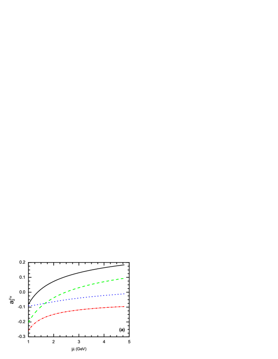
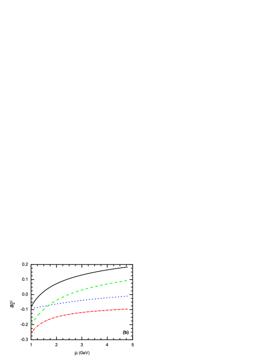
Figure 3: Dependence of $a_{2}$ on the renormalization scale $\mu$ for (a) $B\to J/\Psi K$ and (b) $B\to\eta_{c}K$ decays. The solid ( dashed ) curve stands for $a_{2}$ at NLO (LO) level without the vertex corrections, while the dotted ( dash-dotted ) curve refers to the real (imaginary) part of the $a_{2}$ at NLO level with the vertex corrections.

Since both $B\to J/\Psi K$ and $\eta_{c}K$ are color-suppressed decays, the Wilson coefficient $a_{2}$ in general plays the dominate role. It is instructive to check the variation of $a_{2}$ at LO or NLO level, with or without the inclusion of the NLO vertex corrections. From Figs.3a and 3b, one can see that (a) the $\mu$-dependence of $a_{2}(J/\Psi K)$ and $a_{2}(\eta_{c}K)$ are very similar; (b) the $\mu$-dependence of $a_{2}$ is decreased effectively due to the inclusion of the NLO vertex corrections; and (c) the vertex correction provides a large imaginary part to $a_{2}$, and therefore an effective enhancement of $|a_{2}|$ due to the vertex correction is expected.

III Numerical results and Discussions

III.1 Branching ratios

The input parameters and the wave functions to be used in the numerical calculations are given in Appendix B.

Firstly, we find the pQCD predictions for the corresponding form factors at zero momentum transfer:

$$F^{B\to K}_{0}(q^{2}=0) = 0.32^{+0.05}_{-0.05}(\omega_{b})\;,$$ (29)

for $f_{B}=0.19$ GeV, and $\omega_{b}=0.40\pm 0.04$GeV. It agrees very well with that obtained in QCD sum rule calculationsmelic1 .

Now we calculate the branching ratios for those considered decay modes. With the complete decay amplitudes, we can obtain the decay width for the considered decays,

$$\Gamma(B\to M_{2}K)=\frac{G_{F}^{2}m_{B}^{3}}{32\pi}(1-r^{2})\left|{\cal M}(B\to M_{2}K)\right|^{2},$$ (30)

where $r=m_{J/\Psi}/m_{B}$ or $m_{\eta_{c}}/m_{B}$.

By using the input parameters and wave functions as given in Appendix B, we find the LO and NLO pQCD predictions (in unit of $10^{-4}$) for the CP-averaged branching ratios of the four $B\to J/\Psi K$ and $\eta_{c}K$ decays and show them in the Table 1. The predictions listed in the column one are the LO pQCD predictions by setting $\mu_{0}=1.0$ GeV. The predictions listed in the column two is the NLO pQCD prediction by setting $\mu_{0}=1.0$. The first theoretical error in these entries arises from the B meson wave function shape parameter $\omega_{b}=0.40\pm 0.04$ and the decay constants $f_{J/\Psi}=0.405\pm 0.014$ GeV and/or $f_{\eta_{c}}=0.420\pm 0.050$ GeV. The second error is from the combination of the uncertainties of Gegenbauer moments $a_{1}^{K}=0.17\pm 0.17$ and/or $a_{2}^{K}=0.115\pm 0.115$. In the fourth column of Table 1, as a comparison, we also cite the typical theoretical predictions obtained previously by using various approaches or models ck00 ; cheng01 ; chao2 ; melic .

In the last column of Table 1, we list the world averages of the experimental measurements pdg2008 ; hfag2008 . One can see that the LO pQCD predictions for the branching ratios are indeed much smaller than the measured values, but the pQCD predictions with the inclusion of the vertex corrections can enhance the branching ratios evidently for both $B\to J/\Psi K$ and $B\to\eta_{c}K$ decays. When the NLO enhancement are included, the pQCD predictions are basically consistent with the data within the still large theoretical errors. Of course, the central values are still about 40% smaller than the measured values. There is still some room left for non-perturbative contributions.

Table 1: The LO and NLO pQCD predictions (in unit of $10^{-4}$ ) of $Br(B\to J/\Psi K)$ and $Br(B\to\eta_{c}K)$. For comparison, we also cite the typical theoretical predictions as given in previous literatures (in the fourth column), and the measured values pdg2008 ; hfag2008 .

Channels	LO	NLO	Others	Data
$B^{0}\to J/\Psi K^{0}$	$1.1^{+0.8+0.9}_{-0.5-0.5}$	$5.2^{+1.0+3.4}_{-0.9-2.6}$	$\sim 1.0$ ck00	$8.71\pm 0.32$
$B^{+}\to J/\Psi K^{+}$	$1.2^{+0.9+0.9}_{-0.5-0.5}$	$5.6^{+1.0+3.6}_{-0.9-2.8}$	$\sim 3.3$ melic	$10.07\pm 0.35$
$B^{0}\to\eta_{c}K^{0}$	$0.8^{+0.5+0.1}_{-0.3-0.1}$	$5.5^{+2.1+1.0}_{-1.7-1.0}$	$\sim 2$chao2 ; chen05	$8.9\pm 1.6$
$B^{+}\to\eta_{c}K^{+}$	$0.8^{+0.5+0.2}_{-0.2-0.1}$	$5.9^{+2.2+1.2}_{-1.8-1.1}$	$\sim 2$melic ; chen05	$9.1\pm 1.3$

Now we investigate in more detail why the vertex corrections can provide a significant enhancement. The total decay amplitudes as given in Eqs.(20) and (22) can be in re-written in the following form

$$M = \left[F_{C}+F_{P}\right]_{Fac.}+\left[M_{T}+M_{P}\right]_{Spec.},$$ (31)

where $F_{C}$ and $F_{P}$ stands for the “color-suppressed” and the penguin part of the factorizable contribution, coming from the emission diagram Fig.1a and 1b; while $M_{T}$ and $M_{P}$ stands for the “Tree” and the penguin part of the nonfactorizable contribution, coming from the spectator diagram Fig.1c and 1d. From Eq. (20), for example, it ie easy to separate the total decay amplitude ${\cal M}(B\to J/\Psi K)$ into the following four parts

$$F_{C} = F_{J/\Psi K}^{V-A}f_{J/\Psi}\;V_{cb}^{*}V_{cs}\;a_{2};$$

$$F_{P} = -F_{J/\Psi K}^{V-A}f_{J/\Psi}\;V_{tb}^{*}V_{ts}\;\left(a_{3}+a_{5}+a_{7}+a_{9}\right);$$ (32)

$$M_{T} = M_{J/\Psi K}^{V-A}\;V_{cb}^{*}V_{cs}\;C_{2};$$

$$M_{P} = -M_{J/\Psi K}^{V-A}\;V_{tb}^{*}V_{ts}\;\left(C_{4}-C_{6}-C_{8}+C_{10}\right)$$ (33)

By numerical calculations, we find easily the numerical values (in unit of $10^{-3}$) of the individual parts and the total decay amplitude of ${\cal M}(B\to J/\Psi K)$ at the LO and NLO level:

$${\cal M}^{LO} = \underbrace{-1.147}_{F_{C}}-\underbrace{0.092}_{F_{P}}+\underbrace{(1.487+i0.529)}_{M_{T}}+\underbrace{(0.046+i0.004)}_{M_{P}},$$ (34)

$$= 0.294+i0.533,$$

$${\cal M}^{NLO} = \underbrace{(-0.546-i1.433)}_{F_{C}}+\underbrace{(0.004-i0.038)}_{F_{P}}+\underbrace{(1.367+i0.485)}_{M_{T}}+\underbrace{(0.037+i0.002)}_{M_{P}},$$ (35)

$$= 0.862-i0.984,$$

and the ratio of the square of the decay amplitude ${\cal M}^{NLO}$ and ${\cal M}^{LO}$ is

$$R_{M}(B\to J/\Psi K)=\frac{\left|{\cal M}^{NLO}\right|^{2}}{\left|{\cal M}^{LO}\right|^{2}}=4.62.$$ (36)

For $B\to\eta_{c}K$ decay, we find the similar result: $R_{M}(B\to\eta_{c}K)=7.0$.

From the above numerical results, it is easy to see that

• As generally expected, both the the factorizable penguin contribution ( $F_{P}$) and the nonfactorizable part ( $M_{P}$) to the total decay amplitude are always small in magnitude ( less than $10\%$), when compared with the ”Tree” and ”Color-suppressed” parts ($M_{T}$ and $F_{C}$).

• At the leading order, $F_{C}=-1.147$ is large in size, but largely canceled by the real part of $M_{T}$ ( ${\rm Re}(M_{T})=1.487$ ) when one sums up the factorizable and nonfactorizable contributions. This strong cancelation results in a small LO pQCD prediction for the decay rates.

• At the next-to-leading order, the NLO Wilson coefficients will be used. The penguin part $F_{P}$ and $M_{P}$ remain small in magnitude. The variations of $M_{T}$ and $M_{P}$ due to the replacement of the LO Wilson coefficients by the NLO ones are also small as expected. For the “color-suppressed” $F_{C}$ part, however, things become much different. The real part of $F_{C}$ changes from $-1.147$ to $-0.546$, the previous large cancelation between the real parts of $F_{C}$ and $M_{T}$ become weak significantly, while a large imaginary part ${\rm Im}(F_{C})=-1.433$ is also produced. These two changes lead to a large $|{\cal M}^{NLO}|^{2}$ and consequently a large NLO pQCD prediction of the branching ratios.

• Although the NLO pQCD predictions for the branching ratios of the considered decays are consistent with the date within the still large theoretical uncertainties, but the central values of the NLO pQCD predictions, as listed in Table 1, are still about $60\%$ of the measured values. Certainly, there are still some room left for the non-perturbative long distance effects or other unknown high order corrections.

• Among the three kinds of known NLO contributions in the pQCD approach, only the vertex corrections are relevant to $B\to(J/\Psi,\eta_{c})K$ decays and taken into account here. Other possible NLO contributions coming from the Feynman diagrams as shown in Figs.5-7 in Ref. xiao08 are still unknown at present. But they are generally expected to be the small part of the NLO contributions in the pQCD factorization approachnlo05 ; xiao08 .

• In Ref. plb542 , the authors attempted to estimate the soft rescattering effect for $B^{+}\to J/\Psi K^{+}$ decay and concluded that such effect is comparable in size with the experimental one. But it is worth mentioning that the estimation as presented in Ref. plb542 has a very large theoretical uncertainty. We believe that the long distance effects for the considered decays are exist and may be large, but much more careful studies should be made before one can find an reliable estimation about them cheng01 ; chen05 ; li07a .

As discussed in previous section, we choose $\mu_{0}=1.0$ GeV as the lower cut-off of the hard scale $t$. It should be noted that in the considered decay channels, the characteristic hard energy scale maybe smaller than 1 GeV, while all the meson distribution amplitudes are defined at 1 GeV. In the numerical integration, we therefore should set the Wilson coefficients $C_{i}(t)=C_{i}(1\;$GeV$)$ whenever $t\leq 1$ GeV to ensure the reliability of our perturbative calculations.

Now we turn to study the ratios of the branching ratios for some phenomenologically relevant decay modes. One advantage of the ratios is the possible cancelation of the theoretical uncertainties of individual calculations. Using the data of the measured branching ratios as given in Ref. pdg2008 , the three ratios $R_{i}^{exp}$ can be defined as the following

$$R_{1}^{exp} = \frac{Br(B^{+}\to\eta_{c}K^{+})}{Br(B^{+}\to J/\Psi K^{+})}=0.90\pm 0.13,$$

$$R_{2}^{exp} = \frac{Br(B^{0}\to\eta_{c}K^{0})}{Br(B^{0}\to J/\Psi K^{0})}=1.02\pm 0.19,$$

$$R_{3}^{exp} = \frac{Br(B^{0}\to\eta_{c}K^{0})}{Br(B^{-}\to\eta_{c}K^{-})}=0.88\pm 0.16\;.$$ (37)

Table 2: The ratios $R_{i}$ of the pQCD predictions for the branching ratios. The ratios as given in PDG 2008 pdg2008 are also shown in the last column.

Ratios	LO	NLO	Data
$R_{1}$	$0.7^{+0.9}_{-0.4}$	$1.05^{+1.14}_{-0.42}$	$0.90\pm 0.13$
$R_{2}$	$0.7^{+1.3}_{-0.3}$	$1.06^{+1.23}_{-0.43}$	$1.02\pm 0.19$
$R_{3}$	$1.0^{+0.6}_{-0.4}$	$0.93^{+0.52}_{-0.27}$	$0.88\pm 0.16$

By comparing the pQCD predictions of the ratios and the measured ones, as listed in Table 2, we can see that (a) the consistency between the pQCD prediction for the ratios and the measured ones is improved significantly when the NLO contributions are taken into account; (b) the theoretical uncertainties are still large because of our poor knowledge about the Gegenbauer moments $a_{1,2}^{K}$.

In short, from the above pQCD predictions for the branching ratios and the detailed phenomenological analysis, we can conclude that the pQCD predictions for the branching ratios become close to the data due to the significant enhancement of the NLO vertex corrections.

III.2 CP-violating asymmetries

Now we turn to the evaluations of the CP-violating asymmetries of $B\to M_{2}\;M_{3}$ decays in pQCD approach. For the charged B meson decays,the direct CP-violating asymmetries ${\cal A}_{CP}^{dir}$ can be defined as usual. For both $B^{+}\to J/\Psi K^{+}$ and $\eta_{c}K^{+}$ decays, there are no direct CP violation, since there is no weak phase appeared in their decay amplitude, as can be seen easily in Eqs. (20) and (22). This theoretical expectation agrees well with the data pdg2008 ; hfag2008 :

$${\cal A}_{CP}^{dir}(B^{+}\to J/\Psi K^{+}) = 0.017\pm 0.016\;,$$

$${\cal A}_{CP}^{dir}(B^{+}\to\eta_{c}K^{+}) = -0.16\pm 0.08\;.$$ (38)

which are consistent with zero within $2\sigma$ errors.

For the $B^{0}\to M_{2}M_{3}$ decays, because these decays are neutral B meson decays, so we should consider the effects of $B^{0}-\bar{B}^{0}$ mixing. The direct and mixing induced CP-violating asymmetries ${\cal A}_{CP}^{dir}$ and ${\cal A}_{CP}^{mix}$ can be written as

$${\cal A}_{CP}^{dir}=\frac{\left|\lambda_{CP}\right|^{2}-1}{1+|\lambda_{CP}|^{2}},\quad{\cal A}_{CP}^{mix}=\frac{2Im(\lambda_{CP})}{1+|\lambda_{CP}|^{2}},$$ (39)

where the CP-violating parameter $\lambda_{CP}$ is

$$\lambda_{CP}=\eta_{f}\frac{V_{tb}^{*}V_{td}\langle f|H_{eff}|\overline{B}^{0}\rangle}{V_{tb}V_{td}^{*}\langle f|H_{eff}|B^{0}\rangle}=\eta_{f}e^{-2i\beta}\frac{\langle f|H_{eff}|\overline{B}^{0}\rangle}{\langle f|H_{eff}|B^{0}\rangle},$$ (40)

where $\eta_{f}$ is the CP-eigenvalue of the final states. By using the the input parameters as given in Appendix B, we find the following pQCD predictions

$${\cal A}_{CP}^{dir}(B^{0}\to J/\Psi K_{S}^{0}) = {\cal A}_{CP}^{dir}(B^{0}\to\eta_{c}K_{S}^{0})\approx 0\;,$$

$${\cal A}_{CP}^{mix}(B^{0}\to J/\Psi K_{S}^{0}) = {\cal A}_{CP}^{mix}(B^{0}\to\eta_{c}K_{S}^{0})=\left(70.9^{+2.8}_{-2.7}\right)\%,$$ (41)

where the dominant error comes from $\bar{\rho}=0.135^{+0.031}_{-0.016}$ and $\bar{\eta}=0.349^{+0.015}_{-0.017}$ pdg2008 . It is easy to see that the pQCD predictions for CP -violating asymmetries agree perfectly with the experimental measurements pdg2008 ; hfag2008 .

IV Summary

In this paper, we calculated the branching ratios and CP-violating asymmetries of the four $B\to(J/\Psi,\eta_{c})K$ decays by employing the pQCD factorization approach with the inclusion of currently known NLO contributions.

From our numerical calculations and phenomenological analysis, we found the following results:

• The inclusion of the known NLO contributions can result in a factor of five enhancements to the leading order results. The NLO pQCD predictions for the branching ratios are the following

  $$Br(B^{0}\to J/\Psi K^{0}) = 5.2^{+3.5}_{-2.8}\times 10^{-4},$$

  $$Br(B^{+}\to J/\Psi K^{+}) = 5.6^{+3.7}_{-2.9}\times 10^{-4},$$

  $$Br(B^{0}\to\eta_{c}K^{0}) = 5.5^{+2.3}_{-2.0}\times 10^{-4},$$

  $$Br(B^{+}\to\eta_{c}K^{+}) = 5.9^{+2.5}_{-2.1}\times 10^{-4}.$$ (42)

  Although the central values of the pQCD predictions are still $40\%$ smaller than the measured ones, they basically agree with the data within $2\sigma$ errors. One can also see that, on the other hand, there are still some room left for the non-perturbative contributions.

• The pQCD predictions for the CP-violating asymmetries of the considered decays also agree perfectly with the data.

• In this paper, only those currently known NLO contributions have been taken into account. To obtain a complete NLO calculations in the pQCD approach, the still missing pieces should be evaluated as soon as possible.

Appendix A Related Functions

We show here the hard function $h_{i}$’s, coming from the Fourier transformations of the function $H^{(0)}$,

$$h_{e}(x_{1},x_{3},b_{1},b_{3}) = K_{0}\left(\sqrt{x_{1}x_{3}(1-r^{2})}m_{B}b_{1}\right)\left[\theta(b_{1}-b_{3})K_{0}\left(\sqrt{x_{3}(1-r^{2})}m_{B}b_{1}\right)\right.$$ (43)

$$\;\left.\cdot I_{0}\left(\sqrt{x_{3}(1-r^{2})}m_{B}b_{3}\right)+\theta(b_{3}-b_{1})K_{0}\left(\sqrt{x_{3}(1-r^{2})}m_{B}b_{3}\right)\right.$$

$$\;\left.\cdot I_{0}\left(\sqrt{x_{3}(1-r^{2})}m_{B}b_{1}\right)\right]S_{t}(x_{3}),$$

$$h_{f}(x_{1},x_{2},x_{3},b_{1},b_{2}) = \biggl{\{}\theta(b_{2}-b_{1})\mathrm{I}_{0}(m_{B}\sqrt{x_{1}x_{3}(1-r^{2})}b_{1})\mathrm{K}_{0}(m_{B}\sqrt{x_{1}x_{3}(1-r^{2})}b_{2})$$ (44)

$$+ (b_{1}\leftrightarrow b_{2})\biggr{\}}\cdot\left(\begin{matrix}\mathrm{K}_{0}(m_{B}F_{(1)}b_{2}),&\text{for}\quad F^{2}_{(1)}>0\\ \frac{\pi i}{2}\mathrm{H}_{0}^{(1)}(m_{B}\sqrt{|F^{2}_{(1)}|}\ b_{2}),&\text{for}\quad F^{2}_{(1)}<0\end{matrix}\right),$$

where $J_{0}$ is the Bessel function, $K_{0}$ and $I_{0}$ are the modified Bessel functions with $K_{0}(-ix)=-(\pi/2)Y_{0}(x)+i(\pi/2)J_{0}(x)$, and $F_{(1)}^{2}$ is defined by

$$F^{2}_{(1)} = (x_{1}-x_{2})(x_{3}+(x_{2}-x_{3})r^{2})+r_{c}^{2}\;.$$ (45)

The threshold resummation form factor $S_{t}(x_{i})$ can be found in Ref. tls .

The Sudakov factors used in the text are defined as

$$S_{ab}(t) = s\left(x_{1}m_{B}/\sqrt{2},b_{1}\right)+s\left(x_{3}m_{B}/\sqrt{2},b_{3}\right)+s\left((1-x_{3})m_{B}/\sqrt{2},b_{3}\right)$$ (46)

$$-\frac{1}{\beta_{1}}\left[\ln\frac{\ln(t/\Lambda)}{-\ln(b_{1}\Lambda)}+\ln\frac{\ln(t/\Lambda)}{-\ln(b_{3}\Lambda)}\right],$$

$$S_{cd}(t) = s\left(x_{1}m_{B}/\sqrt{2},b_{1}\right)+s\left(x_{2}m_{B}/\sqrt{2},b_{2}\right)+s\left((1-x_{2})m_{B}/\sqrt{2},b_{2}\right)$$ (47)

$$+s\left(x_{3}m_{B}/\sqrt{2},b_{1}\right)+s\left((1-x_{3})m_{B}/\sqrt{2},b_{1}\right)$$

$$-\frac{1}{\beta_{1}}\left[2\ln\frac{\ln(t/\Lambda)}{-\ln(b_{1}\Lambda)}+\ln\frac{\ln(t/\Lambda)}{-\ln(b_{2}\Lambda)}\right],$$

where the function $s(q,b)$ are defined in the Appendix A of Ref. luy01 . The scale $t_{i}$’s in the above equations are chosen as

$$t_{e}^{1} = {\rm max}(\sqrt{x_{3}(1-r^{2})}m_{B},1/b_{1},1/b_{3}),$$

$$t_{e}^{2} = {\rm max}(\sqrt{x_{1}(1-r^{2})}m_{B},1/b_{1},1/b_{3}),$$

$$t_{f} = {\rm max}(\sqrt{x_{1}x_{3}(1-r^{2})}m_{B},\sqrt{(x_{1}-x_{2})x_{3}(1-r^{2})+r_{c}^{2}}m_{B},1/b_{1},1/b_{2}),$$ (48)

where $r=m_{M_{2}}/m_{B}(M_{2}=J/\Psi,\eta_{c})$,$r_{c}=m_{c}/m_{B}$. The scale $t_{i}$’s are chosen as the maximum energy scale appearing in each diagram in order to kill the large logarithmic radiative corrections.

Appendix B Input parameters and wave functions

The masses, decay constants, QCD scale and $B$ meson lifetime are the following

$$f_{J/\Psi} = 0.405{\rm GeV},\quad f_{K}=0.16{\rm GeV},\quad f_{\eta_{c}}=0.42{\rm GeV},\quad m_{W}=80.41{\rm GeV},$$

$$m_{\eta_{c}} = 2.98{\rm GeV},\quad m_{B}=5.2794{\rm GeV},\quad m_{J/\Psi}=3.097{\rm GeV},$$

$$\tau_{B^{+}} = 1.643{\rm ps},\quad\tau_{B^{0}}=1.53{\rm ps}.$$ (49)

For the CKM matrix elements, here we adopt the Wolfenstein parametrization for the CKM matrix, and take $\lambda=0.2257,A=0.814,\bar{\rho}=0.135$ and $\bar{\eta}=0.349$ pdg2008 .

As for $B$ meson wave function, we make use of the same parameterizations as in Ref. luy01 . We adopt the model

$$\phi_{B}(x,b) = N_{B}x^{2}(1-x)^{2}\mathrm{exp}\left[-\frac{m_{B}^{2}\ x^{2}}{2\omega_{b}^{2}}-\frac{1}{2}(\omega_{b}b)^{2}\right],$$ (50)

where $\omega_{b}$ is a free parameter and we take $\omega_{b}=0.40\pm 0.04$ GeV in numerical calculations, and $N_{B}=91.745$ is the normalization factor for $\omega_{b}=0.40$.

For the vector $J/\Psi$ meson, we take the wave function as follows,

$$\Phi_{J/\Psi}(x) = \frac{1}{\sqrt{2N_{c}}}\bigg{\{}m_{J/\Psi}\epsilon/\,_{L}\phi_{J/\Psi}^{L}(x)+\epsilon/\,_{L}P/\phi_{J/\Psi}^{t}(x)\bigg{\}}\;.$$ (51)

Here, $\phi^{L}$ denote for the twist-2 DA’s, and $\phi^{t}$ for the twist-3 ones, both of them have experimental and theoretical basisbc04 . $x$ represents the momentum fraction of the charm quark inside the charmonium. The $J/\Psi$ meson asymptotic distribution amplitudes read as bc04

$$\phi_{J/\Psi}^{L}(x) = 9.58\frac{f_{J/\Psi}}{2\sqrt{2N_{c}}}x(1-x)\left[\frac{x(1-x)}{1-2.8x(1-x)}\right]^{0.7}\;,$$

$$\phi_{J/\Psi}^{t}(x) = 10.94\frac{f_{J/\Psi}}{2\sqrt{2N_{c}}}(1-2x)^{2}\left[\frac{x(1-x)}{1-2.8x(1-x)}\right]^{0.7}\;.$$ (52)

It is easy to see that both the twist-2 and twist-3 DA’s vanish at the end points due to the factor $[x(1-x)]^{0.7}$.

For pseudoscalar meson $\eta_{c}$, the wave function is the form of

$$\Phi_{\eta_{c}}(x) = \frac{i}{\sqrt{2N_{c}}}\gamma_{5}\bigg{\{}P/\phi_{\eta_{c}}^{v}+m_{\eta_{c}}\phi_{\eta_{c}}^{s}\bigg{\}}\;.$$ (53)

The twist-2 and twist-3 asymptotic distribution amplitudes, $\phi^{v}$ and $\phi^{s}$, can be written asbc04 ,

$$\phi_{\eta_{c}}^{v}(x) = 9.58\frac{f_{\eta_{c}}}{2\sqrt{2N_{c}}}x(1-x)\left[\frac{x(1-x)}{1-2.8x(1-x)}\right]^{0.7}\;,$$

$$\phi_{\eta_{c}}^{s}(x) = 1.97\frac{f_{\eta_{c}}}{2\sqrt{2N_{c}}}\left[\frac{x(1-x)}{1-2.8x(1-x)}\right]^{0.7}\;.$$ (54)

The twist-2 kaon distribution amplitude $\phi^{A}_{K}$, and the twist-3 ones $\phi_{K}^{P}$ and $\phi_{K}^{T}$ have been parameterized as pball06

$$\phi_{K}^{A}(x) = \frac{f_{K}}{2\sqrt{2N_{c}}}\,6x(1-x)\left[1+a_{1}^{K}C_{1}^{3/2}(t)+a_{2}^{K}C_{2}^{3/2}(t)\right.$$ (55)

$$\hskip 99.58464pt\left.+a_{4}^{K}C_{4}^{3/2}(t)\right],$$

$$\phi^{P}_{K}(x) = \frac{f_{K}}{2\sqrt{2N_{c}}}\,\bigg{[}1+\left(30\eta_{3}-\frac{5}{2}\rho_{K}^{2}\right)C_{2}^{1/2}(t)$$ (56)

$$\hskip 71.13188pt-\,3\left\{\eta_{3}\omega_{3}+\frac{9}{20}\rho_{K}^{2}(1+6a_{2}^{K})\right\}C_{4}^{1/2}(t)\bigg{]}\;,$$

$$\phi^{T}_{K}(x) = \frac{f_{K}}{2\sqrt{2N_{c}}}\,(1-2x)\bigg{[}1+6\left(5\eta_{3}-\frac{1}{2}\eta_{3}\omega_{3}-\frac{7}{20}\rho_{K}^{2}-\frac{3}{5}\rho_{K}^{2}a_{2}^{K}\right)$$ (57)

$$\hskip 99.58464pt\times(1-10x+10x^{2})\bigg{]}\;,\ \ \ \$$

with $t=2x-1$, the Gegenbauer moments $a_{1}^{K}=0.17$, $a^{K}_{2}=0.115$, and $a_{4}^{K}=-0.015$, the parameters $\eta_{3}=0.015$, $\omega_{3}=-3.0$, the mass ratio $\rho_{K}=(m_{u(d)}+m_{s})/m_{K}=m_{K}/m_{0K}$ and the Gegenbauer polynomials $C_{n}^{\nu}(t)$,

$$C_{1}^{3/2}(t) = 3t,\quad C_{2}^{1/2}(t)=\frac{1}{2}\left(3t^{2}-1\right),\quad C_{2}^{3/2}(t)=\frac{3}{2}\left(5t^{2}-1\right),$$

$$C_{4}^{1/2}(t) = \frac{1}{8}\left(3-30t^{2}+35t^{4}\right),\quad C_{4}^{3/2}(t)=\frac{15}{8}\left(1-14t^{2}+21t^{4}\right).$$ (58)

References

- (1) C. Amsler et al. ( Particle Data Group), Phys. Lett. B 667, 1 (2008).
- (2) Heavy Flavor Averaging Group, E. Barberio et al., hep-ex/0808.1297v1; and online update at http://www.slac.stanford.edu/xorg/hfag.
- (3) M. Gourdin,Y.Y. Keum, and X.Y. Pham, Phys. Rev. D 51, 3510 (1995).
- (4) H.Y. Cheng and K.C. Yang, Phys. Rev. D 59, 092004 (1999).
- (5) J. Chay and C. Kim, hep-ph/0009244.
- (6) H.Y. Cheng and K.C. Yang, Phys. Rev. D 63, 074011 (2001).
- (7) H. Boos, J. Reuter and T. Mannel, Phys. Rev. D 70, 036006 (2004); M. Ciuchini, M. Pierini and L. Silvestrini, Phys. Rev. Lett. 95, 221804 (2005).
- (8) Z.Z. Song, C. Meng, Y.J. Gao, and K.T. Chao, Phys. Rev. D 69(2004)054009; Zhong-zhi Song and Kuang-ta Chao , Phys. Lett. B 568(2003)127-134.
- (9) Z. Song,C. Meng, and K.T. Chao, Eur.Phys.J. C 36(2004)365; Ce Meng,Ying-jia Gao, and Kuang-ta Chao, Commun.Theor.Phys. 48, 885(2007);
- (10) B. Melić, Phys. Rev. D 68, 034004 (2003); Phys. Lett. B 591, 91 (2004); L. Li,Z.G. Wang, and T. Huang, Phys. Rev. D 70, 074006 (2004).
- (11) C.-H. V. Chang and H.N. Li, Phys. Rev. D 55, 5577 (1997); T.-W. Yeh and H.N. Li, Phys. Rev. D 56, 1615 (1997).
- (12) C.H. Chen and H.N. Li, Phys. Rev. D 71, 114008 (2005).
- (13) H.N. Li and S. Mishima, J. High Energy Phys. 03, 009 (2007).
- (14) M. Beneke, G. Buchalla, M. Neubert, and C.T. Sachrajda, Phys. Rev. Lett. 83, 1914 (1999);
- (15) H.N. Li, S. Mishima, A.I. Sanda, Phys. Rev. D 72, 114005 (2005).
- (16) Y.Y. Keum, H.N. Li, and A.I. Sanda, Phys. Rev. D 63, 054008 (2001); C.D. Lü, K. Ukai and M.Z. Yang, Phys. Rev. D 63, 074009 (2001); C.H. Chen, Y.Y. Keum, and H.N. Li, Phys. Rev. D 64, 112002 (2001); Y.Y. Keum and H.N. Li, Phys. Rev. D 63, 074006 (2001).
- (17) H.N. Li, Prog.Part. Nucl.Phys. 51, 85 (2003), and reference therein.
- (18) X. Liu, H.S. Wang, Z.J. Xiao, L.B. Guo and C.D. Lü, Phys. Rev. D 73, 074002 (2006); H.S. Wang, X. Liu, Z.J. Xiao, L.B. Guo and C.D. Lü, Nucl. Phys. B 738, 243 (2006); Z.J. Xiao, X.F. Chen and D.Q. Guo, Eur.Phys.J. C 50, 363 (2007); Z.J. Xiao, D.Q Guo and X.F. Chen, Phys. Rev. D 75, 014018 (2007); Z.J. Xiao, X. Liu and H.S. Wang, Phys. Rev. D 75, 034017 (2007).
- (19) A. Ali, G. Kramer, Y. Li, C.D. Lü, Y.L. Shen, W. Wang, and Y.M. Wang, Phys. Rev. D 76, 074018 (2007).
- (20) Z.J. Xiao, Z.Q. Zhang, X. Liu and L.B. Guo, Phys. Rev. D 78, 114001 (2008).
- (21) Z.Q. Zhang and Z.J. Xiao, Eur.Phys.J. C 59, 49 (2009); Z.Q. Zhang and Z.J. Xiao, Commun.Theor.Phys. 51, 885 (2009); J. Liu, R. Zhou and Z.J. Xiao, arXiv:0812.2132[hep-ph].
- (22) Y. Li and C.D. Lü, J. Phys. G 29, 2115 (2003); High Energy Nucl.Phys. 27, 1061 (2003); Y. Li, C.D. Lü, and Z.J. Xiao, J. Phys. G 31, 273 (2005); Y. Li, C.D. Lü, and C.F. Qiao, Phys. Rev. D 73, 094006 (2006).
- (23) Z.J. Xiao, X. Liu, Int.J.Mod.Phys. A 23, 3246 (2008);
- (24) H.N. Li, Phys. Rev. D 66, 094010 (2002).
- (25) H.N. Li and B. Tseng, Phys. Rev. D 57, 443 (1998).
- (26) G. Buchalla, A.J. Buras, and M.E. Lautenbacher, Rev. Mod. Phys. 68, 1125 (1996).
- (27) C.-D. Lü, K. Ukai and M.Z. Yang, Phys. Rev. D 63, 074009 (2001).
- (28) G. Duplanc̆ić and B. Melić, Phys. Rev. D 78(2008)054015.
- (29) P. Colangelo, F. De Fazio and T.N. Pham, Phys. Lett. B 542(2002)71.
- (30) T. Kurimoto, H.N. Li, and A.I. Sanda, Phys. Rev. D 65, 014007 (2001); Phys. Rev. D 67, 054028 (2003).
- (31) A.E. Bondar and V.L. Chernyak, Phys. Lett. B 612, 215(2005).
- (32) P. Ball, J. High Energy Phys. 9809, 005 (1998); P. Ball, J. High Energy Phys. 9901, 010 (1999); P. Ball and R. Zwicky, Phys. Rev. D 71, 014015 (2005); P. Ball, V.M. Braun, and A. Lenz, J. High Energy Phys. 0605, 004 (2006).