Hydrokinetic simulations of nanoscopic precursor films in rough channels

Abstract

We report on simulations of capillary filling of high-wetting fluids in nano-channels with and without obstacles. We use atomistic (molecular dynamics) and hydrokinetic (lattice-Boltzmann) approaches which point out clear evidence of the formation of thin precursor films, moving ahead of the main capillary front. The dynamics of the precursor films is found to obey a square-root law as the main capillary front, $z^{2}(t)\propto t$, although with a larger prefactor, which we find to take the same value for the different geometries (2D-3D) under inspection. The two methods show a quantitative agreement which indicates that the formation and propagation of thin precursors can be handled at a mesoscopic/hydrokinetic level. This can be considered as a validation of the Lattice-Boltzmann (LB) method and opens the possibility of using hydrokinetic methods to explore space-time scales and complex geometries of direct experimental relevance. Then, LB approach is used to study the fluid behaviour in a nano-channel when the precursor film encounters a square obstacle. A complete parametric analysis is performed which suggests that thin-film precursors may have an important influence on the efficiency of nanochannel-coating strategies.

1 Introduction

Micro- and nano-hydrodynamic flows are prominent in many applications in material science, chemistry and biology [1, 2, 3, 4, 5, 6, 7, 8, 9, 12, 10, 11]. A thorough fundamental understanding as well as the development of corresponding efficient computational tools are demanded. The formation of thin precursor films in capillary experiments with highly wetting fluids (near-zero contact angle) has been reported by a number of experiments and theoretical works [13, 14, 15, 16, 17], mostly in connection with droplet spreading, and only very recently [18] for the case of capillary filling. In this latter case the presence of precursor films could help to reduce the drag, and this could have an enormous economic impact as mechanical technology is miniaturized, microfluidic devices become more widely used, and biomedical analysis moves aggressively towards lab on a chip technologies. In this direction, patterned channels [19] and more specifically ultra-hydrophobic surfaces have been considered [20, 21]. At microscopic scales, inertia subsides and fluid motion is mainly governed by the competition between dissipation, surface-tension and external pressure. In this realm, the continuum assumption behind the macroscopic description of fluid flow goes often under question, typical cases in point being slip-flow at solid walls and moving a contact line of liquid/gas interface on solid walls [1, 13]. In order to keep a continuum description at nanoscopic scales and close to the boundaries, the hydrodynamic equations are usually enriched with generalised boundary conditions, designed in such a way as to collect the complex physics of fluid-wall interactions into a few effective parameters, such as the slip length and the contact angle [22, 23]. A more radical approach is to quit the continuum level and turn directly to the atomistic description of fluid flows as a collection of moving molecules [24], typically interacting via a classical 6-12 Lennard-Jones potential. This approach is computationally demanding, thus preventing the attainment of space and time macroscopic scales of experimental interest. In between the macroscopic and microscopic vision, a mesoscopic approach has been lately developed in the form of minimal lattice versions of the Boltzmann kinetic equation [25, 26]. This mesoscopic/hydro-kinetic approach offers a compromise between the two methods, i.e. physical realism combined with high computational efficiency. By definition, such a mesoscopic approach is best suited to situations where molecular details, while sufficiently important to require substantial amendments of the continuum assumption, still possess a sufficient degree of universality to allow general continuum symmetries to survive, a situation that we shall dub supra-molecular for simplicity. Lacking a rigorous bottom-up derivation, the validity of the hydro-kinetic approach for supra-molecular physics must be assessed case-by-case, a program which is already counting a number of recent successes [27, 28, 29, 30]. The aim of this paper is two-fold. First, we validate the Lattice-Boltzmann (LB) hydro-kinetic method in another potentially ’supramolecular’ situation, i.e. the formation and propagation of precursor films in capillary filling at nanoscopic scales. We employ both MD and hydrokinetic simulations, finding quantitative agreement for both bulk quantities and local density profiles, at all times during the capillary filling process. Then, we carry out a complete LB study of a nanochannel in the presence of a square obstacle for a large range of value for the different parameters at play. These results seem to suggest that, by forming and propagating ahead of the main capillary front, thin-film precursors may manage to hide the chemical/geometrical details of the nanochannel walls, thereby exerting a major influence on the efficiency of nanochannel-coating strategies [31, 32]. The paper is organised as follows: in the first two sections the models employed are presented with some details. In section IV, the numerical results are discussed: first the study of a nanochannel for a complete wetting is presented and, then, the LB analysis of a nanochannel in presence of a square obstacle is reported. Finally, conclusions are made.

2 Lattice-Boltzmann model

In this work we use the multicomponent LB model proposed by Shan and Chen [33]. This model allows for distribution functions of an arbitrary number of components, with different molecular mass:

$$f^{k}_{i}({\bm{x}}+{\bm{c}}_{i}\Delta t,t+\Delta t)-f^{k}_{i}({\bm{x}},t)=-\frac{\Delta t}{\tau_{k}}\left[f^{k}_{i}({\bm{x}},t)-f_{i}^{k(eq)}({\bm{x}},t)\right]$$ (1)

where $f^{k}_{i}(\bm{x},t)$ is the kinetic probability density function associated with a mesoscopic velocity $\bm{c}_{i}$ for the $k$th fluid, $\tau_{k}$ is a mean collision time of the $k$th component (with $\Delta t$ a time step), and $f^{k(eq)}_{i}({\bm{x}},t)$ the corresponding equilibrium function. The collision-time is related to kinematic viscosity by the formula $\nu_{k}=\frac{1}{3}(\tau_{k}-\frac{1}{2})$. For a two-dimensional 9-speed LB model (D2Q9) $f^{k(eq)}_{i}({\bm{x}},t)$ takes the following form [26]:

$$f^{k(eq)}_{0} = \alpha_{k}n_{k}-\frac{2}{3}n_{k}{\bf u}_{k}^{eq}\cdot{\bf u}_{k}^{eq}$$ (2)

$$f^{k(eq)}_{i} = \frac{(1-\alpha_{k})n_{k}}{5}+\frac{1}{3}n_{k}{\bf c}_{i}\cdot{\bf u}_{k}^{eq}$$

$$+ \frac{1}{2}n_{k}({\bf c}_{i}\cdot{\bf u}_{k}^{eq})^{2}-\frac{1}{6}n_{k}{\bf u}_{k}^{eq}\cdot{\bf u}_{k}^{eq}\;\;\;\textrm{for i=1$\ldots$4}$$

$$f^{k(eq)}_{i} = \frac{(1-\alpha_{k})n_{k}}{20}+\frac{1}{12}n_{k}{\bf c}_{i}\cdot{\bf u}_{k}^{eq}$$

$$+ \frac{1}{8}n_{k}({\bf c}_{i}\cdot{\bf u}_{k}^{eq})^{2}-\frac{1}{24}n_{k}{\bf u}_{k}^{eq}\cdot{\bf u}_{k}^{eq}\;\;\;\textrm{for i=5$\ldots$8}$$

In the above equations ${\bf c}_{i}$’s are discrete velocities, defined as follows

$${\bf c}_{i}=\left\{\begin{array}[]{l}0,i=0,\\ \left(cos\frac{(i-1)\pi}{2},sin\frac{(i-1)\pi}{2}\right),i=1-4\\ \sqrt{2}\left(cos[\frac{(i-5)\pi}{2}+\frac{\pi}{4}],sin[\frac{(i-5)\pi}{2}+\frac{\pi}{4}]\right),i=5-8\end{array}\right.$$ (5)

where $\alpha_{k}$ is a free parameter related to the sound speed of the $k$th component, according to $(c_{s}^{k})^{2}=\frac{3}{5}(1-\alpha_{k})$; $n_{k}=\sum_{i}f^{k}_{i}$ is the number density of the $k$th component. The mass density is defined as $\rho_{k}=m_{k}n_{k}$, and the fluid velocity of the $k$th fluid ${\bf u}_{k}$ is defined through $\rho_{k}{\bf u}_{k}=m_{k}\sum_{i}{\bf c}_{i}f_{i}^{k}$, where $m_{k}$ is the molecular mass of the $k$th component. The equilibrium velocity ${\bf u}_{k}^{eq}$ is determined by the relation

$$\rho_{k}{\bf u}_{k}^{eq}=\rho_{k}{\bf U}+\tau_{k}{\bf F}_{k}$$ (6)

where ${\bf U}$ is the common velocity of the two components. To conserve momentum at each collision in the absence of interaction (i.e. in the case of ${\bf F}_{k}=0$) ${\bf U}$ has to satisfy the relation

$${\bf U}=\left(\sum_{i}^{s}\frac{\rho_{k}{\bf u}_{k}}{\tau_{k}}\right)/\left(\sum_{i}^{s}\frac{\rho_{k}}{\tau_{k}}\right)\;.$$ (7)

The interaction force between particles is the sum of a bulk and a wall components. The bulk force is given by

$${\bf F}_{1k}({\bf x})=-\Psi_{k}({\bm{x}})\sum_{{\bm{x}}^{\prime}}\sum_{\bar{k}=1}^{s}G_{k\bar{k}}\Psi_{\bar{k}}({\bm{x}}^{\prime})({\bm{x}}^{\prime}-{\bm{x}})$$ (8)

where $G_{k\bar{k}}$ is symmetric and $\Psi_{k}$ is a function of $n_{k}$. In our model, the interaction-matrix is given by

$$G_{k\bar{k}}=\left\{\begin{array}[]{l}g_{k\bar{k}},|{\bm{x}}^{\prime}-{\bm{x}}|=1,\\ g_{k\bar{k}}/4,|{\bm{x}}^{\prime}-{\bm{x}}|=\sqrt{2},\\ 0,\textrm{otherwise}.\end{array}\right.$$ (9)

where $g_{k\bar{k}}$ is the strength of the inter-particle potential between components $k$ and $\bar{k}$. In this study, the effective number density $\Psi_{k}(n_{k})$ is taken simply as $\Psi_{k}(n_{k})=n_{k}$. Other choices would lead to a different equation of state (see below).

At the fluid/solid interface, the wall is regarded as a phase with constant number density. The interaction force between the fluid and wall is described as

$${\bf F}_{2k}({\bf x})=-n_{k}({\bm{x}})\sum_{{\bm{x}}^{\prime}}g_{kw}\rho_{w}({\bm{x}}^{\prime})({\bm{x}}^{\prime}-{\bm{x}})$$ (10)

where $\rho_{w}$ is the number density of the wall and $g_{kw}$ is the interaction strength between component $k$ and the wall. By adjusting $g_{kw}$ and $\rho_{w}$ , different wettabilities can be obtained. This approach allows the definition of a static contact angle $\theta$, by introducing a suitable value for the wall density $\rho_{w}$ [34], which can span the range $\theta\in[0^{o}:180^{o}]$. In that work [34], for the first time to the best of our knowledge, this phenomenological definition of the contact angle was put forward and the multi-component lattice Boltzmann method was used to study the displacement of a two-dimensional immiscible droplet subject to gravitational forces in a channel. In particular, the dynamic behavior of the droplet was analysed, and the effects of the contact angle, Bond number (the ratio of gravitational to surface forces), droplet size, and density and viscosity ratios of the droplet to the displacing fluid were investigated. It is worth noting that, with this method, it is not possible to know “a priori” the value of the contact angle from the phenomenological parameters. Thus, an “a posteriori” map of the value of the static contact angle versus the value of the interaction strength $g_{w}$ has to be obtained. To this aim, we have carried out several simulations of a static droplet attached to a wall for different values of $g_{w}$ [34, 35]. In particular, in our work, the value of the static contact angle has been computed directly as the slope of the contours of near-wall density field, and independently through the Laplace’s law, $\Delta P=\frac{2\gamma cos\theta}{H}$, where $H$ is the channel height. The value so obtained is computed within an error $\sim 2\%-3\%$. Recently, a different approach has been proposed, which is able to give an “a priori” estimate of the static contact angle from the phenomenological parameter [36]. Nevertheless, we have preferred to retain our “a posteriori” method for its simplicity and efficiency.

In a region of pure $k$th component, the pressure is given by $p_{k}=(c_{s}^{k})^{2}m_{k}n_{k}$, where $(c_{s}^{k})^{2}=\frac{3}{5}(1-\alpha_{k})$. To simulate a multiple component fluid with different densities, we let $(c_{s}^{k})^{2}m_{k}=c_{0}^{2}$, where $c_{0}^{2}=1/3$. Then, the pressure of the whole fluid is given by $p=c_{0}^{2}\sum_{k}n_{k}+\frac{3}{2}\sum_{k,\bar{k}}g_{k,\bar{k}}\Psi_{k}\Psi_{\bar{k}}$, which represents a non-ideal gas law.

The Chapman-Enskog expansion [26] shows that the fluid mixture follows the Navier-Stokes equations for a single fluid:

$$\partial_{t}\rho+\nabla\cdot(\rho{\bf u}) = 0,$$ (11)

$$\rho[\partial_{t}{\bm{u}}+({\bm{u}}\cdot{\bm{\nabla}}){\bm{u}}] = -{\bf\nabla}{P}+{\bm{F}}+{\bm{\nabla}}\cdot(\mu({\bm{\nabla}}{\bm{u}}+{\bm{u}}{\bm{\nabla}}))$$

where $\rho=\sum_{k}\rho_{k}$ is the total density of the fluid mixture, the whole fluid velocity ${\bf u}$ is defined by $\rho{\bf u}=\sum_{k}\rho_{k}{\bf u}_{k}+\frac{1}{2}\sum_{k}{\bf F}_{k}$ and the dynamic viscosity is given by $\mu=\rho\nu=\sum_{k}\mu_{k}=\sum_{k}(\rho_{k}\nu_{k})$.

To the purpose of analysing the physics of film precursors, it is important to notice that , in the limit where the hard-core repulsion is negligible, both the Shan-Chen pseudo-potential and Van der Waals interactions predict a non-ideal equation of state, in which the leading correction to the ideal pressure is $\propto\rho^{2}$. Therefore, both models obey the Maxwell area rule  [35].

3 MD model

In the Molecular Dynamics simulation we use the simplest model, consisting of a fluid of point-size particles that interact via a Lennard-Jones potential. Henceforth all lengths will be quoted in units of $\sigma$, the atom diameter. The snapshot in Fig. 1b, illustrates our simulation geometry. We consider a cylindrical nanotube of radius $R=11$ and length $L=80$, whereby the capillary walls are represented by densely packed atoms forming a triangular lattice with lattice constant $1.0$. The wall atoms may fluctuate around their equilibrium positions, subjected to a finitely extensible non-linear elastic (FENE) potential,

$$U_{FENE}=-15\epsilon_{w}R_{0}^{2}\ln\left(1-r^{2}/R_{0}^{2}\right),\;R_{0}=1.5$$ (12)

Here $r$ is the distance between the particle and the virtual point which represents the equilibrium position of the particle in the wall structure, $\epsilon_{w}=1.0k_{B}T$, $k_{B}$ denotes the Boltzmann constant, and $T$ is the temperature of the system. In addition, the wall atoms interact by a Lennard-Jones (LJ) potential,

$$U_{LJ}(r)=4\epsilon_{ww}\left[(\sigma_{ww}/r)^{12}-(\sigma_{ww}/r)^{6}\right],$$ (13)

where $\epsilon_{ww}=1.0$ and $\sigma_{ww}=0.8$. This choice of interactions guarantees no penetration of liquid particles through the wall while in the same time the mobility of the wall atoms corresponds to the system temperature. The particles of the liquid interact with each another by a LJ-potential with $\epsilon_{ll}=1.40$ so that the resulting fluid attains a density of $\rho_{l}\approx 0.77$. The liquid film is in equilibrium with its vapor both in the tube as well as in the partially empty right part of the reservoir. The interaction between fluid particles and wall atoms is also described by a Lennard-Jones potential, Eq. (13), of range $\sigma_{wl}=1$ and strength $\epsilon_{wl}=1.4$.

Molecular Dynamics (MD) simulations were performed using the standard Velocity-Verlet algorithm [24] with an integration time step $\delta t=0.01t_{0}$ where the MD time unit (t. u.) $t_{0}=(\sigma^{2}m/48\epsilon_{LJ})^{1/2}=1/\sqrt{48}$ and the mass of solvent particles $m=1$. Temperature was held constant at $T=1$ using a standard dissipative particle dynamics (DPD) thermostat [37, 38] with a friction constant $\zeta=0.5$ and a step-function like weight function with cutoff $r_{c}=1.5\sigma$. All interactions are cut off at $r_{cut}=2.5\sigma$. The time needed to fill the capillary is of the order of several thousands MD time units.

The top of the capillary is closed by a hypothetical impenetrable wall which prevents liquid atoms escaping from the tube. At its bottom the capillary is attached to a rectangular $40\times 40$ reservoir for the liquid with periodic boundaries perpendicular to the tube axis, see Fig. 1b. Although the liquid particles may move freely between the reservoir and the capillary tube, initially, with the capillary walls being taken distinctly lyophobic, these particles stay in the reservoir as a thick liquid film which sticks to the reservoir lyophilic right wall. At time $t=0$, set to be the onset of capillary filling, we switch the lyophobic wall-liquid interactions into lyophilic ones and the fluid enters the tube. Then we perform measurements of the structural and kinetic properties of the imbibition process at equal intervals of time. The total number of liquid particles is $4\times 10^{5}$ while the number of particles forming the tube is $4800$.

4 Numerical Results

4.1 Nanochannel capillary filling with complete wetting

We consider a capillary filling experiment, whereby a dense fluid, of density and dynamic viscosity $\rho_{1},\mu_{1}$, penetrates into a channel filled up by a lighter fluid, $\rho_{2},\mu_{2}$, see fig. 1. For this kind of fluid flow, the Lucas-Washburn law [39, 40] is expected to hold, at least at macroscopic scales and in the limit $\mu_{1}\gg\mu_{2}$. Recently, the same law has been observed even in nanoscopic experiments [41]. In these limits, the LW equation governing the position, $z(t)$ of the macroscopic meniscus reads:

$$z^{2}(t)-z^{2}(0)=\frac{\gamma Hcos(\theta)}{C\mu}t,$$ (14)

where $\gamma$ is the surface tension between liquid and gas, $\theta$ is the static contact angle, $\mu$ is the liquid viscosity, $H$ is the channel height and the factor $C$ depends on the flow geometry (in the present geometry $C_{LB}=3\,;\,C_{MD}=2$). The geometry we are going to investigate is depicted in fig. 1 for both models. It is important to underline that in the LB case, we simulate two immiscible fluids, without any phase transition.

(a)

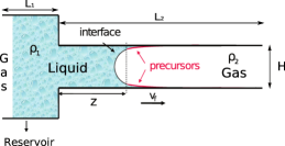
(b)

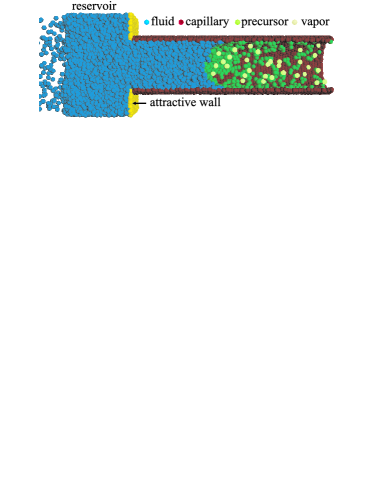
Figure 1: Sketch of the geometry used for the description of the capillary imbibition in the LB and MD simulations. (a) The 2 dimensional geometry, with length $L_{1}+L_{2}$ and width $H$, is divided in two parts. The left part has top and bottom periodic boundary conditions, so as to support a perfectly flat gas-liquid interface, mimicking an “infinite reservoir”. In the right half, of length $L_{2}$, there is the actual capillary: the top and bottom boundary conditions are solid wall, with a given contact angle $\theta$. Periodic boundary conditions are also imposed at the inlet and outlet sides. The main LB parameters are: $H\equiv ny=40,L_{2}=nz=170,\rho_{1}=1;\rho_{2}=0.35,\mu_{1}=0.66,\mu_{2}=0.014,\gamma=0.016$ where $H$ is the channel height, $L_{2}$ is the channel length, $\rho_{2}$ and $\rho_{1}$ the gas and liquid densities respectively: $\mu_{k}$, $k=1,2$ the dynamic viscosities, and $\gamma$ the surface tension. (b) Snapshot of fluid imbibition for MD in the capillary at time $t=1300$ MD time-steps. The fluid is in equilibrium with its vapour. Fluid atoms are in blue. Vapour is yellow, tube walls are red and the precursor is green. One distinguishes between vapour and precursor, subject to the radial distance of the respective atoms from the tube wall, if a certain particle has no contact with the wall, it is deemed ’vapour’. The MD parameters are as follows [42]: $R=11\sigma,L=80\sigma,\rho_{l}=0.774,~{}\mu=6.3,~{}\gamma=0.735,~{}\sigma=1$, where $R$ is the capillary radius and $L$ its length.

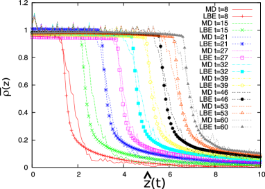
(a) (b)

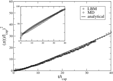
Figure 2: Dynamics of the bulk and precursor meniscus. (a) Position of the liquid meniscus $\hat{z}^{2}(t)$ for LB and MD simulations. The position of the precursor film, $\hat{z}^{2}_{prec}(t)$ is also plotted for both models. $\hat{z}_{prec}$ is defined as the rightmost location with density $\rho=\rho_{bulk}/3$. All quantities are given in natural “capillary” units (see text). The asymptotic ($t>15t_{cap}$) rise of both precursor and bulk menisci follows a $t^{1/2}$ law, with different prefactors (see the two straight lines), even though the underlying microscopic physics is different. Notably, the precursor film is found to proceed with the law: $\hat{z}^{2}_{prec}(t)=1.35\hat{t}$. (b) Profiles of the average fluid density $\overline{\rho}(z)$ in the capillary at various times for LB and MD models.

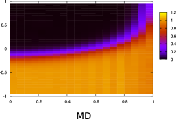
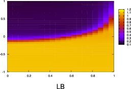
Figure 3: The two figures show the fluid density profile in the vicinity of the meniscus, LJ-MD (left) and LB (right), at time $\hat{t}=20$ The MD results are rescaled so that the width is the same for both methods.

Since binary LB methods do not easily support high density ratios between the two species, we impose the correct ratio between the two dynamic viscosities through an appropriate choice of the kinematic viscosities. The chosen parameters correspond to an average capillary number $Ca\approx 3\;10^{-2}$ and $Ca\sim 0.1$ for LB and MD respectively. In order to emphasise the universal character of the phenomenon and to match directly MD and LB profiles, results are presented in natural units, namely, space is measured in units of the capillary size, $l_{cap}$ and time in units of the capillary time $t_{cap}=l_{cap}/V_{cap}$, where $V_{cap}=\gamma/\mu$ is the capillary speed and $l_{cap}=H/C_{LB}$ for LB and $l_{cap}=R/C_{MD}$ for MD. The reduced variables are denoted as $\hat{z}$ and $\hat{t}$.

In figure 2a, we show $\overline{\rho}(z)$ at various instants (in capillary units), for both MD and LB simulations. Choosing a constant time-interval $\Delta\hat{t}=7$ between subsequent profiles, it is clear that the interface position advances slower than linearly with time. The relatively high average density $\overline{\rho}(z)$ near the wall witnesses the presence of a precursor film attached to the wall. Indeed, the profiles $\overline{\rho(z)}$ at late times become distinctly nonzero far ahead of the interface position (near the right wall at $\hat{z}\approx 10$ where the capillary ends), due to a fluid monolayer attached to the wall of the capillary: this precursor advances faster then the fluid meniscus in the pore center, but also with a $\sqrt{t}$ law (see below). From this figure, it is appreciated that quantitative agreement between MD and LB is found also between the spatial profiles of the density field. This is plausible, since the LB simulations operate on similar principles as the MD ones, namely the fluid-wall interactions are not expressed in terms of boundary conditions on the contact angle, like in continuum methods, but rather in terms of fluid-solid (pseudo)-potentials. In particular, the degree of hydrophob/philicity of the two species can be tuned independently, by choosing different values of the fluid-solid interaction strengths (for details see [42, 43]). In figure 2b, we show the position of the advancing front and the precursor film as a function of time, for both MD and LB simulations. Even though the average capillary numbers are not exactly the same, a pretty good agreement between LB and MD is observed. In particular, in both cases, the precursor is found to obey a $\sqrt{t}$ scaling in time, although with a larger prefactor than the front. As a result, the relative distance between the two keeps growing in time, with the precursors serving as a sort of ’carpet’, hiding the chemical structure of the wall to the advancing front. In spite of the different capillary number, the agreement between LB and MD can be attributed to the fact that these two approaches share the same static angle, $\theta_{0}=0$, since the “maximal film” [1], or complete wetting, configuration has been imposed by increasing the strength of the wall-fluid attraction [42, 43], i.e. imposing that the spreading coefficient $S>0$ [1].

In natural units, the Lucas-Washburn law takes a very simple universal form

$${\hat{z}}^{2}=\hat{z}_{0}^{2}+\hat{t}~{},$$ (15)

where we have inserted the value of $cos(\theta)=1$, corresponding to complete wetting. As to the bulk front position, fig.2a shows that both MD and LB results superpose with the law (15), while the precursor position develops a faster dynamics, fitted by the relation [18]:

$${\hat{z}}^{2}_{prec}=\hat{z}_{0}^{2}+1.35\hat{t}~{}.$$ (16)

Similar speed-up of the precursor has been reported also in different experimental and numerical situations [15, 44]. The precursor is here defined through the density profile, $\overline{\rho}(z)$, averaged over the direction across the channel.

In figure 3, we show a visual representation of the quantitative agreement between MD and LB dynamics: we present the density isocontour which can be imagined as the advancing front. It is seen that the interface positions are in good agreement and also density structures are very similar.

These results achieve the validation of the LB method against the MD simulations. Moreover, as recently pointed out [42, 41, 18], our findings indicate that hydrodynamics persists down to nanoscopic scales. The fact that the MD precursor dynamics quantitatively matches with mesoscopic simulations, suggests that the precursor physics also shows the same kind of nanoscopic persistence.

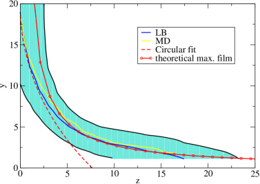
Figure 4: The extrapolated interface position for both methods and the theoretical profile for “maximal film”. The x- and y- axis are normalised in order to reproduce the LB units. The colored region represents the whole interface. It is delimited, on the left, by the solid line representing the isolines of the bulk density ($\rho=0.9$) and on the right by the one describing the beginning of the lighter fluid ($\rho=0.1$), where only few molecules of the penetrating fluid are present because of diffusion. The length of the precursor film appear in line with the relation $L_{p}=7.210^{-1}Ca^{-1}$ found in a recent nanoscale experiment [14].

Figure 5: Disjoining pressure in LB and its fit based upon analytical expression are shown versus the distance from wall. The analytical expression for Van der Waals forces is given by $\frac{A}{6\pi y^{3}}$, where is the Hamakar constant $A=\pi^{2}k\alpha_{l}(\alpha_{s}-\alpha_{L})$ and $\alpha_{s},\alpha_{L}$ are the polarizabilities of the solid and the liquid. In our case of total wetting, $A>0$ [2] and our data are fitted by using $A=0.019$.

Fig. 4 shows the whole interface in the vicinity of the meniscus and, in particular, the shape of the precursor computed with both methods. The plot emphasises the presence of a precursor film at the wall. The agreement between the two methods is again quantitative. The interface in both methods turns out to be about $5$ units. The precursor film profile, defined by the isoline of points with density $\rho=\rho_{bulk}/3$, is split in two regions. In the first that arrives until $y\approx 7$, it is fitted by a circular profile with center at $z_{0}=0,y_{0}=20$ and radius $r=18$. In the second, from $y\approx 7$ to the wall, the film is fitted by the function $\frac{a^{2}}{Caz}$. In this formula, $a$ is a characteristic molecular size which is taken to be $a=1$ in our case. This profile is obtained in the lubrication approximation considering Van der Waals interaction between fluid and walls [1], in the case of “maximal film” (perfect wetting). Quantitative agreement is again found between LB, MD and analytics, thus corroborating the idea of the Shan-Chen pseudo-potential as a quantitative proxy of attractive Van der Waals interactions in the low density regime, where hard-core repulsion can be neglected. It is interesting to note that the presence of the precursor film guarantees an apparent angle $\theta=0^{\circ}$,whereas the angle calculated from the circular fit of the bulk meniscus would be $\theta\approx 40^{\circ}$ Since these forces are, apparently, the key microscopic ingredient to be injected into an otherwise continuum framework, it is plausible to expect that LB should be capable of providing a realistic and quantitative description of precursor dynamics. The results of the present simulations confirm these expectations and turn them into quantitative evidence. We have also computed the disjoining pressure inside the film in order to corroborate the idea that LB is capable of correctly describing the dynamics of the precursor film. Such pressure is related to the chemical potential and it is function of the distance from walls, that is of the thickness of the film [2]. In fig. 5, the disjoining pressure computed inside the film in the LB is compared with the fit based upon the analytical expression given for Van-der-Waals forces. LB is a diffuse-interface model and, therefore, can not guarantee a pure hydrodynamical behaviour with ideal interfaces inside a thin film, such as the precursor film experienced in this work. Nevertheless, is seems to assure a disjoining pressure at least compatible with microscopic physics, with the correct divergence at the wall. This appears to be consistent with the fact that real interfaces are found to be diffuse also in experiments at macroscopic scales [15].

4.2 Nanochannel in presence of an obstacle

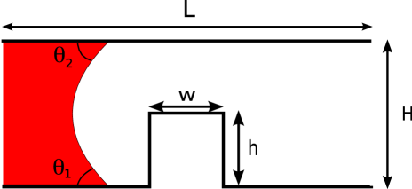
Figure 6: A channel of length $L=200$ LB units and width $H=41$ LB units is studied. The contact angles at the bottom and top walls are taken to be $\theta_{1}=\theta_{2}=\theta$. An square obstacle is also present, whose dimensions are given by the height $h$ and the width $w$.

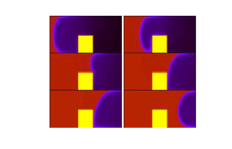
Figure 7: Snapshots of density at different times $t=20000,30000,40000,50000,60000,100000$ LB units.

(a)

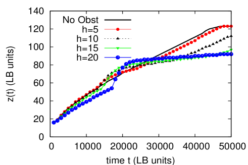
(b)

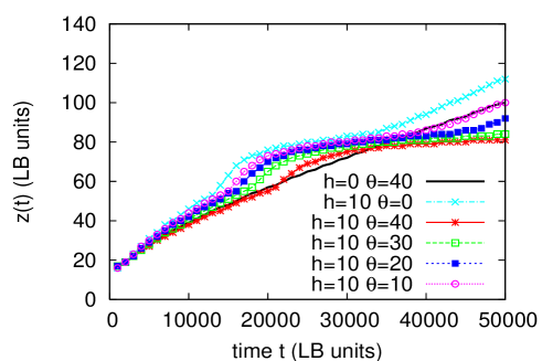
(c)

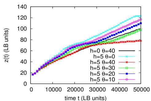
Figure 8: In all figures square obstacles (with width equal to the height) are considered and the front position versus time is shown. (a) Different obstacle height are considered for $\theta=0^{\circ}$. (b)The contact angle is changed (from 0 to 40 degrees) taking the height of the obstacle constant and equal to $h=10$. The front dynamics for the case with no obstacle and $\theta=40^{\circ}$ is also shown for comparison. (c) Same as in (b) but with $h=5$.

In this section, we study the capillary filling in a nano-channel in presence of an obstacle. In particular, we want to analyse the effect of the precursor films on the dynamics of the fluid when crossing the obstacle. This test-case has been simulated through the LB model and the geometry is depicted in figure 6. First, we simulate a channel with hydrophilic walls which support a complete wetting ($\theta=0^{\circ}$). An obstacle is put in the middle of the channel length with dimensions $w=h=20$ LB units. Six snapshots of the density evolution with time are represented in figure 7. Precursor films are visible ahead of the meniscus of the penetrating fluid at the bottom wall. Such film wets the obstacle before the front encounters it. The obstacle is large (its width is equal to the half of the channel) but the contact angle is small and therefore the front does not pin and is able to pass the obstacle in a relative short time, as known according to the Gibbs, or Concus-Finn, criterion [45, 46]. Nevertheless, the meniscus dynamics is deeply affected by the presence of the obstacle. It is seen that the liquid on the top wall advances much more rapidly than the one on the bottom wall. In particular, at the beginning and at the end of the obstacle the meniscus line is strongly distorted. After some time,

We now perform a systematic series of simulations, where we vary the height of the obstacle in order to check to what extent the dynamics is affected by wall roughness. In figure 8, the detailed characteristics of the front dynamics are analysed. In figure 8a, it is possible to appreciate that, for complete wetting $\theta=0^{\circ}$, the presence of a small obstacle ($h=5=H/8$) is negligible. The front advances almost in the same way for the cases $h=0^{\circ}$ and $h=5$. This is possibly due to the presence in these cases of precursor films which wet the obstacle anticipating the meniscus. In this way, they “hide” the roughness and let the front pass through the obstacle without feeling any roughness. For an obstacle of middle width $h=10$, the front is strongly distorted and slowed down but it recovers the initial slope, after it has passed through the obstacle. On the contrary, for larger obstacles $h\geq 15$ the dynamics of the meniscus seems to be irreversibly changed and it advances with a decreased slope after the obstacle. Then, we carry out numerical simulations keeping the height of the obstacle ($h=10$) constant, while varying the contact angle. In figure 8b, it is seen that the slope of the curve is strongly affected by the value of the contact angle and, notably, for $\theta>20^{\circ}$ the curve is not able to recover the initial dynamics but it results much slower. Moreover, the velocity of the advancing front is strongly decreased when the walls are not very hydrophilic and with roughness. For instance, the front advances very similarly for $\theta=40^{\circ}$ without roughness $h=0$ and for $h=10,\theta=10^{\circ}$. This seems to confirm the guess that the precursor films can reduce the drag in presence of roughness. In figure 8c, the same analysis is worked out for an obstacle with width $w=5$. The effect of such obstacle is quite small for $\theta<10^{\circ}$, where precursor films are supposed to be present. Naturally, it results increasingly important with the increase of the contact angle and it causes a change in slope for $\theta>30^{\circ}$.

5 Conclusions

Summarising, we have thoroughly analysed the capillary filling in a nanochannel by using atomistic and hydrokinetic methods.

We have reported quantitative evidence of the formation and the dynamics of precursor films in capillary filling with highly wettable boundaries. The precursor shape shows persistent deviation from an ideal circular meniscus, due to the nanoscopic distortion induced by the interactions with the walls. When properly scaled, the results do not seem sensitive to geometry (in this work we investigate two different geometries) and resolution. This has been connected to the disjoining pressure induced by Van der Waals interactions between fluid and solid and approximated in the LB approach by a suitable phenomenological model. Our findings are supported by direct comparison between LB, MD simulations and theoretical predictions, which suggests that a continuum description (LB) together with a proper inclusion of the solid-fluid interaction is able to reproduce this phenomenon. In this sense, this work provides a complete assessment of the LB method for the study of nanochannel capillary filling.

Then, a nanochannel with a square obstacle has been simulated via the LB model. The complete parametric analysis points out that for highly wetting walls ($\theta<10^{\circ}$) the presence of precursor films make the presence of small obstacles (with a width smaller than 1/8 of the channel height) negligible. Furthermore, results seems to indicate that to reach high flow rate it is preferable to choose very hydrophilic and rough walls rather than to use very smooth but hydrophobic walls.

3-D simulations will be carried out in order to assess these affirmations and to evaluate the effect of different obstacle geometry and position.

6 acknowledgments

S. Chibbaro’s work is supported by a ERG EU grant. This work makes use of results produced by the PI2S2 Project managed by the Consorzio COMETA, a project co-funded by the Italian Ministry of University and Research (MIUR). He greatly acknowledges the financial support given also by the consortium SCIRE. More information is available at http://www.consorzio-cometa.it. Work performed under the NMP-031980 EC project (INFLUS).

References

- [1] P. G. de Gennes, Rev. Mod. Phys. 57, 827 (1985)
- [2] P. G. de Gennes, F. Brochard-Wyart, and D. Quéré, Bubbles, Pearls, Waves (Springer, 2003).
- [3] B. Bhushan, J.N. Israelachvili, U. Landman, Nature 374, 607 (1995).
- [4] B. Zhao, J.S. Moore, and D.J. Beebe, Surface-directed liquid flow inside microchannels, Science 291, 1023 (2001).
- [5] G. Whitesides and A. D. Stroock, Flexible methods for microfluidics, Phys. Today 54, No. 6, 42 (2001).
- [6] A. D. Stroock et. al., Science 295, 647 (2002).
- [7] G. Martic et al., A Molecular Dynamics Simulation of Capillary Imbibition Langmuir 18, 7971, (2002).
- [8] S. Supple and N. Quirke, Phys. Rev. Lett., 90, 214501, (2003).
- [9] L.-J. Yang, T.J. Yao, and Y.-C. Tai, The marching velocity of the capillary meniscus in a microchannel, J. Micromech. Microeng., 14, 220, (2004).
- [10] W. Juang, Q. Lui, and Y. Li, Chem. Eng. Technol., 29, 716, (2006).
- [11] D. M. Karabacak, V. Yakhot, and K. L. Ekinci, Phys. Rev. Lett. 98, 254505 (2007).
- [12] P. Joseph et. al., Phys. Rev. Lett. 97, 156104 (2006).
- [13] D. Bonn, J. Eggers, J. Indekeu, J. Meunier, E. Rolley, Rev. Mod. Phys to appear.
- [14] H. Pirouz Kavehpour, Ben Ovryn, and Gareth H. McKinley, Phys. Rev. Lett. 91, 196104 (2003).
- [15] J. Bico, and D. Quéré Europhys. Lett. 61, 348 (2003).
- [16] T.D. Blake, and J. De Coninck Advances in Colloid and Interface Science 96, 21 (2002).
- [17] F. Heslot, A.M. Cazabat, and P. Levinson Phys. Rev. Lett. 62, 1286 (1989).
- [18] S. Chibbaro, L. Biferale, K. Binder, D. Dimitrov, F. Diotallevi, A. Milchev, S. Succi, S. Girardo, D. Pisignano Europhys. Lett. to appear (2008).
- [19] H. Kusumaatmaja, C. M. Pooley, S. Girardo, D. Pisignano, and J. M. Yeomans, Phys Rev E 77, 067301 (2008).
- [20] J. Ou, B. Perot, and Jonathan P. Rothstein, Phys Fluids 16, 12 (2004).
- [21] J. Hyvaluoma and J. Harting, Phys. Rev. Lett 100, 246001 (2008).
- [22] P.A. Thompson, and S.M. Troian, A general boundary condition for liquid flow at solid surfaces Nature, 389, 360, (1997).
- [23] S. Reddy, P.R. Schunk, R.T. Bonnecaze, Phys of Fluids 17, 122104 (2005).
- [24] M.P. Allen and D.J. Tildesley, ”Computer Simulation of Liquids”, Clarendon Press, Oxford (1987); D. Rapaport, ”The Art of Molecular Dynamic Simulations”, Cambridge University Press, Cambridge (1995).
- [25] R. Benzi, S. Succi, and Vergassola, Phys. Rep. 222, 145, (1992).
- [26] D.A. Wolf-Gladrow Lattice-gas Cellular Automata and Lattice Boltzmann Models (Springer, Berlin, 2000).
- [27] J. Horbach, and S. Succi, Phys. Rev. Lett. 96, 224503 (2006).
- [28] M. Sbragaglia,R. Benzi, L. Biferale, S. Succi, and F. Toschi, Phys. Rev. Lett. 97 (2006) 204503.
- [29] M.R Swift, W.R. Osborn, J.M. Yeomans, Phys. Rev. Lett. 75 (1995) 830.
- [30] J. Harting, C. Kunert, H.J. Herrmann, Europhys. Lett. 75 (2006) 328.
- [31] S. Cottin-Bizonne J.L. Barrat, L. Bocquet, E. Charlaix Nat. Mater. 2, 237-240 (2003).
- [32] N.R. Tas et al., Appl. Phys. Lett. 85, 3274, (2004).
- [33] X. Shan, and H. Chen, Phys Rev E 47, 1815, (1993). X. Shan, and G. Doolen, J. Stat. Phys. 81, 1-2, (1995).
- [34] Q. Kang, D. Zhang and S. Chen, Phys. Fluids 14 (9) 3203, (2002)
- [35] R. Benzi, L. Biferale, M. Sbragaglia, S. Succi, and F. Toschi, Phys. Rev. E 74 (2006) 021509.
- [36] H. Huang, D. T. Thorne, M. G. Schaap, and M. C. Sukop, Phys. Rev. E 76, 066701 (2007).
- [37] T. Soddemann, B. Dünweg, and K. Kremer, ”Dissipative particle dynamics: A useful thermostat for equilibrium and nonequilibrium molecular dynamics simulations”, Phys. Rev. E, 68, 046702 (2003).
- [38] P.J. Hoogerbrugge and J.M.V.A. Koelmann, ”Simulating microscopic hydrodynamic phenomena with dissipative particle dynamics”, Europhys. Lett. 19, 155 (1992); P. Espanol, ”Hydrodynamics from dissipative particle dynamics”, Phys. Rev. E 52, 1734 (1995).
- [39] E.W. Washburn, Phys. Rev. 27 (1921) 273.
- [40] R. Lucas, Kolloid-Z 23 (1918) 15.
- [41] P. Huber, K. Knorr, and A.V. Kityk, Mater. Res. Soc. Symp. Proc. 899E, N7.1 (2006).
- [42] D. I. Dimitrov, A. Milchev, and K. Binder, Phys. Rev. Lett. 99, 054501 (2007)
- [43] S. Chibbaro, The European Physical Journal E 27 01 (2008).
- [44] Popescu, S Dietrich, and G Oshanin, J. Phys.: Condens. Matter 17 4189 (2005)
- [45] P. Concus and R. Finn, On the behavior of a capillary surface in a wedge, Appl. Math. Sci., 63, 292(1969); P. CONCUS, and R. FINN, On Capillary Free Surfaces in the Absence of Gravity, Acta Math. 132, 177(1974); R. FINN, Existence and Non-existence of Capillary surfaces, Manuscripta Math. 28, 1(1979).
- [46] J. W. Gibbs, in Scientiic papers 1906, Dover, New York, 1961.