On the analogy between streamlined magnetic and solid obstacles

Abstract

Analogies are elaborated in the qualitative description of two systems: the magnetohydrodynamic (MHD) flow moving through a region where an external local magnetic field (magnetic obstacle) is applied, and the ordinary hydrodynamic flow around a solid obstacle. The former problem is of interest both practically and theoretically, and the latter one is a classical problem being well understood in ordinary hydrodynamics. The first analogy is the formation in the MHD flow of an impenetrable region – core of the magnetic obstacle – as the interaction parameter $N$, i.e. strength of the applied magnetic field, increases significantly. The core of the magnetic obstacle is streamlined both by the upstream flow and by the induced cross stream electric currents, like a foreign insulated insertion placed inside the ordinary hydrodynamic flow. In the core, closed streamlines of the mass flow resemble contour lines of electric potential, while closed streamlines of the electric current resemble contour lines of pressure. The second analogy is the breaking away of attached vortices from the recirculation pattern produced by the magnetic obstacle when the Reynolds number $Re$, i.e. velocity of the upstream flow, is larger than a critical value. This breaking away of vortices from the magnetic obstacle is similar to that occurring past a solid obstacle. Depending on the inlet and/or initial conditions, the observed vortex shedding can be either symmetric or asymmetric.

Introduction

External magnetic fields are heavily exploited in many practical applications Davidson:Review:1999 , such as electromagnetic stirring, electromagnetic brakes, and non-contact flow measurements Thess:Votyakov:Kolesnikov:2006 . The crucial aspect in the above applications is the Lorentz force produced by the interaction of an external magnetic field with induced electric currents. The currents appear because an electrically conducting fluid moves relative to the external field. The Lorentz force has a double effect on the flow: it suppresses turbulent fluctuations when the intensity of the external field is strong and spatially uniform, but also is able to produce vorticity if the intensity varies spatially. If the external magnetic field is localized in space, i.e. it acts on a finite region of flow, then the flow is decelerated in this region and one can say that the local magnetic field produces a virtual obstacle, called a magnetic obstacle. Both a solid and magnetic obstacle have a real physical effect in the sense that they impede the flow.

The retarding effect of the external nonuniform magnetic field on the liquid metal flow is well-known and has been intensively studied in the past, see for instance books Tananaev:book:1979 ; Moreau:book:1990 ; Davidson:book:2001 ; Mueller:Buehler:Book:2001 . The overwhelming majority of works were performed on liquid metal flows in ducts subject to fringing magnetic fields. The main goal was to study the so-called M-shaped velocity profile formed by directing the flow into the region of the fringing magnetic field. The M-shaped profile is characterized by two side jets around a central stagnant region.

The flow around a solid obstacle, such as a circular cylinder schematically given in Fig. 1($a$), is a classical hydrodynamical problem that is qualitatively well understood. The structure of the wake of the cylinder depends on the Reynolds parameter $Re=u_{0}d/\nu$, where $u_{0}$ is velocity at infinity, $d$ is the cylinder diameter, and $\nu$ the kinematic viscosity of the fluid. Physically, $Re$ expresses the ratio of inertial to viscous forces. When the inertia of the flow increases, two attached vortices appear past the cylinder, Fig. 1($b$). As the inertia of the flow increases further, the vortices detach from the cylinder and form the von Karman vortex street.

The flow around a magnetic obstacle like those schematically given in Fig. 1($c$) is a rather new MHD problem that is not yet completely understood. The first studies devoted to liquid metal flow around a magnetic obstacle were carried out in the former Soviet UnionGelfgat:Peterson:Sherbinin:1978 ; Gelfgat:Olshanskii:1978 . 2D numerical calculations Gelfgat:Peterson:Sherbinin:1978 have found two vortices inside the magnetic obstacle, however, especially designed experiments Gelfgat:Olshanskii:1978 did not confirm the numerical finding. Lately the term ‘magnetic obstacle’ has been revived for Western readers in 2D numerical works Cuevas:Smolentsev:Abdou:Pamir:2005 ; Cuevas:Smolentsev:Abdou:PRE:2006 ; Cuevas:Smolentsev:Abdou:2006 , where authors also have found a vortex dipole in a creeping MHD flow Cuevas:Smolentsev:Abdou:PRE:2006 and claimed that vortex generation past a magnetic obstacle is similar to that past a solid obstacle Cuevas:Smolentsev:Abdou:2006 .

The most recent results for the flow around a magnetic obstacle were obtained by means of 3D numerics and physical experiments Votyakov:PRL:2007 ; Votyakov:JFM:2007 . It turns out that the structure of the wake of the magnetic obstacle is more complex that that of the solid obstacle. In addition to the Reynolds number, $Re=u_{0}\,H/\nu$, an MHD flow is characterized by the magnetic interaction parameter, $N=\sigma H\,B_{0}^{2}/\rho u_{0}$, where $H$, $u_{0}$, $B_{0}$ are the characteristic length scale, velocity and intensity of the applied magnetic field, and $\rho$ and $\sigma$ are the density and electric conductivity of the fluid, see e.g. Shercliff:book:1962 ; Roberts:1967 ; Moreau:book:1990 ; Davidson:book:2001 . $N$ represents the ratio of the Lorentz force to the inertial force. Depending on $Re$ and $N$, i.e. on the relationship between viscous, Lorentz and inertial forces, the liquid metal flow shows three different regimes: (1) no vortices, when the viscous force prevails at the small Lorentz force limit, (2) one pair of magnetic vortices when Lorentz force is high and inertia is small, and (3) three pairs (namely, magnetic, connecting, and attached vortices) when the Lorentz and inertial forces dominate the viscous force. The latter case is shown in Fig. 1$d$. We believe that this scenario for the wake of the magnetic obstacle is the generic one and devote the last Section of the paper to explain in detail why this is so.

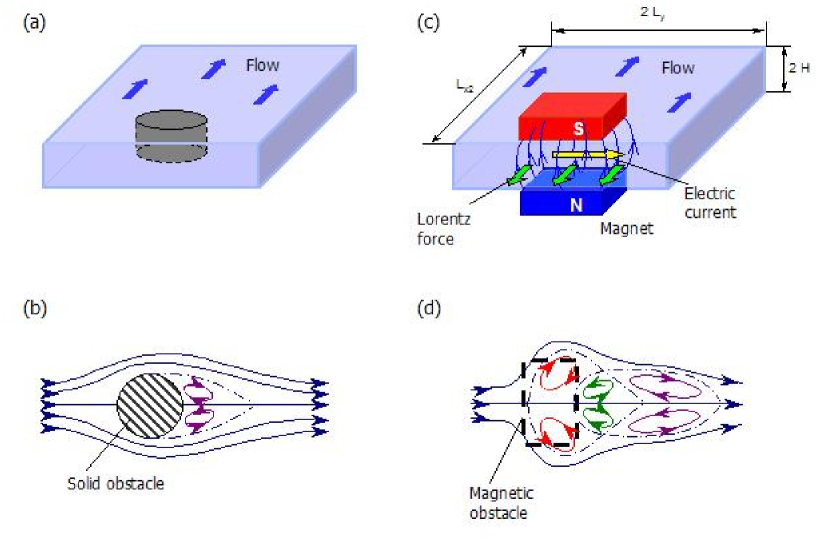
Figure 1: Flow around a solid ($a,b$) and magnetic ($c,d$) obstacle. Wake of the solid obstacle ($b$) shows two attached vortices, wake of the magnetic obstacle ($d$) shows inner magnetic (first),connecting (second) and attached vortices (third pair).

An analogy between solid and magnetic obstacles had been suggested from the beginning of MHD liquid metal works in the former USSR . Based on 2D inertialess simulations, Gelfgat et al. Gelfgat:Peterson:Sherbinin:1978 remarked that a vortex dipole inside the magnetic obstacle is similar to attached vortices past a solid obstacle. Afterwards, a series of experiments of Gelfgat et al. Gelfgat:Olshanskii:1978 failed to confirm the numerical results and this let them to question the original suggestion. As has been shown recently Votyakov:PRL:2007 , however, the problem with the suggested analogy is that the numerically observed flow structures were magnetic vortices fixed inside the magnetic obstacle rather than the attached vortices disposed past the magnetic obstacle. The 2D numerical results Gelfgat:Peterson:Sherbinin:1978 were correct for creeping flow, while the physical experiments Gelfgat:Olshanskii:1978 were performed at high Reynolds numbers $Re$, and so they failed to produce any vortices since the interaction parameter $N$ was not high enough Votyakov:JFM:2007 .

Then, Cuevas et al. Cuevas:Smolentsev:Abdou:Pamir:2005 ; Cuevas:Smolentsev:Abdou:2006 , by means of 2D and quasi-2D numerics , concluded that the vortex generation past a magnetic obstacle is similar to that past a solid cylinder. Although this conclusion is correct in general, it is rather obvious: any decelerating force generates vorticity that is then translated downstream, exciting in the process the von Karman vortex street. Moreover, at high Reynolds numbers, 2D numerics is not a suitable method to analyze the flow around the magnetic obstacle because it neglects the Hartmann friction Votyakov:JFM:2007 , and as a result, fails to describe the stable six-vortex structure shown in Fig. 1$d$ and discussed later.

The possible reason why the previous two analogies were either imprecise Gelfgat:Peterson:Sherbinin:1978 or trivially correct Cuevas:Smolentsev:Abdou:2006 is because the previous interpretations were not based on full 3D numerical simulations at high Reynolds numbers. As a result, the previous interpretations suffered from the lack of a concrete and clear demonstration. The basic message of our paper is to report the correct, in our opinion, analogy, and to confirm it by means of concrete 3D numerical results.

A fruitful way of thinking about the similarity between magnetic and solid obstacles is that the magnetic and connecting vortices, taken together as one entity, form the body of a virtual insertion in the MHD flow Votyakov:PRL:2007 . One can understand it by recalling the classical potential flow theory. In this theory, a real streamlined cylinder is modelled by a virtual imaginable vortex dipole. In the MHD case, we have an opposite picture: a magnetic obstacle, that can be understood as a virtual bluff body, manifests itself by means of real physical vortices. The present paper supports this idea with two new aspects.

The first is the impenetrable core of the magnetic obstacle. It originates in the center of the magnetic gap as the magnetic interaction parameter $N$ increases. When $N$ is very large, both mass transfer and electric field vanish in the region between magnetic poles. This region looks as if frozen by the external magnetic field so that the upstream flow and crosswise electric currents can not penetrate inside it. Thus, the core of the magnetic obstacle is similar to an insulated solid obstacle inside an ordinary hydrodynamical flow with crosswise electric currents and without an external magnetic field. In this latter case, because of the absence of a magnetic field, the crosswise electric currents go around the insulated insertion without affecting the mass flow. Magnetic vortices are located aside the core and compensate shear stresses, like a ball-bearing between the impenetrable region and upstream flow.

At first glance, the appearance of the core of the magnetic obstacle can be admitted as intensively studied before. Indeed, a stagnant region between two side jets is well-known for duct flows subject to fringing magnetic fields. However, at a closer examination one finds that the fringing magnetic field is not the case of the magnetic obstacle. In the former case, the side jets of the M-shaped velocity profile are caused by a geometrical heterogeneity imposed by the sidewalls of the duct, so the stagnant region tends to spread between the sidewalls. In the latter case, maxima of streamwise velocity appear in an originally free flow around the region where the magnetic field is of highest intensity, and the core roughly corresponds to the region where the magnetic field is imposed.

To our knowledge, most of numerical studies of fringing magnetic fields were performed with the 2D assumptions, i.e. the flow was treated as quasi 2D, where only the transverse field component ($B_{z}$) was taken into consideration, while the other components ($B_{x}$ and $B_{y}$) were neglected. As a result, the studied magnetic field was inconsistent, that is, the requirements for the field to be curl- and divergence-free were violated Votyakov:TCFD:2009 . So, this is one of the contributions of the present work: a complete systematic 3D numerical study with $N$ changing smoothly from low to high, while maintaining a physically consistent curl- and divergence-free external magnetic field.

A new physical effect compared to the fringing magnetic fields is a neat demonstration of the vortices alongside the stagnant core. It has been shown recently that the spanwise homogeneous fringing magnetic field does not enable any recirculation Votyakov:JFM:2007 .

The second aspect of the paper is the detachment of the vortices from the magnetic obstacle when the Reynolds number $Re$ is large enough. Magnetic and connecting vortices are in rest during the vortex shedding. The shedding can be either symmetric, in which both attached vortices are coming off simultaneously, or asymmetric, as it usually happens with a solid obstacle when $Re$ exceeds a critical value. The symmetric vortex shedding is also possible in an ordinary hydrodynamic flow past an infinitely long cylinder that is specially perturbed to provoke the synchronous vortex shedding, see e.g. Konstantinidis:Balabani:2007 .

The presented results are complementary to those published in Votyakov:PRL:2007 ; Votyakov:JFM:2007 . They were unavailable before because there required extensive sets of 3D numerical simulations: a series of runs for large $N$ to refine the core of the magnetic obstacle, and a series of runs involving long time integrations to produce laminar time-periodic vortex shedding at high $Re$. Each of these sets of runs is discussed below in its own section.

The structure of the present paper is as follows. First, we present technical details of the simulations: model, equations and 3D numerical solver. Then, we report results for the core of the magnetic obstacle and demonstrate possible symmetric and asymmetric vortex shedding in the wake past the obstacle. The last Section before the Summary explains the generic scenario for the wake of the magnetic obstacle and the similarities with the vortex shedding past the solid obstacle. A summary of the main conclusions ends the paper.

Model, equations, numerical method

A schematic of the model is shown in Fig. 1($c$). It is the same as detailed in Votyakov:JFM:2007 except for the fact that, in the present case, we have no side walls. Instead, here we use slip boundary conditions in the crosswise direction, and therefore, expand the crosswise dimension of the computational domain. Also, in vortex shedding simulations, we double the outlet length compared to Votyakov:JFM:2007 in order to exclude the outlet influence on the vortex detachment and advection.

The governing equations for an electrically conducting and incompressible fluid, subject to an external magnetic field, are the Navier-Stokes equations coupled with the Maxwell equations for a moving medium and Ohm’s law. Here, the magnetic Reynolds number $R_{m}=\mu^{*}{\sigma}u_{0}H$ is supposed to be much less than one, where, $\mu^{*}$ is the magnetic permeability. This corresponds to the so called quasi-static (or inductionless) approximation, where it is assumed that the induced magnetic field is infinitely small in comparison to the external magnetic field, see, e.g. Roberts:1967 . The resulting equations in dimensionless form are:

$$\frac{{\partial\textbf{u}}}{{\partial t}}+(\textbf{u}\cdot\nabla)\textbf{u} = -\nabla p+\frac{1}{Re}\triangle\textbf{u}+N(\textbf{j}\times\textbf{B}),\;\;\;\nabla\cdot\textbf{u}=0,$$ (1)

j $$= -\nabla\phi+\textbf{u}\times\textbf{B},\;\;\;\;\nabla\cdot\textbf{j}=0,$$ (2)

where $\bf{u}$ denotes velocity field, $\bf{B}$ is the external magnetic field, $\bf{j}$ is the electric current density, $p$ is the pressure, and $\phi$ is the electric potential. The interaction parameter $N$ and Reynolds number $Re$, $N=Ha^{2}/Re$, are linked by means of the Hartmann number: $Ha=HB_{0}(\sigma/\rho\nu)^{1/2}$. The Hartmann number determines the thickness of the Hartmann boundary layers, $\delta/H\sim Ha^{-1}$ for flow under constant magnetic field.

The origin of the coordinate system is taken in the center of the magnetic gap. The computational domain is: $-L_{x1}\leq x\leq L_{x2}$, $-L_{y}\leq y\leq L_{y}$, $-H\leq z\leq H$, where $x,y,z$ are respectively the streamwise, crosswise, and transverse directions, and $L_{x1}$ ($L_{x2}$), $L_{y}$, and $H$ are the inlet (outlet), crosswise, and transverse dimensions of the simulation box. $L_{x2}=25$ in runs for the core of the magnetic obstacle, and $L_{x2}=50$ in runs for vortex shedding; $L_{x1}=25$, $L_{y}=25$, $H=1$ in both simulations. Magnetic poles are located at $x=0$, $y=0$, $z=\pm h$, and the size of the magnet is $|x|\leq M_{x}$, $|y|\leq M_{y}$, $|z|\geq h$. The intensity of the external magnetic field ${\bf B(r)}$ is calculated by means of formulae given in Votyakov:JFM:2007 with $M_{x}=1.5$, $M_{y}=2$, and $h=1.5$. Different cuts of the intensity ${\bf B(r)}$ for these parameters are plotted in Fig. 3 and Fig. 4($b$) in paper Votyakov:JFM:2007 .

The characteristic dimensions for the Reynolds number $Re$, and the interaction parameter $N$ are the half-height of the duct $H$, the mean flow rate $u_{0}$, and the magnetic field intensity $B_{0}$, taken at the center of the magnetic gap, $x\!=\!y\!=\!z\!=\!0$. So, all the distances $L_{x},L_{x1},L_{x2},L_{y},M_{y},M_{x},h$ are normalized by $H$; the velocity $\mathbf{u}$ by $u_{0}$; the magnetic field $\mathbf{B}$ by $B_{0}$; the electric current density $\mathbf{j}$ by $\sigma u_{0}B_{0}$; the electric potential by $Hu_{0}B_{0}$; the pressure $p$ by $\rho\nu u_{0}/H$.

For a given external field ${\bf B}(x,y,z)$, the unknowns of the partial differential equations (1 – 2) are the velocity vector field ${\bf u}(x,y,z)$, and two scalar fields: the pressure $p(x,y,z)$ and the electric potential $\phi(x,y,z)$. To find the unknowns we use a finite differences method that was implemented in a 3D numerical solver as been detailed inVotyakov:Zienicke:FDMP:2006 . The solver was developed from a free hydrodynamic solver created originally in the research group of Prof. M. Griebel (Griebel:book:1995 ). The solver employs the Chorin-type projection algorithm and finite differences on an inhomogeneous staggered regular grid. Time integration is done by the explicit Adams-Bashforth method that has second order accuracy. Convective and diffusive terms are implemented by means of the VONOS (variable-order non-oscillatory scheme) method. The 3D Poisson equations are solved for pressure and electric potential at each time step by using the bi-conjugate gradient stabilized method (BiCGStab).

To complete the numerical model, boundary conditions have to be specified. No slip and insulating walls were specified in the transverse direction, while slip walls were used in the crosswise direction. In order to test the effect of boundary conditions, in some of the runs carried out for the core of the magnetic obstacle, the slip conditions in the crosswise direction were replaced by periodic boundary conditions. However, changing the crosswise boundary conditions was found to have no effect on the structure of the core. This is because $L_{y}=25$ is large enough compared to $M_{y}=2$ in all the runs for the core.

The outlet of the computational domain was treated as a force-free (straight-out) border for the velocity. The electric potential at the inlet and outlet boundaries was taken to be equal to zero because the inlet and outlet are sufficiently far from the region of magnetic field. At the inlet, a 2D parabolic (Poiseuille) velocity profile was used that was uniform in the crossflow (spanwise) direction. In runs for the asymmetric vortex shedding, this profile was slightly perturbed in the crosswise direction at initial times and then kept symmetric and constant in time. The initial perturbation initiated the asymmetric vortex shedding and the followed symmetry and constancy assured that the asymmetric vortex shedding is independent of the inlet conditions.

Time integration in the runs for the core of the magnetic obstacles was carried out until a stationary laminar solution has been reached. In all these simulations, we found the same laminar solution at a given $Re$ and $N$ pair, independently of initial conditions. So, as initial conditions for runs corresponding to new $Re$ and $N$ we used 3D fields of velocity, pressure, and electric potential obtained from the previous runs having the closest $Re$ and $N$ values.

Time integration in the runs for the vortex shedding was continued until a time-periodic laminar solution was reached. These simulations were dependent on the initial conditions. We found two classes of solutions: symmetric and asymmetric distribution of attached vortices in the wake at large times. The details about the initial and inlet conditions for both cases are given in the beginning of the corresponding sections.

The simulation box has been discretized by an inhomogeneous regular 3D grid depending on the solved problem. Details about the numerical grid are given at the beginning of the corresponding sections.

Core of the magnetic obstacle

In this series of simulations, we focus on the flow around a magnetic obstacle at large interaction parameter $N$. In order to achieve large $N=Ha^{2}/Re$, the simulations were started at a small interaction parameter and $Ha$ was smoothly increased, while keeping $Re$ constant. Two values of the Reynolds number were studied, $Re=10\mbox{ and }100$, and no principal differences were found at the same $N$. These low values of $Re$ imply low inertial forces, therefore, only “two-vortex” patterns were produced, without connecting or attached vortices.

The numerical grid was regular and inhomogeneous, $N_{x}\times N_{y}\times N_{z}=64^{3}$. The minimal horizontal step size in the region of the magnetic gap was $\Delta x\simeq\Delta y\simeq 0.3$, which means that a few dozens points were used for resolving the inner vortices in the core of the magnetic obstacle. The minimal vertical step size near the top and bottom (Hartmann) walls was $\Delta z=0.005$. This corresponds to using three to five ($=(1/Ha)/\Delta z)$ points to resolve Hartmann layer at $Ha=40-70$.

The easiest way to understand the core of the magnetic obstacle is to analyze crosswise cuts through the center of the magnetic gap at different arising magnetic interaction parameters $N$. These cuts are shown in Fig. 2a for the streamwise velocity $u_{x}(y)$ and in Fig. 2b for the electric potential $\phi(y)$. First we discuss how the streamwise velocity changes as $N$ increases.

Because $N$ expresses the strength of the retarding Lorentz force relative to the inertial force, curve 1 in Fig. 2$a$ ($N=0.1$) is only slightly disturbed with respect to a constant. As $N$ increases, the curves $u_{x}(y)$ pull further down in the central part $u_{center}\doteqdot u_{x}(0)$, see for example curves 2 and 3. At $N$ higher than a critical value $N_{c,m}$, i.e. for curve 4, the central velocities $u_{center}$ are negative. This means that there appears a reverse flow causing magnetic vortices in the magnetic gap. When $N$ rises even more (see curves 5 and 6) the magnetic vortices become stronger and simultaneously shift away from the center to the side along the $y$ direction, see insertion in Fig. 2$a$ for curves 5 and 6.

The fact that the centerline velocity in the center of the magnetic gap goes to zero as $N$ increases is expected and was discussed earlier for fringing magnetic fields. In this respect, the case of the magnetic obstacle is analogous to the fringing magnetic field. What is different in these two cases is that the centerline velocity becomes negative before it goes to zero while this could not be so, and was never actually observed, for the fringing field Votyakov:JFM:2007 .

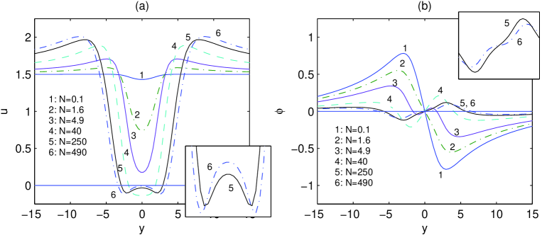
Figure 2: Streamwise velocity ($a$) and electric potential ($b$) along crosswise cuts of middle horizontal plane $x=z=0$. $Re=10$, $N=$0.1(solid 1), 1.6(dot-dashed 2), 4.9(solid 3), 40(dashed 4), 250(solid 5), and 490(dot-dashed 6). Insertion shows magnified plots for curves 5 and 6.

Fig. 2($b$) shows how the electric potential $\phi(y)$ varies along the central crosswise cut through the magnetic gap. The slope in the central point is the crosswise electric field, $E_{y,center}=-d\phi/dy|_{y=0}$. One can see that $E_{y,center}$ changes its sign: it is positive at small $N$ and negative at high $N$. To explain why it is so, one can use the following way of thinking. Any free flow tends to pass over an obstacle in such a way so as to perform the lowest possible mechanical work, i.e. flow streamlines are the lines of least resistance to the transfer of mass. The resistance of the flow subject to an external magnetic field is caused by the retarding Lorentz force $F_{x}\approx j_{y}B_{z}$, so the flow tends to produce a crosswise electric current, $j_{y}$, as low as possible while preserving the divergence-free condition $\nabla\cdot{\bf j}=0$. To satisfy the latter requirement, an electric field ${\bf E}$ must appear, which is directed in such a way, so as to compensate the currents produced by the electromotive force ${\bf u}\times{\bf B}$. Next, we analyze the crosswise electric current $j_{y}=E_{y}+(u_{z}B_{x}-u_{x}B_{z})$. Due to symmetry in the center of the magnetic gap $B_{y}=B_{x}=u_{y}=u_{z}=j_{y}=j_{z}=0$ so $j_{y}=E_{y}-u_{x}B_{z}$. This means that $E_{y}$ tends to have the same sign as $u_{x}$ in order to make $j_{y}$ smaller. At small $N$, the streamwise velocity $u_{x}$ is large and positive, so the electric field $E_{y}$ is positive too. When the magnetic vortices appear, there is a reverse flow in the center. Therefore, the central velocity is negative now, and the central electric field $E_{y,center}$ is also negative.

In Votyakov:JFM:2007 the change of the electric field in the magnetic gap is explained in terms of the Poisson equation and the concurrence between external and internal vorticity. This argument is also valid here, however in contrast to Votyakov:JFM:2007 , we have no side walls, so the external vorticity in the present case plays only a minor role. As a result, the reversal of the electric field appears at a small $N$ (approximately equal to five), which is close to the critical interaction parameter $N$ at $\kappa=0.4$ given in Votyakov:JFM:2007 . (In Votyakov:JFM:2007 , $\kappa$ is the ratio of the magnet width to the duct width.)

The overall data about $u_{center}$ and $E_{y,center}$ in the whole range of studied $N$ are shown in Fig. 3. One can see that both characteristics start from positive values, then, they cross the zeroth level, reach a minimum, go up again, and finally vanish in the limit of high $N$. With respect to the streamwise velocity, this means that, at hight $N$, there is no mass flow in the center of the magnetic gap; the other velocity components are equal to zero due to symmetry. With respect to the crosswise electric field, this means that there are no electric currents. This occurs because there is no mass flow, therefore, the electromotive force vanishes, $E_{y}$ goes to zero, and the other electric field components are equal to zero due to symmetry. Thus, one can say that the center of the magnetic gap is frozen by the strong external magnetic field, so that both mass flow and electric currents tend to bypass the center. In other words, this means that a strong magnetic obstacle has a core, and such a core is like a solid insulated body, being impenetrable for the external mass and electric charge flow.

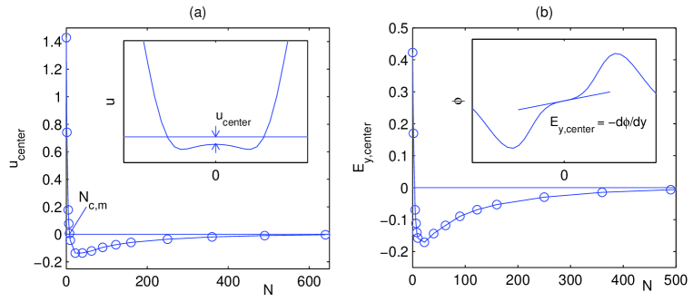
Figure 3: Central streamwise velocity $u_{center}$ ($a$) and central spanwise electric field $E_{y,center}$ ($b$) as a function of the interaction parameter $N$. $N_{c,m}$ is a critical value where the streamwise velocity is equal to zero. Insertion shows the definition of $u_{center}$ and $E_{y,center}$.

In the 2D creeping flow around the magnetic obstacle, the $u_{center}$ and $E_{y,center}$ vanishing behavior shown in Fig. 3 is impossible because it violates the flow continuity. At very high $N$ and low $Re$, instead of the frozen core obtained in the 3D case, a 2D flow develops various recirculation patterns in the core, because the secondary flow of the 3D magnetic vortices is forbidden in the 2D case. Paradoxically, the 2D creeping flow discussed in the paper by Cuevas et al. Cuevas:Smolentsev:Abdou:PRE:2006 is turned out to be more rich than the presented 3D creeping flow between two no-slip endplates. This point is discussed further in the last Section devoted to the generic scenario of the wake of the magnetic obstacle.

It is convenient to visualize the core of the magnetic obstacle by plotting streamlines for the mass flow, (see Fig. 4$a$) and electric charge transfer (see Fig. 4$b$) in the middle horizontal plane. One can see that the side streamlines envelop the bold dashed rectangle. This rectangle denotes the borders of the external magnet. Alongside the rectangle there are closed streamlines for mass flow (plot $a$), which are magnetic vortices. At high $N$, these vortices are located in the region of crosswise gradients of the external magnetic field and compensate shear stresses between the core of the magnetic obstacle and rest of the flow. Also, the magnetic vortices produce closed electric currents inside the rectangle (plot $b$). These internal currents are elongated in the $y$ direction. They are very weak compared to the external currents enveloping the obstacle.

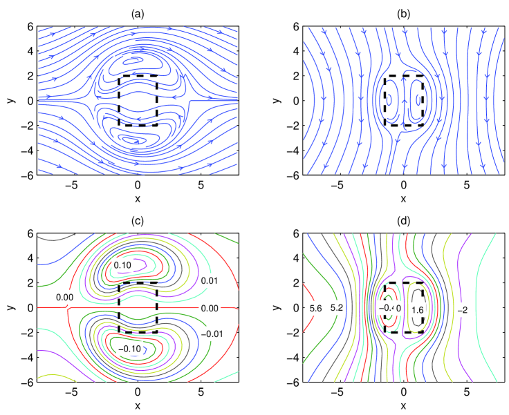
Figure 4: Middle horizontal plane, $z=0$: streamlines of the mass ($u_{x},u_{y}$) ($a$) and electric charge ($j_{x},y_{y}$) ($b$) flow. Contour lines for the electric potential $\phi(x,y)$ ($c$) and pressure $p(x,y)$ ($d$) resemble the streamlines given above. $Re=10$, $N=490$. Contours of the electric potential are given with step 0.01, and contours of the pressure are given with the step 0.4. Dashed bold rectangle shows borders of the external magnet.

We note that the streamlines of the flow and electric charge resemble contour lines of the electric potential (Fig. 4$c$) and pressure (Fig. 4$d$). This happens because inertia and viscosity are vanishing in the core, so equations (1 – 2) become:

$$\nabla p={\bf j\times B},\quad\nabla\phi=-{\bf j}+{\bf u\times B}\approx{\bf u\times B}\,.$$

In the latter equation, ${\bf j}\ll\nabla\phi\mbox{ and }{\bf u\times B}$ is the dominating term. In the core of the obstacle ${\bf B}=(0,0,B_{z})\approx(0,0,1)$, hence, the pressure (electric potential) is a streamline function for the electric current (velocity). These relationships for the region of the flow subject to the strong magnetic field had been discussed earlier by Kulikovskii in 1968 Kulikovskii:1968 .

Kulikovskii’s theory is linear, therefore, it must work well in the stagnant core of the magnetic obstacle. The traditional approach in the limits of this theory is to introduce so-called characteristic surfaces and then to impose Hartmann layers as boundary conditions for further integration along the characteristic surfaces. Such an approach has been used before for slowly varying fringing magnetic fields Alboussiere:2004 , where Hartmann layers and inertialess assumption are reasonable. However, it is an open issue whether the conception of the characteristic surfaces is valid for the case of the magnetic obstacle. For perfectly electrically conductive liquids this conception enforces mass and electric streamlines to flow along the surfaces of constant $\mathbf{B}$ what obviously not the case shown in Fig. 4$a,b$.

Magnetic field plus rotation require more sophisticated boundary conditions than just the Hartmann layer. There is known a solution for the Ekman-Hartman layers, where both constant rotation and constant magnetic field are taken jointly into account. This probably does not also fit because the vorticity is not constant along the transverse direction, and the shape of vortices is not circular. Moreover, inclusion of the non constant vorticity destroys the linearity of Kulikovskii’s theory. Therefore, Kulikovskii’s theory could not be used as it stands to predict recirculation a priori. Indeed this explains why the theory has not been applied to magnetic vortices, even though it has been known for a while. Nevertheless, Kulikovskii’s theory is useful and must be mentioned because it explains a posteriori the shape of vortices and their matching to electric potential lines.

Vortex shedding past a magnetic obstacle

The following simulations were carried out at $Re=900$ and $N=9$ ($Ha=90$). The numerical grid is regular and inhomogeneous, $N_{x}\times N_{y}\times N_{z}=144\times 96\times 64$. The minimal horizontal step size is $\Delta x\simeq\Delta y\simeq 0.25-0.33$ in the region $|x|\leq 3M_{x}$, $|y|\leq 2M_{y}$. This supplies few dozens points inside and near the magnetic gap, enough to resolve recirculation. The vertical step size near the top and bottom (Hartmann) walls is $\Delta z=0.009$. Otherwise, it is impossible, at the computational power existing nowadays, to perform lengthy time dependent 3D simulations in a box that is long enough to observe a vortex shedding. We believe that this vertical step size is sufficient because of the following reasons. The magnetic field decays quickly, therefore the thickness of boundary layers quickly increases. Moreover, the region of highest magnetic intensity is in the center of the core of the magnetic obstacle and is characterized by low velocities. Finally, it has been shown that ignoring the Hartmann friction destabilizes the magnetic and connecting vortices Votyakov:JFM:2007 . In our simulations, these vortices remained stable during all simulations, therefore, we believe that the vertical resolution was enough for the purpose of the paper under consideration.

All the results below are shown for the mid central plane, where all vortex peculiarities can be distinctively visualized. Nevertheless, it is necessary to note that the flow in the mid plane is not two-dimensional. There is a secondary flow from and into the mid plane towards and from the top and bottom walls. This secondary flow is caused by the process of creation and destruction of the Hartmann layers. 3D pictures of the vortices have been drawn before Votyakov:JFM:2007 and will not be considered here. Shortly, 3D peculiarities are that the vortices are stabilized by friction with the top and bottom walls. For the magnetic vortices, this is the Hartmann friction, and for the attached vortices, this is the viscous friction. The mission of the connecting vortices is to make consistent the rotation of the magnetic and attached vortices, therefore, the connecting vortices are retained by the magnetic and attached vortices. As a result, the connecting vortices are stabilized jointly by both the Hartmann friction and viscous friction.

We studied two classes of initial and inlet conditions: unperturbed and perturbed at time $0\leq t\leq 120$. The former resulted in the time periodic symmetric vortex shedding (Fig. 5) and the latter resulted in the standard asymmetric vortex shedding (Fig. 6). Crosswise and transverse velocity components were taken equal to zero at $t=0$ in both cases. The integration time step varied automatically with the limitation imposed by the viscous layer stability condition. The largest time step was equal to 0.0083.

For the unperturbed case, we used the initial ($t=0$) streamwise component velocity $u_{x,s}(x,y,z)=u_{P}(z)$, where the $u_{P}(z)=3/2(1-z^{2})$ is the Poiseuille velocity profile. The same inlet velocity profile $u_{x,s}(0,y,z)$ was imposed at all times and this explains why we called this case unperturbed. Time integration was stopped at $t=612$.

For the perturbed case we used for the initial ($t=0$) streamwise velocity $u_{x,a}(x,y,z)=u_{P}(z)\theta(y)$, where function $\theta(y)=1$ for $|y|\geq\lambda$, and $\theta(y)=(1+\gamma sin[\pi\frac{y}{\lambda}])$ for $|y|\leq\lambda$. The wavelength of perturbation, $\lambda$, was taken to be sufficiently higher than the spanwise size of the physical magnet, $\lambda=2.5M_{y}$. The amplitude of the perturbation, $\gamma$, was taken to be $\gamma=0.05$. This five percent skew was sufficient to avoid the symmetric solution found in the unperturbed case above. However, it also resulted in slightly different flow rates for positive and negative $y$. Therefore, the perturbed profile $u_{x,a}(0,y,z)$ was imposed at $0\leq t\leq 120$ only, and after $t=120$ the symmetric profile $u_{x,s}(0,y,z)$ was prescribed again to restore by that the equal flow rates. Time integration was stopped at $t=1100$.

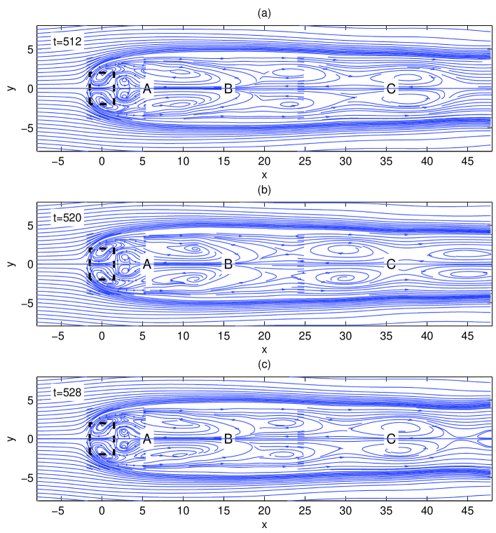
Figure 5: Instantaneous mass flow streamlines for the unperturbed symmetric inlet velocity profile: $t=$512($a$), 520($b$), 528($c$). $Re=900$, $N=9$. Dashed bold rectangle shows borders of the external magnet. Letters A at $x=5$, B at $x=15$, and $C$ at $x=35$ are points on the centerline, $y=0$, for time histories shown as dashed lines in Fig. 7.

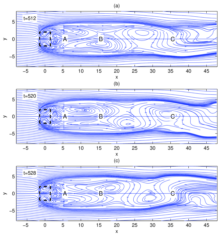
Figure 6: Instantaneous mass flow streamlines for the initially perturbed symmetric inlet velocity profile: $t=$512($a$), 520($b$), 528($c$). $Re=900$, $N=9$. Dashed bold rectangle shows borders of the external magnet. Letters A at $x=5$, B at $x=15$, and $C$ at $x=35$ are points on the centerline, $y=0$, for time histories shown as solid lines in Fig. 7.

Instantaneous mass flow streamlines for symmetric vortex shedding are shown in Fig. 5. They are plotted for the middle horizontal plane, $z=0$, and are symmetric with respect to the centerline $y=0$. There are three instances of time with $\Delta t=8$. For each, we see the same configuration of magnetic (first pair) and connecting (second pair) vortices, while attached vortices form a sequence dependent on the time instance. This provides evidence that the attached vortices come off the magnetic obstacle simultaneously and move downstream slowly. The location of the attached vortices in plot ($a$) ($t=512$) looks similar as in plot ($c$) ($t=528$), therefore one can conclude that vortex breakdown occurs at a time period equal to 16 time units.

Although symmetric vortex shedding past a bluff body is not typical in ordinary hydrodynamics, it is possible if one takes special steps, such as artificial forcing, see for instance Konstantinidis:Balabani:2007 , and references in Table 1 therein. The overwhelming majority of papers devoted to vortex shedding deals with an infinitely long cylinder. The MHD case under consideration is three-dimensional, i.e. there are top and bottom walls, so the proper hydrodynamic analogy is to consider a finite cylinder placed perpendicular between two endplates. There is evidence in ordinary hydrodynamics that the confinement imposed by the endplates increases the stability of the wake, see e.g. Shair:Grove:etal:1963 , Nishioka:Sato:1974 , Gerich:Eckelmann:1982 , Lee:Budwig:1991 . In particular, the range of the Reynolds number, $Re$, where two attached vortices remain symmetric behind a circular cylinder without breaking, is much larger in the presence of no-slip endplates. Therefore, it is also possible that the confinement stabilizes symmetric vortex shedding produced by the solid cylinder subject to the artificial forcing.

If the inlet velocity profile is not symmetric at initial times, then one expects an asymmetric vortex shedding, as shown in Fig. 6. The time instances are the same as in Fig. 5. One can see now that the attached vortices are shifted relative to each other through the centerline $y=0$. Plot $a$ ($t=512$) looks roughly like the mirror image of plot $c$ ($t=528$) giving by that evidence about the half-time period equal approximately to 16 time units. Altogether, the picture is similar to a standard time-periodic laminar vortex shedding past a solid circular cylinder. At the place of the cylinder there is a four-vortex ensemble composed of magnetic and connecting vortices. Because of Hartmann friction, this ensemble is stable in time, and so this represents the body of a virtual solid obstacle imposed by the external, strongly heterogeneous magnetic field.

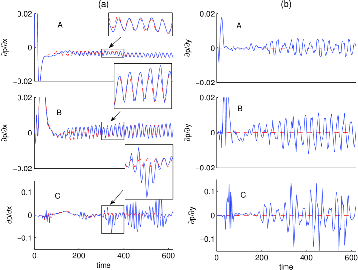
Figure 7: Streamwise ($\partial p/\partial x$, plot $a$) and crosswise ($\partial p/\partial y$, plot $b$) pressure gradients in points $A$, $B$, $C$ given in Fig. 5 (dashed) and 6 (solid lines). Insertions are zoomed for the time range $300\leq t\leq 400$.

Shown in Fig. 7 are time histories of local instantaneous streamwise ($\partial p/\partial x$, plot $a$) and crosswise ($\partial p/\partial y$, plot $b$) pressure gradients, for both symmetric (dashed) and asymmetric (solid lines) vortex shedding. The curves are given for points $A,B,C$ located on the centerline $y=0$ and denoted in Fig. 5 and Fig. 6. These pressure gradients are selected for time analysis because they can be measured experimentally. Moreover, $\partial p/\partial x$ and $\partial p/\partial y$ can be understood as the local drag and lift forces respectively. Time dependencies of drag and lift coefficients in the case of a solid cylinder are well understood, see e.g. Fig. 7 in Singh:Mittal:2005 . They are time-periodic with a single vortex shedding frequency at low Reynolds number.

As one can see in Fig. 7, the simulated $\partial p/\partial x$, $\partial p/\partial y$ first go through a transitional regime, which it is then transformed smoothly into a periodic regime. The time period, equal approximately to 16, can be estimated from the zoomed insertions plotted for the time range $300\leq t\leq 400$. (In these time dependent simulations the data were recorded every two time units, so the precision of the time period is plus/minus one.) It is easy to estimate roughly the Strouhal number $St=fL/u$. Here, $f=1/16$ is the frequency of vortex shedding, $L=2M_{y}=4$ is the crossstream size of the magnet, and $u=1$ is the mean flow velocity, so $St=1/4$. This value is different from that of 0.1 found in the paper by Cuevas et al. in 2D simulations. The difference is obviously explained by the impact of the channel walls. For the symmetric (dashed) and asymmetric (solid) vortex shedding, the streamwise pressure gradient has similar behavior at locations not far from the magnetic obstacle. One can see that $\partial p/\partial x$’s are very close at point $A$, slightly disagree at point $B$ and notably different at point $C$. The crosswise pressure gradient on the centerline for the symmetric shedding is equal to zero.

The generic scenario for the wake of the magnetic obstacle

In ordinary hydrodynamics, the generic scenario for the wake past the solid obstacle is the following when $Re$ smoothly increases Feynman:Lectures:Vol2:1964 before turbulence starts: (i) creeping flow, (ii) two attached vortices, (iii) vortex shedding. If one goes into the details, e.g. considers the different ways of vortex shedding, then different sub-scenarios can be found depending on specific conditions, but the generic character of the above classification remains. We emphasize that the interplay between the viscous and inertial forces is decisive for establishing this general peculiarities.

Analogously, by taking into consideration all possible forces, we derive now a scenario for the wake of the magnetic obstacle. This was given briefly before in Votyakov:PRL:2007 ; Votyakov:JFM:2007 without stressing that this is generic because of the lack at the time of information about vortex shedding. Now, this gap is filled.

In the case of the magnetic obstacle, there are three forces and three corresponding terms in the MHD equations: the viscous force (V), the inertial force (I), and the Lorentz force (L). If we put the forces in order of decreasing intensity, then the total number of all the possible relationships between forces is six: (1) VIL, (2) IVL, (3) VLI, (4) LVI, (5) LIV, and (6) ILV. (Each capital letter is given for the corresponding term.) The cases (1-2) are of the smallest Lorentz term, therefore, they can be treated as outlined above for the ordinary hydrodynamics. The cases (3-4) are of the smallest inertial term, therefore, there should be no attached vortices past the magnetic obstacle, so the possible scenario are either no vortices when the Lorentz force is smaller than the viscous force (case 3) or two alongside magnetic vortices when the Lorentz force is larger than the viscous force (case 4). Finally, the cases (5-6) are of the smallest viscous term and the peculiar patterns are either six vortices (case 5) when the inertial force is so low that the attached vortices are retained or vortex shedding with specific four-vortex pattern (case 6) as shown in previous Section. In the latter, the four vortices taken together is an analog of the bluff body as in the ordinary hydrodynamics.

It is important to stress that we discuss a 3D flow between two horizontal no-slip endplates. This discussion might be projected onto a 2D flow, but carefully. For instance, the 2D flow could not produce a 2D region excluded from the flow without violating the continuity requirement, $\nabla_{\perp}\mathbf{u}_{\perp}=0$. In a 3D flow, the latter equation is $\nabla\mathbf{u}=\nabla_{\perp}\mathbf{u}_{\perp}+\partial_{z}u_{z}=0$, which can be satisfied by the secondary flow in the third direction, i.e. by the $\partial_{z}u_{z}$ term. This results in the helical streamlines of magnetic vortices, see Fig. 11 in the paper by Votyakov et al. Votyakov:JFM:2007 . However, a 3D helix could not be realized in a 2D space, so the $u_{center}$, $E_{y,center}$ vanishing behavior shown in Fig. 3 becomes impossible. Instead, in the creeping 2D flow, $u_{center}$ is decreases as $N$ increases. Then, at some high critical $N$, a $u_{center}$ drop does stop and makes a flip into positive values causing two additional vortices in the core of the obstacle. This new resulting flow structure consists of four vortices as shown in Fig. 9$b$ of the paper by Cuevas et al. Cuevas:Smolentsev:Abdou:PRE:2006 . If $N$ increases further, then even more intricate recirculation patterns are produced. It looks paradoxical that a 3D flow has the simpler structure than a 2D flow, however, such simpler behavior is governed by a strong magnetic field, prohibiting a penetration into the core, and by the secondary flow in a vertical direction towards to Hartmann layers. Moreover, it is an issue how to practically realize a 2D creeping flow in order to reveal intricate recirculations in the 2D core without impact of top and bottom flow boundaries.

Another question that arises is whether the core of the magnetic obstacle appears for a sufficiently high $Re$ even at high $N$, that is, whether the upstream flow penetrates the stagnant core made of the magnetic and connecting vortices. Again, the answer depends on whether the flow considered is two- or three-dimensional. We suggest that the magnetic vortices must appear in both cases because $N$ is supposed to be sufficiently high to produce recirculation. So the question can be reformulated: whether the vortices and the stagnant core are stable.

In 2D simulations there is no sink for the upstream kinetic energy accumulated by the magnetic vortices. As a result, the rotating magnetic vortices are not fixed in their location and move freely in the plane by responding to the pulsations of the upstream flow. This destroys the core of the magnetic obstacle so it becomes penetrable. If there are small time-dependent pulsations in the upstream flow, then one can observe different (even exotic) configurations of magnetic vortices, which can be mistakenly taken as sub-scenarios of the given 2D simulation.

For any 2D approach applied to a realistic system, the main problem is whether 2D assumptions are reasonable because the realistic system has always endplates to hold magnetic poles. That is, the Hartmann friction and viscous friction are always present. Of course, to make 2D middle plane flow, the magnetic poles can be moved far apart while synchronously increasing the magnetic field intensity $B_{0}$ to keep the same $Ha$. But then, the gradient of the magnetic field becomes more smooth, therefore, one needs a higher critical $N_{c}$ to observe recirculation Votyakov:JFM:2007 .

In 3D simulations, there is a sink for the kinetic energy because the mass streamlines, that form magnetic vortices, represent helical trajectories into the Hartmann layers as shown recently in Votyakov:JFM:2007 . Then, the pulsations of the upstream kinetic energy are dissipated in the Hartmann layers by means of the friction with top/bottom walls. As a result, the rotating magnetic vortices are well fixed in their location and they do not move freely. Thus, when Hartmann layers are properly resolved in the 3D simulations and $N$ is enough high to induce alongside recirculation, then the core of the magnetic obstacle must be visible even at high $Re$.

To make more clear the aforesaid statement we consider the following two examples. First, one imagines a flow of moderate $Re_{1}$ and such a high $Ha_{1}$ that the core of the magnetic obstacle is stable. Then, by keeping $Ha_{1}$ constant, one increases $Re$, e.g. by taking a higher flow rate, to find $Re_{c}(Ha_{1})$ where the core destabilizes. This happens at a critical value $N_{c,1}=Ha_{1}^{2}/Re_{c}$. Now, one imagines a flow at moderate $Ha_{2}$ and such a high $Re_{2}$ that the core of the magnetic obstacle does not exist. Then, while keeping $Re_{2}$ constant, one increases $Ha$, e.g. by imposing a higher external magnetic field. There exists such a high $Ha_{c}(Re_{2})$ where the core stabilizes again. This happens at a critical value $N_{c,2}=Ha_{c}^{2}/Re_{2}$, which is supposed to be of the same order of magnitude as $N_{c,1}$. In other words, at any high constant $Ha$ it is possible to find $Re$ destabilizing the core, and vice verse, at any high constant $Re$, it is possible to find $Ha$ stabilizing the core.

Unfortunately, to confirm the above inference numerically is impossible because it requires expensive 3D simulations where the Hartmann layers must be properly resolved. For high $Re$ and $N$, the thickness of the Hartmann layers is $1/\sqrt{Re*N}$. Then, e.g. for $N=100$ (to guarantee magnetic vortices) and big $Re$ the grid resolution must be around $\delta/(10\sqrt{Re})$, where $1/\delta=3...10$ is the number of points to resolve Hartmann layers. If $Re=10000$, then around $(L_{y}/H)(L_{x}/H)10^{12}\sim 10^{15}$ numerical nodes is needed for every time step. The total number of time steps must be also very large to be sure that the magnetic vortices do not destroy the core of the magnetic obstacle. In the previous Section, $Re=900$ and $N=9$, and the core of the obstacle is shown to be stable.

Another interesting issue is whether the vortex shedding past the magnetic obstacle is similar to that past the solid obstacle. Indeed, the following is valid generally in both cases: (1) the attached vortices are formed from the creeping flow when $Re$ prevails a critical value; (2) in a certain range of $Re$, the attached vortices are stable; (3) when the inertial force exceeds the stable threshold, the attached vortices detach from the body. Because the inertial force is decisive in both cases and the Lorentz force vanishes past the magnetic obstacle, it is expected that the vortex shedding in both cases might be similar as well, at least for specially selected geometrical conditions. This issue is open currently.

Conclusion

In this paper, we attempted to shed light on the peculiarities of the MHD flow passing over a magnetic obstacle when the magnetic interaction parameter $N$ is large, i.e. strength of the magnetic field is high or when the Reynolds number $Re$, i.e. inertia of the flow, is large. The corresponding case for moderate $Re$ and $N$ has been elaborated in Votyakov:PRL:2007 ; Votyakov:JFM:2007 . As it turns out high values of $Re$ and $N$ neatly emphasize analogies between a magnetic and a solid obstacle that have been under discussion from the beginning of MHD in the former USSR. In this paper, we have illustrated, by means of 3D numerical simulations, how the core of the magnetic obstacle is formed when $N$ increases and examined the shedding of attached vortices when the $Re$ is high enough.

With regard to the core of the magnetic obstacle the open issue remains whether is possible to treat the problem in a simpler way based on the Kulikovskii’s approach Kulikovskii:1968 . This is an old and fruitful idea to subdivide the complicated MHD flow into two parts: core and periphery and then combine both parts with appropriate boundary conditions. It is shown in this paper that there must be three parts to include recirculation at high $N$: the rest of the flow, immovable core, and transitional region with magnetic vortices.

With regard to the shedding of vortices past a magnetic obstacle, it is confirmed that magnetic and connected vortices altogether represent a virtual bluff body, which is spatially fixed owing to the Hartmann friction Votyakov:PRL:2007 ; Votyakov:JFM:2007 . Because the virtual body is fixed, a stagnancy region is formed. In this region, the intensity of the magnetic field is negligible, hence, the Lorentz force vanishes and attached vortices are controlled only by the inertial force. The same happens past a solid obstacle. Then, it may appear that the regularities known for the attached vortices past a solid cylinder are valid also for those past a magnetic obstacle. This way of thinking is useful provided that one takes into consideration the three-dimensionality of the problem, namely, the fact that the cylinder is confined between two endplates.

References

- [1] P. Davidson. Magnetohydrodynamics in Materials Processing. Annual Review of Fluid Mechanics, 31:273–300, 1999.
- [2] A. Thess, E. V. Votyakov, and Y. Kolesnikov. Lorentz Force Velocimetry. Phys. Rev. Lett., 96:164501, 2006.
- [3] A. B. Tananaev. MHD duct flows. Atomizdat, Moscow, 1979.
- [4] R. Moreau. Magnetohydrodynamics. Kluwer Academic Publishers, Dordrecht, 1990.
- [5] P. A. Davidson. An introduction to Magnetohydrodynamics. Cambridge University Press, 2001.
- [6] U. Müller and L. Bühler. Magnetofluiddynamics in channels and containers. Springer, Berlin, 2001.
- [7] Y. M. Gelfgat, D. E. Peterson, and E. V. Shcherbinin. Velocity structure of flows in nonuniform constant magnetic fields 1. numerical calculations. Magnetohydrodynamics, 14:55–61, 1978.
- [8] Y. M. Gelfgat and S. V. Olshanskii. Velocity structure of flows in non-uniform constant magnetic fields. ii. experimental results. Magnetohydrodynamics, 14:151–154, 1978.
- [9] S. Cuevas, S. Smolentsev, and M. Abdou. Vorticity generation in creeping flow past a magnetic obstacle. Phys. Rev. E, 74:056301, 2006.
- [10] S. Cuevas, S. Smolentsev, and M. Abdou. On the flow past a magnetic obstacle. J. Fluid. Mech., 553:227 – 252, 2006.
- [11] S. Cuevas, S. Smolentsev, and M. Abdou. Vorticity generation in non-uniform mhd flows. In Proceedings of the Joint 15th Riga and 6th PAMIR International Conference. Fundamental and Applied MHD, volume 1, pages 25–32, Riga, Jurmala, Latvia, June 27-July 1, 2005.
- [12] E. V. Votyakov, Y. Kolesnikov, O. Andreev, E. Zienicke, and A. Thess. Structure of the wake of a magnetic obstacle. Phys. Rev. Lett., 98(14):144504, 2007.
- [13] E. V. Votyakov, E. Zienicke, and Y. Kolesnikov. Constrained flow around a magnetic obstacle. J. Fluid. Mech., 610:131–156, 2008.
- [14] J. A. Shercliff. The theory of electromagnetic flow-measurement. Cambridge University Press, 1962.
- [15] P. H. Roberts. An introduction to Magnetohydrodynamics. Longmans, Green, New York, 1967.
- [16] E. V. Votyakov, S. Kassinos, and X. Albets-Chico. Analytic models of heterogenous magnetic fields for liquid metal flow simulations. Theoretical and Computational Fluid Dynamics, in print, 2009.
- [17] E. Konstantinidis and S. Balabani. Symmetric vortex shedding in the near wake of a circular cylinder due to streamwise perturbations. Journal of Fluids and Structures, 23:1047–1063, October 2007.
- [18] E. V. Votyakov and E. Zienicke. Numerical study of liquid metal flow in a rectangular duct under the influence of a heterogenous magnetic field. Fluid Dynamics & Materials Processing, 3(2):97–113, 2007.
- [19] M. Griebel, T. Dornseifer, and T. Neunhoeffer. Numerische Strömungssimulation in der Strömungsmechanik. Vieweg Verlag, Braunschweig, 1995.
- [20] A.G. Kulikovskii. Slow steady flows of a conducting fluid at high hartmann numbers. Izv. Akad. Nauk. SSSR Mekh. Zhidk. i Gaza, (3):3–10, 1968.
- [21] Th. Alboussiere. A geostrophic-like model for large Hartmann number flows. J. Fluid. Mech., 521:125–154, 2004.
- [22] F. H. Shair, A. S. Grove, E. E. Petersen, and A. Acrivos. The effect of confining walls on the stability of the steady wake behind a circular cylinder. J. Fluid. Mech., 17:546–550, 1963.
- [23] M. Nishioka and H. Sato. Measurements of velocity distributions in the wake of a circular cylinder at low reynolds numbers. J. Fluid. Mech., 65:97–112, 1974.
- [24] D. Gerich and H. Eckelmann. Influence of end plates and free ends on the shedding frequency of circular cylinders. J. Fluid. Mech., 122:109–121, September 1982.
- [25] T. Lee and R. Budwig. A study of the effect of aspect ratio on vortex shedding behind circular cylinders. Physics of Fluids, 3:309–315, February 1991.
- [26] S. P Singh and S. Mittal. Flow past a cylinder: shear layer instability and drag crisis. International Journal for Numerical Methods in Fluids, 47:75–98, 2005.
- [27] Richard Feynman, Robert Leighton, and Matthew Sands. Lectures on physics. Vol II. Addison-Wesley, 1964.