A first orbital solution for the very massive 30 Dor main-sequence WN6h+O binary R145

Abstract

We report the results of a spectroscopic and polarimetric study of the massive, hydrogen-rich WN6h stars R144 (HD 38282 = BAT99-118 = Brey 89) and R145 (HDE 269928 = BAT99-119 = Brey 90) in the LMC. Both stars have been suspected to be binaries by previous studies (R144: Schnurr et al. 2008b; R145: Moffat 1989). We have combined radial-velocity (RV) data from these two studies with previously unpublished polarimetric data. For R145, we were able to establish, for the first time, an orbital period of 158.8 days, along with the full set of orbital parameters, including the inclination angle $i$, which was found to be $i=38^{\circ}\pm 9^{\circ}$. By applying a modified version of the shift-and-add method developed by Demers et al. (2002), we were able to isolate the spectral signature of the very faint-line companion star. With the RV amplitudes of both components in R145, we were thus able to estimate their absolute masses. We find minimum masses M${}_{\rm WR}sin^{3}i=(116\pm 33)$ M_⊙ and $M_{\rm O}sin^{3}i=(48\pm 20)$ M_⊙ for the WR and the O component, respectively. Thus, if the low inclination angle were correct, resulting absolute masses of the components would be at least 300 and 125 M_⊙, respectively. However, such high masses are not supported by brightness considerations when R145 is compared to systems with known, very high masses such as NGC3603-A1 or WR20a. An inclination angle close to 90^∘ would remedy the situation, but is excluded by the currently available data. More and better data are thus required to firmly establish the nature of this puzzling, yet potentially very massive and important system. As to R144, however, the combined data sets are not sufficient to find any periodicity.

1 Introduction

Fundamental questions of stellar astrophysics suffer from a lack of truly empirical evidence when it comes to stars with the highest masses both on and evolved off the main sequence (MS). Recent models maintain that in the early Universe, the initial-mass function (IMF) was top-heavy and that primordial (Population III) stars were extremely massive, with masses from $\sim$100 to $\sim$1000 M_☉ (Ostriker & Gnedin 1996; Nakamura & Umemura 2001; Schaerer 2002). In contrast to that, recent studies have put forward both theoretical and observational arguments that under present-day conditions, an IMF cut-off occurs around $\sim 150$ M_☉ (Weidner & Kroupa 2004; Figer 2005). However, even in the Local Group very massive stars remain poorly characterized, and it so far remains uncertain at what mass an upper cut-off really occurs, if at all.

The least model-dependent and thus most reliable way to directly measure stellar masses is by Keplerian orbits in binary systems. In the past years, studies of very massive binaries have yielded the somewhat surprising results that the most massive stars known are to be found not among O-type stars, but among a very luminous subtype of Wolf-Rayet (WR) stars, the so-called WN5-7h (or ha) stars. These hydrogen-rich WN stars are young, unevolved objects rather than “classical” WR stars, which are usually identified with evolved, helium-burning, massive stars (de Koter et al. 1997; Crowther & Dessart 1998). WN5-7h stars mimic classical, i.e. evolved, core helium burning WR stars because their extreme luminosity, a result of their very high masses, drives a dense and fast wind which gives rise to WR-like emission lines. Due to the rarity of very massive stars in general and of very massive binaries in particular, only few massive systems have been “weighed” so far. In order of increasing mass, these are the Galactic Wolf-Rayet stars WR22 (72 M_☉ for the WN7h component (Rauw et al., 1996), although Schweickhardt et al. (1999) derive only 55 M_☉), WR20a (83 and 82 M_☉ for both WN6ha components; Rauw et al. 2004; Bonanos et al. 2004), WR21a (minimum mass $M\sin^{3}i=87$ M_☉ for the O3If/WN6 primary; (Niemela et al., 2008)), NGC3603-A1 (116 and 89 M_☉ for both WN6ha components; Schnurr et al. 2008a). Clearly, these very high masses impressively underline the extraordinary nature of WN5-7h stars.

In a recent, intense survey of 41 of the 47 known WNL stars in the LMC, Schnurr et al. (2008b, hereafter S08) used 2m-class telescopes to obtain repeated, intermediate-quality (R=1000, S/N$\sim$80) spectra in order to assess the binary status of the 41 targets from radial-velocity (RV) variations. S08 identified four new binaries containing WN5-7h stars, bringing the total number of known WNLh binaries in the LMC to nine. For one of the previously known binaries, R145 (= HDE 269928 = BAT99-119 = Brey 90), the preliminary 25.4-day period reported by Moffat (1989, hereafter M89) could not be confirmed, but neither could a coherent period be established from the RV data of this study alone. Therefore, we combined S08’s RVs with those published by M89, and with previously unpublished polarimetry. It was only after the combination that we were able to find the true orbital period of this system as well as other orbital parameters.

From both its RV and EW variations and its high X-ray luminosity, S08 identified another WN6h star, R144 (HD 38282 = BAT99-118 = Brey 89), to be a binary candidate, although M89 had identified this star as probably single. In terms of spectral type, R144 is almost a perfect clone of R145; however, at the $\sim$same bolometric correction and after allowing for differential interstellar extinction, R144 is $\sim$0.5 mag brighter than R145. Indeed, Crowther & Dessart (1998), using atmosphere models without iron-line blanketing, derived a spectroscopic mass in excess of 100 M_☉, and a luminosity of log$L/L_{\sun}=6.34$ for R144, which makes this star one of the most luminous WR stars known. New, updated models most likely would yield an even higher mass and luminosity, making R144 the most luminous main-sequence (MS) object in the Local Group. Since we also have unpublished polarimetry for R144, we have revisited this object as well, using the spectroscopic data obtained by S08.

In the present paper, we will report the results of this study. In Section 2, we will briefly describe the observations and the data reduction. In Section 3, we will describe the analysis of our data and present the results. The paper is then summarized in Section 4.

2 Observations and Data Reduction

2.1 Spectroscopy

The spectroscopic observations are described in detail in S08. We briefly recapitulate here that long-slit spectrographs attached to ground-based, southern, 2m-class telescopes were used. Data were obtained in three observing seasons between 2001 and 2003 to maximize the time coverage, and were carried out during 13 runs at 6 different telescopes. The spectral coverage varied from one instrument to another, but all spectrographs covered the region from 4000 to 5000 Å, thereby encompassing the strategic emission line He ii $\lambda$4686

Data were reduced in the standard manner using NOAO-IRAF, and corrected for systematic shifts among different observatories (see S08 for more details). The achieved linear dispersion varied from 0.65 Å/pixel to 1.64 Å/pixel, but all data were uniformly rebinned to 1.65 Å/pixel, thereby yielding a conservative 3-pixel resolving power of $R\sim 1000$. The achieved signal-to-noise (S/N) ratio was $\sim$ 120 per resolution element for both stars, as measured in the continuum region between 5050 and 5350 Å.

Additional RV data for R144 and R145 were taken from M89, to which we refer for more details on the data acquisition and reduction.

2.2 Polarimetry

Linear polarimetry in white light was obtained during a total of six observing runs between October 1988 and May 1990 at the 2.2m telescope of the Complejo Astronómico El Leoncito (CASLEO) near San Juan, Argentina, with VATPOL (Magalhaes et al. 1984), and at the ESO/MPG-2.2m telescope at La Silla, Chile, with PISCO (Stahl et al. 1986). RCA GaAs phototubes were employed in both cases. Exposure times were typically 15 minutes per data point. Appropriate standard stars were taken to calibrate the polarization angle and the zero level, and exposures of the adjacent sky were obtained to correct for the background count rates.

The polarimetric data were calibrated the usual way (e.g. Villar-Sbaffi et al. 2006). Since Thompson scattering is wavelength-independent (i.e. grey), and the differences between the sensitivity curves of the respective detectors are small, no correction for the different passbands was deemed necessary. However, a small instrumental offset between PISCO and VATPOL was found in polarization; we therefore have added $\Delta Q=0.10\%$ and $\Delta U=0.10\%$ to the PISCO data to match the VATPOL data, on average. The final polarimetric data for R144 and R145 are listed in Tables 1 and 2, respectively.

Statistics reveal that R144 displays a small but significant scatter (standard deviation) about their mean values in both Stokes parameters, 0.052% and 0.063% in $Q$ and $U$, respectively; by comparison, the quoted error per data point is only $\sim$half this. However, in Figure 1 one can clearly see that over the observation period of $\sim$15 days, the polarization in Stokes-$U$ increases constantly by $\sim$0.2% (i.e. $\sim$seven times the quoted error per data point), while Stokes-$Q$ also shows systematic variability, which is a strong indication that some coherent process is involved, e.g. a (longer-period) binary motion.

R145, on the other hand, is much more variable; the scatter is 0.26% and 0.20% about their mean values, respectively, in $Q$ and $U$, with well defined and coherent variability episodes (Figure 2).

Table 1: Linear polarimetry for R144, obtained with VATPOL at CASLEO over a two-week period in January 1990.

HJD	$Q$	$\sigma_{Q}$	$U$	$\sigma_{U}$	Instrument
2447907.783	-0.292	0.022	0.175	0.022	VATPOL
2447908.819	-0.213	0.031	0.112	0.031	VATPOL
2447909.813	-0.103	0.028	0.099	0.028	VATPOL
2447910.681	-0.136	0.020	0.206	0.020	VATPOL
2447911.754	-0.131	0.026	0.204	0.026	VATPOL
2447912.754	-0.084	0.025	0.160	0.025	VATPOL
2447913.566	-0.162	0.020	0.188	0.020	VATPOL
2447914.628	-0.134	0.035	0.213	0.035	VATPOL
2447915.762	-0.138	0.021	0.220	0.021	VATPOL
2447916.758	-0.103	0.028	0.232	0.028	VATPOL
2447917.803	-0.194	0.030	0.218	0.030	VATPOL
2447919.763	-0.179	0.031	0.308	0.031	VATPOL
2447920.753	-0.173	0.025	0.277	0.025	VATPOL
2447921.699	-0.180	0.025	0.279	0.025	VATPOL
2447923.789	-0.170	0.025	0.310	0.025	VATPOL

Table 2: Linear polarimetry for R145, obtained with PISCO at ESO and VATPOL at CASLEO, between October 1988 and May 1990.

HJD	$Q$	$\sigma_{Q}$	$U$	$\sigma_{U}$	Instrument
2447438.872	-2.244	0.028	0.552	0.028	PISCO
2447440.856	-1.746	0.020	0.551	0.020	PISCO
2447442.832	-1.517	0.020	0.447	0.020	PISCO
2447444.810	-1.386	0.022	0.811	0.022	PISCO
2447446.838	-1.718	0.024	1.119	0.024	PISCO
2447449.858	-2.626	0.027	0.822	0.027	PISCO
2447449.839	-2.542	0.025	0.573	0.025	PISCO
2447451.853	-2.029	0.024	0.457	0.024	PISCO
2447452.852	-1.771	0.025	0.408	0.025	PISCO
2447437.859	-2.048	0.032	0.473	0.032	VATPOL
2447438.849	-1.969	0.029	0.476	0.029	VATPOL
2447439.843	-1.926	0.027	0.502	0.027	VATPOL
2447440.856	-1.835	0.019	0.451	0.019	VATPOL
2447441.854	-1.839	0.027	0.472	0.027	VATPOL
2447442.873	-1.502	0.038	0.589	0.038	VATPOL
2447444.848	-1.586	0.023	0.843	0.023	VATPOL
2447445.858	-1.748	0.027	1.009	0.027	VATPOL
2447472.852	-2.202	0.029	0.388	0.029	VATPOL
2447473.810	-2.105	0.021	0.800	0.021	VATPOL
2447476.819	-2.198	0.021	0.714	0.021	VATPOL
2447477.812	-2.181	0.021	0.642	0.021	VATPOL
2447478.815	-2.211	0.023	0.676	0.023	VATPOL
2447479.803	-2.182	0.018	0.701	0.018	VATPOL
2447480.824	-2.162	0.020	0.736	0.020	VATPOL
2447481.819	-2.238	0.021	0.736	0.021	VATPOL
2447482.772	-2.131	0.019	0.693	0.019	VATPOL
2447860.775	-2.259	0.016	0.614	0.016	VATPOL
2447861.785	-2.236	0.017	0.591	0.017	VATPOL
2447862.779	-2.155	0.020	0.618	0.021	VATPOL
2447863.807	-2.258	0.019	0.682	0.019	VATPOL
2447864.793	-2.183	0.017	0.626	0.017	VATPOL
2447865.715	-2.218	0.018	0.569	0.018	VATPOL
2447866.733	-2.157	0.014	0.635	0.014	VATPOL
2447907.768	-2.301	0.019	0.567	0.019	VATPOL
2447908.808	-2.356	0.033	0.309	0.033	VATPOL
2447909.802	-2.261	0.029	0.150	0.029	VATPOL
2447910.671	-2.236	0.027	0.186	0.027	VATPOL
2447911.745	-2.061	0.029	0.329	0.029	VATPOL
2447912.742	-2.124	0.029	0.462	0.029	VATPOL
2447913.379	-2.024	0.025	0.430	0.025	VATPOL
2447915.774	-2.038	0.031	0.418	0.031	VATPOL
2447916.772	-1.884	0.021	0.496	0.021	VATPOL
2447917.792	-1.877	0.029	0.417	0.029	VATPOL
2447918.713	-1.921	0.025	0.518	0.025	VATPOL
2447919.751	-1.716	0.028	0.550	0.028	VATPOL
2447920.739	-1.732	0.027	0.644	0.027	VATPOL
2447921.690	-1.692	0.025	0.912	0.025	VATPOL
2447922.733	-1.849	0.027	1.040	0.027	VATPOL
2447923.772	-2.216	0.027	1.090	0.027	VATPOL
2447974.536	-2.186	0.024	0.719	0.024	VATPOL
2447975.531	-2.229	0.028	0.654	0.028	VATPOL
2447976.579	-2.239	0.032	0.648	0.032	VATPOL
2447977.559	-2.244	0.030	0.607	0.030	VATPOL

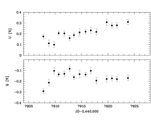
Figure 1: Polarimetric data for R144 plotted versus Julian date.

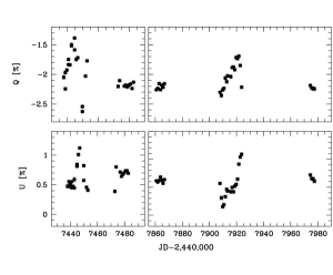
Figure 2: Polarimetric data for R145 plotted versus Julian date. Note the enormous amplitude of $\sim$1%, rarely seen so large in other WR+O systems.

3 Data Analysis and Results

3.1 Spectroscopic Data

We here only briefly describe the methods employed to extract radial velocities (RVs) from the spectra (for details we refer the reader to S08 and references therein): Cross-correlation and emission-line fitting routines programmed using the ESO-MIDAS tasks XCORR/IMA and FIT/IMA, respectively, with an iterative approach for cross-correlation.

Since the spectra of both R144 and R145 are largely dominated by the strong He ii $\lambda$4686 emission line (see Figure 3), we initially confined cross-correlation to this line to derive RVs for R145, but then applied the method to the He ii $\lambda$5412 line as well. Furthermore, RVs from the faint, but very narrow N iv $\lambda$4058 emission were obtained by fitting Gauss profiles to the line.

Unfortunately, due to low S/N and an unreliable wavelength calibration at the blue end of our spectra (the comparison-arc lamp has practically no useful lines in this region; see S08 for more details), the N iv $\lambda$4058 line yielded much worse RV scatter than the two He ii lines. Thus, the main part of the analysis was carried out with the two, much stronger He ii lines

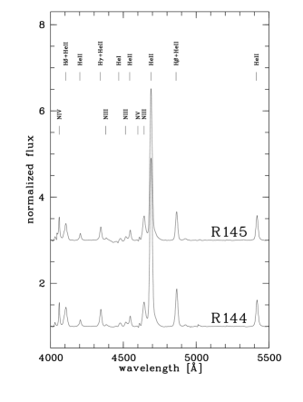
Figure 3: Mean spectra of R144 and R145. For clarity, the upper spectrum has been shifted by 2 flux units.

Fitting a Gauss function to the He ii $\lambda$4686 emission yielded a slightly larger scatter than cross-correlation, but was used to measure absolute, systemic velocities. These absolute velocities were then used to correct the relative RVs obtained by cross-correlation, and to combine our data with those of M89. Initially, a possible zero-point shift between S08 and M89 was not corrected for (but see below). Unfortunately, M89’s spectra did not cover He ii$\lambda$5412, so that only RV data from He ii $\lambda$4686 and N iv $\lambda$4058 could be combined. The combined RV data for He ii $\lambda$4686 are shown in Figure 4.

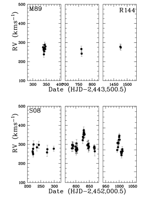
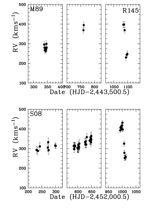
Figure 4: RV data obtained from He ii $\lambda$4686 of R144 (left) and R145 (right). Shown are the three observing seasons of M89 (upper panels) and S08 (lower panels), respectively.

3.2 Search for Periodicities in the RV Curves

As reported by S08, a comprehensive period analysis using different methods of their RV data in the range from 1 to 200 days yielded no coherent period for R145. We repeated this analysis on the combined S08+M89 data set, also without success. Additionally, we tried to apply the phase-dispersion minimization (PDM) method (Stellingwerf 1978), which is very reliable because it does not assume a specific wave form (e.g. sinusoids) and which is therefore very useful for strongly eccentric binaries with highly distorted RV curves. Unfortunately however, the data are too dispersed for periods much longer than 100 days, so the PDM suffers from many severely depleted or downright empty phase bins. Thus, a different approach was used.

3.2.1 R144

On close inspection in Figure 4, R144 does not show any clearly repeating pattern in S08’s RV data, which is the reason why S08 were not able to establish a period in the first place, and there certainly is no pattern at all visible in the M89 data set. We therefore have to conclude that better data are required for R144, if any periodicity is to be found. Long-term monitoring is being undertaken.

3.2.2 R145

Inspection of R145’s RV curves in Figure 4 reveals a repeating pattern: In both M89’s and S08’s last observing season, the RV curve drops from its highest to its lowest value within a very short interval of time. This event can consistently be interpreted as the periastron passage (PP) of a highly eccentric, long-period binary. But what is its period? We are lucky, because it seems that we have three such PP events recorded: two in the M89 data set (called PP1 and PP2), and one in the S08 data set (PP3). We further distinguish the highest and the lowest RVs during the respective event; thus, we find that the combined RV data set covers the following events: PP1 high, PP2 high and low, PP3 high and low. Julian Dates and RVs for each event are given in Table 3.

Table 3: Measured dates and RVs for the presumed periastron-passage (PP) events PP1 through PP3 in the data sets of M89 and S08, respectively. “High” and “low” refer to maximum and minimum RVs measured just before and after the supposed PP, respectively. See text for more details.

Data set	Event	MJDa	RVb
			[kms-1]
M89	PP1 high	44261.4	423 $\pm 15$
M89	PP2 high	44584.4	424 $\pm 15$
M89	PP2 low	44599.5	276 $\pm 15$
S08	PP3 high	53001.8	432 $\pm 15$
S08	PP3 low	53012.4	252 $\pm 15$
aJD-2,400,000.5
berrors are estimated

It seems that the duration of the PP2 event is somewhat longer than that of the PP3 event, $\sim$15 versus $\sim$10 days. However, the observed RV amplitude during PP2 is smaller than that observed during PP3. It is thus likely that the true minimum RV was missed during the observations of the PP2 “low” event, thus the full RV peak-to-valley swing of the WR star (i.e., $2K$) might be closer to the value obtained from PP3, $\Delta RV(PP3)=180$ kms^-1.

Measuring the elapsed time between corresponding events yields the following time intervals, each of which will be an integer multiple of the period, assumed, of course, there is one:

$$\Delta T_{\rm 31,hi}=MJD(\rm PP3_{hi}-PP1_{hi})=(8740.4\pm 6)days$$

$$\Delta T_{\rm 32,hi}=MJD(\rm PP3_{hi}-PP2_{hi})=(8417.4\pm 6)days$$

$$\Delta T_{\rm 32,lo}=MJD(\rm PP3_{lo}-PP2_{lo})=(8412.9\pm 6)days$$

$$\Delta T_{\rm 21,hi}=MJD(\rm PP2_{hi}-PP1_{hi})=(323.0\pm 6)days,$$

where the overall, quadratic error has been obtained from $\sqrt{4^{2}+4^{2}}\sim 6$. From $\Delta T_{21,hi}$ follows that the longest possible period is $(323\pm 6)$ days; otherwise, two high events would occur during one orbit. The true period is thus an integer fraction of this period, i.e. $(323\pm 6)/n$ days, with $n=1..5$, since any period shorter than $\sim$60 days is ruled out by S08’s observations; it follows that there are five groups of periods, $323\pm 6$, $161.5\pm 3$, $107.67\pm 2$, $80.75\pm 1.5$, and $64.6\pm 1.2$ days. Within each group, the longer time intervals are used to refine the results and to obtain more precise periods. Periods which, within their errors, are consistent with each other, are averaged, and a quadratic mean error is computed. The resulting periods are listed in Table 4.

Table 4: The five groups of possible orbital periods of R145 as computed from the condition that the true period has to be an integer fraction $n$ of the respective time interval $\Delta T_{\rm 21,hi}$, $\Delta T_{\rm 32,lo}$, $\Delta T_{\rm 32,hi}$, and $\Delta T_{\rm 31,hi}$. For each group, the typical error on the period is given. Periods that are consistent with each other within these errors, have been averaged to yield $P_{\rm mean}$ and the mean error.

Possible periods (in days)
$P_{\rm 21,hi}$	$P_{\rm 32,lo}$	$P_{\rm 32,hi}$	$P_{\rm 31,hi}$	$P_{\rm mean}$
323.00	323.573	323.746	323.719	323.679
$\pm$6.00	$\pm$0.231	$\pm$0.231	$\pm$0.222	$\pm$0.228
161.50	161.787	161.874	161.859	161.840
$\pm$3.00	158.734	158.819	158.916	158.823
	$\pm$0.115	$\pm$0.115	$\pm$0.111	$\pm$0.114
107.67	106.492	106.549	106.590	106.544
$\pm$2.00	107.858	107.915	107.906	107.906
	109.258	109.317	109.255	109.277
	$\pm$0.078	$\pm$0.078	$\pm$0.075	$\pm$0.077
80.75	79.367	79.409	79.458	79.411
$\pm$1.50	80.123	80.166	80.187	80.159
	80.893	80.937	80.930	80.902
	81.679	81.722	81.686	81.696
	$\pm$0.058	$\pm$0.058	$\pm$0.056	$\pm$0.057
64.60	63.734	63.763	63.799	63.765
$\pm$1.20	64.221	64.255	64.268	64.248
	64.715	64.749	64.744	64.736
	65.216	65.251	65.227	65.231
	65.726	65.761	65.717	65.735
	$\pm$0.047	$\pm$0.047	$\pm$0.043	$\pm$0.046

Since the data are too sparse, an automated phase-dispersion minimum method (Stellingwerf 1978) is not possible; we thus folded the data into the respective phases and chose the most coherent-looking curve by eye. This method is of course limited; for instance, there are no noticeable differences in the RV curves of the 323-day and 161.5-day periods within a given group. Hence, the selected RV curves shown in Figure 5 are representative. However, the groups of periods around 107.67, 80.75, and 64.60 days can readily be ruled out as they yield incoherent RV curves.

The longest possible (and unique) period, $323.679$ days, results in a very well-defined RV curve and a very eccentric orbit; however, it does so by construction and, more importantly, shows a data gap of almost exactly half a phase, which is suspicious. The periods around $161.5$ days also yield coherent RV curves, but with a much better phase coverage, and a slightly less eccentric orbit, as can already be seen by eye.

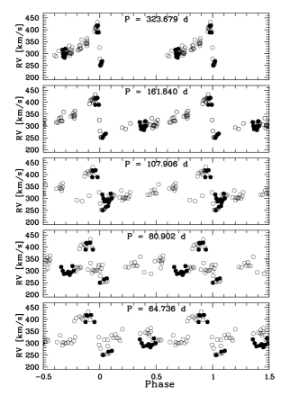
Figure 5: Combined RV data of R145 obtained from He ii $\lambda$4686 (M89: filled; S08: empty symbols) and folded into the corresponding phases of five different, possible periods based on $P_{\rm mean}$ in Table 4.

3.3 Polarimetric Data

With these results from the spectroscopy, we proceeded to analyze the polarimetric data. To derive the orbital parameters, we used the elliptical orbit model by Brown et al. (1982) with the correction by Simmons & Boyle (1984), modified for an extended source of scatterers (cf. Robert et al. 1992), i.e. assuming an ensemble of optically thin, free electrons that follow the wind density around one of the stars spherically symmetrically (for details, see Moffat et al. 1998).

For R144, the fit did not converge, and since there is no orbital solution from the spectroscopy, we were unable to constrain the fit. This does not entirely come as a surprise, given the small number of data points ($N=15$) spread over only $\sim$2 weeks, and the rather small level of variability. Thus, we abandon the study of R144 based on the current data.

For R145, however, the fit of the polarization data alone yielded a coherent solution with a period of $P=(159\pm 1)$ days, which is consistent with the lower boundary of $P_{\rm 21,hi}$ (see above), but has consequences that will be discussed below. Encouraged by this result, we combined the spectroscopic (i.e., M89+S08) and polarimetric data sets, and forced a simultaneous fit. For cross-verification, we also used the RV data that were obtained from the slightly weaker, but less perturbed, He ii $\lambda$5411 emission line, with similar results.

Note that the fits to the respective data sets do not have all orbital parameters in common. For instance, spectroscopy cannot yield the inclination angle $i$ and the orientation of the line of nodes $\Omega$, both of which are calculated from the polarimetry. Thus, only the following parameters were obtained from the fit of the combined RV and polarimetric data: Interstellar polarization $Q_{0}$ and $U_{0}$; $\Omega$ (see above); the orbital inclination angle $i$; the orbital longitude of the centroid of the scattering region at periastron passage $\lambda_{p}$ (linked to the argument of the periastron by the relation $\lambda_{p}=\omega-90^{\circ}$); the orbital period $P$; the RV amplitude $K_{\rm WR}$ of the WR component; the systemic velocity $V_{0}$; the systematic RV shift between the M89 and S08 data sets $\Delta V$; the orbital eccentricity $e$; the time of periastron passage $T_{0}$; the total electron scattering optical depth $\tau$ (assuming Thompson scattering to be the only source of opacity); the exponent $\gamma$ in the power law describing how the electron density falls off from the WR stars (e.g., $\gamma=2$ for an inverse square law around a scattering point source); the possible systematic shift between the two RV data sets $\Delta RV=\rm S08-M89$.

In order to facilitate convergence, the fit was carried out for three parameter groups which are, to first order, independent of each other: 1. ($K$, $V_{0}$, $\Delta RV$); 2. ($Q_{0}$, $U_{0}$, $\tau$, $\gamma$); 3. ($i$, $\Omega$, $\lambda_{p}$, $e$). One group was fitted while the two others were kept constant. For each permutation $\chi^{2}$ was computed, and the procedure was repeated until the fit yielded a constant $\chi^{2}$ for all permutations. In order to estimate the errors on individual fit parameters, we explored the sensitivity of the fit (i.e., its $\chi^{2}$) by varying one parameter around its best-fit value (obtained from the overall fit) while keeping all other parameters constant. Those variations of each individual parameter which resulted in a 5% deterioration of the $\chi^{2}$ compared to its minimum value from the overall fit, were used as error levels of the respective parameter. Results of the fits for both He ii $\lambda$4686 and He ii $\lambda$5411 are shown in Table 5. The resulting orbital solutions together with the polarimetric data folded into the corresponding phase is shown in Figure 6.

Table 5: Orbital parameters from the combined fit of both the spectroscopic and the polarimetric data sets.

Parameter	He ii $\lambda$4686			He ii $\lambda$5411
$\tau$ [%]	0.048	$\pm$	0.006	0.049	$\pm$	0.006
$Q_{0}$ [%]	-2.17	$\pm$	0.04	-2.18	$\pm$	0.04
$U_{0}$ [%]	0.67	$\pm$	0.04	0.68	$\pm$	0.04
$\Omega$ [∘]	-40	$\pm$	7	-42	$\pm$	7
$i$ [∘]	37	$\pm$	7	39	$\pm$	6
$\omega$ = $\lambda_{p}+90[^{\circ}]$	85.0	$\pm$	6.7	83.4	$\pm$	6.6
$P$ [days]	158.8	$\pm$	0.1	158.8	$\pm$	0.1
$K_{\rm WR}$ [kms-1]	81	$\pm$	21	93	$\pm$	21
$\Delta RV^{a}$ [kms-1]	10	$\pm$	29		n/a
$e$	0.70	$\pm$	0.02	0.69	$\pm$	0.02
$V_{0}$ [kms-1]	328	$\pm$	14	382	$\pm$	13
$T_{0}$ [JD-2,450,000.5]	3007.763	$\pm$	0.25	3007.763	$\pm$	0.25
$\gamma$	1.70	$\pm$	0.15	1.75	$\pm$	0.14
${}^{a}\Delta RV$=S08-M89

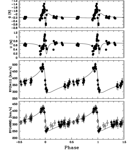
Figure 6: Orbital solution for R145 obtained from the simultaneous fit of the the Stokes $Q$ and $U$, and RV data sets. For the He ii $\lambda$4686 emission line (bottom panel), S08 data are shown in filled symbols, and M89 data are shown in empty symbols. The systematic shift between the two RV data sets, $\Delta RV$, has been applied. For He ii $\lambda$5411, only S08 data could be used for the fit, which is why there are fewer data points.

The difference in the systemic velocities obtained from He ii $\lambda$4686 and $\lambda$5411 amounts to $\sim$55 kms^-1. It is well known in the literature that systemic velocities obtained from emission lines of WR stars display a systematic red-shift with respect to the true systemic velocity (e.g. of the host galaxy of the WR star, see e.g. S08). This phenomenon can be explained by radiative-transfer effects (cf. Hillier 1989). However, it is noteworthy that different lines of the same ionic species will display significantly different systemic velocities. Cross-verification with R144 yielded the very same effect with roughly the same shift ($\sim$50 kms^-1) between the systemic velocities obtained from the two He ii lines, and shows that the effect is indeed real.

However, in WR+O binaries, He ii emission lines are prone to suffer from profile variations due to excess emission arising in the wind-wind collision (WWC) region; therefore they might not yield the correct, but a more or less distorted RV curve (and with this, wrong orbital parameters). Indeed R145 displays strong excess emissions, and because R145 is a very eccentric system, the strength of the excess emission varies considerably over the orbital phase. From simple considerations, we expect (and find; see Section 3.6 for a more detailed discussion) the excess emission to be strongest near periastron. This, however, means that the RVs derived from line profiles of both He ii $\lambda$4686 and $\lambda$5411 are most affected at an orbital phase where the RV data points have the most importance for the orbital fit, namely when the RV of the WN component changes quickly from maximum redshifted to maximum blueshifted velocities, around periastron passage.

To somewhat reduce the effect of such line-profile variations over the orbital cycle, we have employed the iterative cross-correlation method described in S08. In fact, Foellmi et al. (2003) have shown that using bisectors to measure the line center yields perfectly similar results to those obtained by iterative cross-correlation (with bisectors yielding a slightly larger scatter). Thus, the iterative form of cross-correlation is relatively robust against the influence even of strong and variable WWC excess emissions.

Furthermore, we have investigated how the emission-line strength changes over the orbital cycle due to the variable strength of the excess emissions. We measured the equivalent widths (EWs) of both He ii $\lambda$4686 and $\lambda$5411, normalized them by the mean value around apastron (phase interval [0.4;0.6]) when the WWC excess emissions supposedly are weakest, and folded these relative EWs into the orbital phase (for $P=158.8$ days; see Figure 7). Despite the fact that He ii $\lambda$4686 suffers more from the increased WWC excess emission at periastron (almost twice compared to He ii $\lambda$5411), the orbital solutions the respective lines are fully consistent with each other, the only difference being the redshifted systemic velocity of He ii $\lambda$5411, as discussed above.

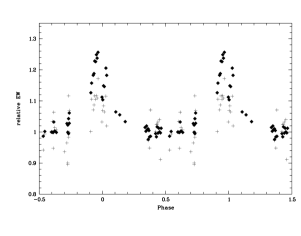
Figure 7: Relative EWs (normalized to unity around apastron, i.e. $\phi=0.5$) of the two emission lines He ii $\lambda$4686 (filled lozenges) and $\lambda$5411 (crosses). While He ii $\lambda$5411 yields more noise because it is the weaker line, He ii $\lambda$4686 suffers from almost twice the line-strength variability due to increased WWC excess emission around periastron (i.e. $\phi=0$). Yet both lines yield consistent orbital parameters.

As an additional test, we have used RVs obtained from Gauss-fitting the weak and narrow, highly-ionized N iv $\lambda$4058 emission line. As before, our results were combined with those published by M89 using the systematic shift between the two data sets obtained from the orbital fitting of He ii $\lambda$4686 ($\Delta RV$ of 10 kms^-1; see Table 5). Due to its fluorescent origin from ultra-violet transitions (cf. Hillier 1988), the N iv $\lambda$4058 line is commonly regarded as very robust against WWC excess emissions, and usually yields RVs which follow best the true orbital motion of the WR star. In Figure 8 we have plotted the orbital solution obtained from He ii $\lambda$4686. Overplotted are the combined RVs obtained from N iv $\lambda$4058, shifted by +110 kms^-1 to match the mean velocity of the orbital solution. While the scatter of the data points is expectedly large (see Section 3.1), which makes it impossible to use this line for a sensible orbital fit, the points do follow the orbital motion and, more importantly, do not show a significantly different RV amplitude. Even if this is not fully conclusive evidence, it is a very plausible indicator that the orbital parameters obtained from the RVs of the two He ii lines are reliable. Moreover, since the orbital solutions were obtained from a combined set of spectroscopic and polarimetric data, and the latter is not affected by line-profile variations, the influence of WWC excess emission is further attenuated.

Since N iv $\lambda$4058 does not suffers from radiative-transfer effects like the He ii lines, and is not blended, it also yields a relatively precise estimate of the true systemic velocity of the WR star; Moffat & Seggewiss (1979) found a small, negative shift for Galactic WN7/WN8 stars, $(-15\pm 13)$ kms^-1 (standard deviation). Using the mean velocity of the N iv $\lambda$4058 line as an estimate of the true systemic velocity of the binary system, we thus obtain $\overline{RV}(4058)=(220\pm 30)$ kms^-1. This value is just inconsistent with the reported systemic velocity of the LMC, $v_{\rm sys}=(280\pm 20)$ kms^-1 (Kim et al. 1998). Either for some reason, N iv $\lambda$4058 has a rather exceptional negative RV, or R145 indeed has a slightly negative systemic velocity with respect to the LMC.

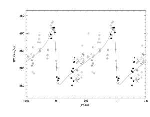
Figure 8: Orbital solution as obtained from the He ii $\lambda$4686 emission line (solid line) and RVs obtained from N iv $\lambda$4058 (lozenges; filled symbols are from M89, empty symbols are based on the S08 data). While the scatter of the RVs obtained from the N iv $\lambda$4058 emission is very large, there is no indication that the motion of He ii $\lambda$4686 is systematically different.

Based on our error-estimation method, the error for the inclination angle $i$ was found to be 7^∘ and 6^∘ for the two lines He ii $\lambda$4686 and $\lambda$5411, respectively. Choosing a higher cut-off value than the 5% used will of course lead to a larger error on $i$ (and all other parameters), but the $\chi^{2}$ deteriorates very quickly when the inclination angle varies by much more than 10 to 15^∘, and the discrepancies between the fit and the data become noticeably large. However, it is well known among polarimetrists that, due to an asymmetric error distribution, there is a bias of the polarimetric determination of the inclination angle towards higher values than the true value of $i$; this bias is more pronounced, the lower the true inclination angle and the lower the data quality is (in terms of both the number of available data points and their respective individual errors); see e.g. Aspin et al. (1981), Simmons et al. (1982) or, more recently, Wolinski & Dolan (1994) for a comprehensive discussion of this issue. Thus, our analysis is bound to overestimate the true value of $i$, which means that the true inclination angle is more likely lower than $39^{\circ}$, rendering the resulting masses even higher and less plausible (see below). If, on the other hand, we were to force a fit with the inclination angle fixed at $90^{\circ}$, the resulting $\chi^{2}$ would more than double compared to the best-fit value. Unless the orbital period is wrong altogether, it is thus unlikely that the inclination angle is that high. This is most unfortunate, since this result rules out the possibility of R145 being an eclipsing system, so that photometry does not seem to be a viable alternative to reveal core eclipses, although atmospheric eclipses may still be possible. On the other hand, we are not aware of any existing or published photometry of R145, so that we have no possibility to verify the polarimetric result. We will therefore adopt the average value of $i=38^{\circ}\pm 9^{\circ}$ (quadratic error) for the rest of the paper, and discuss the consequences for the stellar masses further below. Given the great importance of an accurate determination of the inclination angle, we strongly encourage that more high-quality data be collected.

3.4 Search for the Companion in R145

As both S08 and M89 reported, no trace of the companion’s absorption lines could be found in the individual spectra. It would be fairly obvious if the secondary were an emission-line star as well, like e.g. in the case of NGC3603-A1 (Schnurr et al. 2008a). This is already an indication for the secondary being considerably fainter than the primary, and most likely an absorption-line O star.

In a first attempt to isolate the spectrum of the companion, we shifted all spectra of R145 into the frame of reference of the WR component, and co-added them using their respective S/N values as weights to obtain a high-quality, mean WR spectrum. This mean was then subtracted from each individual spectrum, thereby removing most of the WR star’s emission lines; thus, if any O-star absorptions were visible, we expected to find them in the individual residual spectra. However, there was no obvious trace; any absorption-like structure was essentially lost in the noise.

We therefore adopted a modified version of the method developed by Demers et al. (2002), the so-called “shift-and-add” method. Originally it consists in shifting all spectra into the frame of reference of the WR star and subtracting the mean (which we have done), shifting the residual spectra back into the frame of reference of the O star, and co-adding all shifted residuals to obtain a cleaner mean spectrum of the O star. While this method can be used iteratively to obtain ever better disentangled spectra of the WR and the O components, respectively, its caveat is obvious: one has to know the orbit of the O star, otherwise one cannot shift the residuals into its frame of reference.

Since we had neither the companion’s orbit nor any, even weak, spectral signatures of absorption lines, we had to assume that $i$) the companion is indeed an O star and not another emission-line star (as suggested by the orbital behaviour of the emission-line profiles), and $ii$) the companion moves in perfect anti-phase (i.e. phase shift of $\Delta\phi=180^{\circ}$) to the WR orbit. The orbit of the O star can then be reconstructed by mirroring the orbital motion of the WR star. To do so, we considered the differential motion $\delta RV_{\rm ij,WR}$ of the WR star with respect to its systemic (zero) velocity, as measured at two dates $i,j$, and multiplied it by $-q$, where $q=K_{\rm O}/K_{\rm WR}=M_{\rm WR}/M_{O}$ the mass ratio of the binary system, to obtain the corresponding $\delta RV_{\rm ij,O}$.

For instance, if the WR star changes its RV by 50 kms^-1, and if, say, $q=2$, then the O star’s RV has to change by $-100$ kms^-1 in the same time interval [$i;j$]. i.e. in perfect anti-phase. To reduced the influence of errors on the individual $RV_{\rm WR}(t)$ measures, we used the orbital solution of the WR star as obtained above from the He ii $\lambda$4686 line. We emphasize that because this is an entirely differential approach, one does not need to know the systemic velocity of either the WR star or the O star (which must be different from that of the WR star, not least because most of the WR emissions display a systematic redshift; see above).

With this tentative $RV_{\rm O}(t)$ curve for the O star, the individual residual spectra (i.e., after WR subtraction) can now be shifted into the tentative frame of reference of the O star. Co-adding of the thus shifted residuals should make the O star’s absorption spectrum appear with greater clarity, if one has the correct value for $q$, because the co-added average spectrum has a higher S/N. One can then iterate the procedure: The mean O-star spectrum is subtracted from the original spectra, and the residuals are used to construct a “cleaner” mean WR-star spectrum, i.e. one which now is relatively free from any O-star absorption lines. With the new mean WR spectrum, the procedure to obtain the O-star spectrum is repeated, and so forth.

But how can one know that a chosen $q$ is the right one? If the residual spectra are shifted by exactly their correct $RV_{\rm O}(t)$ value, the co-added absorption lines will have maximum depths, because they are co-added while in perfect superposition. If, however, a wrong mass ratio was assumed (too large or too small), then the co-added absorption lines will be shallower, because the individual spectra are not shifted into the correct frame of reference in which they should stand still over time. Thus, when using different tentative values for $q$ (or $K_{\rm O}$, which is immediately given by $qK_{\rm WR}$) and measuring the depth of a given, co-added absorption line, the depth of the line will go through a maximum when plotted versus $q$. The only challenge is to wisely choose the O-star absorption lines one measures, given that the WN star in R145 shows strong emission lines.

We opted for the two lines He ii $\lambda$4200 and $\lambda$4542, because WN emissions at these positions are relatively weak and because these are the strongest He lines in a hot, early-type O star, the anticipated companion. We carried out the “shift-and-add” exercise scanning through values of $q$ so that the (intuitively more easily understandable) $K_{\rm O}$ values range from $-100$ kms^-1 (i.e., the O star is less massive than the WR star and moves in phase with it, which is of course unphysical, but it gives a strong constraint on the zero level of the measured absorption-line depth) to $+600$ kms^-1 (i.e., the O star is $\sim 8$ times less massive than the WR star and moves in anti-phase with it, just as it should if it was its true companion), depending on the line. Thus, we also considered the case were the O star is actually more massive than the WR star, i.e. it moves with a smaller RV amplitude than the WR star.

From the co-added, mean O-star spectrum, the depths of the absorption-lines were obtained by hand using the ESO-MIDAS task GET/GCUR. Continuum values on either side of the absorption were averaged and subtracted from the peak value such as to obtain positive values for the line strength, with deeper lines yielding larger values. Results are shown in Figure 9 for the He ii $\lambda$4200 and the He ii $\lambda$4542 absorptions, respectively, where measured line depths versus the respective $K_{\rm O}$ value are plotted. The asymmetry of the curve might be caused by $i$) an intrinsic absorption-line asymmetry due to a modest P Cygni profile in the O star spectrum, or $ii$) a residual emission of the WR star due to imperfect subtraction. Both effects will distort the curve because the intensity is not the same on both sides of the absorption-line center. Asymmetry is particularly visible in the data for the He ii $\lambda$4200 line; however, whether this comes from an intrinsic asymmetry in the O-star absorption or is related to imperfect WR subtraction, cannot be determined.

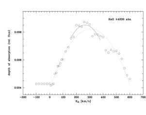
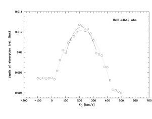
Figure 9: Measured depths of the absorption lines in the co-added spectra versus the assumed value for $K_{\rm O}$, shown for He ii $\lambda$4200 (upper) and He ii $\lambda$4542 (lower panel). Note the strong asymmetry. The parabolic fit is shown considering all data (dotted line) or only the central cusp (solid line). See text for more details.

In order to determine the value for $K_{\rm O}$ at which the absorption-line depth was maximal, a parabola was fitted to the data (see Figure 9). Comparing He ii $\lambda$4200 and He ii $\lambda$4542 immediately reveals that the strong asymmetry in He ii $\lambda$4200 leads to a position of the global maximum which is different from the value obtained from He ii $\lambda$4542, $(306\pm 69)$ versus $(217\pm 24)$ kms^-1. While technically, these two values are consistent with each other within their respective errors, we re-fitted both sets of points considering only the central cusp (fit shown in solid line). We now obtained $(265\pm 67)$ and $(214\pm 19)$ kms^-1 for He ii $\lambda$4200 and He ii $\lambda$4542, respectively. Since the error on the result for He ii $\lambda$4200 is $\sim 3.5$ times larger than for He ii $\lambda$4542, this leads to a very small relative weight ($\sim 1/12$), if one were to calculate a $\sigma$-weighted average. Furthermore, S08 reported that due to the lack of arc-comparison lines towards the blue end of their spectra, RV scatter was found to be larger than in the central region of the spectra (i.e., around He ii $\lambda$4686). Therefore, we did not calculate a weighted mean shift but rather entirely relied on the value obtained from the He ii $\lambda$4542 absorption. The second iteration yielded only a marginal change, $K_{\rm O}=(212\pm 19)$ kms^-1. The final, resulting O-star spectrum for the two absorption lines is shown in Figure 10.

Strong artifacts are present, possibly due to imperfect WR subtraction, not least because the WR emission lines display phase-dependent excess emission due to wind-wind collisions (see Section 3.6). Moreover, upon subtraction of the mean WR spectrum, slight misalignments between the WR mean and an individual spectrum will generate pseudo P Cyg profiles in the residuals, whose strength and width sensitively depend on the amount of misalignment; at least partially, these artifacts are reduced by the averaging process. Unfortunately, however, this effectively inhibits one to apply this method on the He ii $\lambda$4686 emission line, which would be much better visible than any absorption lines, should the secondary be an emission-line (e.g. an extreme Of/WN6) star as well.

The absorption lines of the putative secondary are very faint; the depth of the He ii $\lambda$4542 absorption line is $\sim$0.013 in units of relative flux, its ${\rm EW}=(60\pm 6)$ mÅ  (error estimated from results obtained for different continuum positions), and its ${\rm FWHM}=(5.4\pm 0.2)$ Å, the latter being consistent with what is to be expected from a typical O star. Given the extremely high S/N obtained in the co-added spectra (S/N $\sim$800), it is thus not implausible that these lines are indeed real. However, the low spectral resolution of our data, the frequent rebinning during the shift-and-add, errors in the orbital solution of the WR star, and noise will degrade the relatively narrow absorption lines of the O star, so the true depth might be somewhat larger. As an estimate, we adopt a degradation of the depth by a third, i.e. the true depth is 1.5 times larger than measured, i.e $\sim$0.02 relative flux. Comparing with the depth of the absorption lines He ii $\lambda$4200 and $\lambda$4542 in single, early-type O stars, which are typically 0.12 and 0.16 in continuum units, respectively (e.g., Walborn & Fitzpatrick 1990), we then find that the companion is diluted by a factor of at least $\sim$8; the WN6h component is thus at least $\sim$2.2 mag brighter than the O star. The same exercise can be repeated for the EW. Conti & Alschuler (1971) report a typical $\log{EW}(4542)=2.8\pm 0.1$, i.e. EW(4542) $\sim 630^{+170}_{-130}$ mÅ  for early-type O stars, with little variation between the spectral types. Using the above measure, we thus obtain a dilution factor $11^{+2}_{-3}$, consistent with what was derived above. At $\sim$same bolometric correction, this light ratio directly translates into a luminosity (and hence, mass) ratio. Using $L\propto M^{\alpha}$ with $\alpha=2$ yields the mass ratio of the system $q=M_{\rm WR}/M_{\rm O}=3.3^{+0.3}_{-0.5}$.

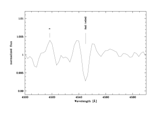
Figure 10: Co-added residual spectra for He ii $\lambda$4200 (upper) and He ii $\lambda$4542 (lower panel) after being shifted into the O-star’s frame of reference, using the best solution for $K_{\rm O}=212$ kms^-1 (see text for more details). The respective positions of the He ii absorption lines are indicated. Also indicated is an unidentified emission feature bluewards of He ii $\lambda$4542, which seems to be present in He ii $\lambda$4200 as well, but much less pronounced. Whether this feature is real or merely an artifact of the shift-and-add method, is unclear.

3.5 Masses of the Binary Components

To determine the absolute dynamical masses of both components in R145, we have averaged the values of the orbital parameters obtained for the two He ii lines $\lambda 4686$ and $\lambda 5411$ (cf. Table 5). With the usual relations

$$M_{1}\sin^{3}i=1.035\times 10^{-7}(K_{1}+K_{2})^{2}K_{2}P(1-e^{2})^{3/2}M_{\sun}$$

and

$$M_{2}\sin^{3}i=1.035\times 10^{-7}(K_{1}+K_{2})^{2}K_{1}P(1-e^{2})^{3/2}M_{\sun},$$

where $P$ is in days, $K$ in kms^-1, masses $M$ in solar units, and taking the values $K_{\rm WR}=(87\pm 21)$ kms^-1, $e=0.695\pm 0.028$, $P=(158.8\pm 0.1)$ days, and $K_{\rm O}=(212\pm 19)$ kms^-1 from the He ii $\lambda$4542 absorption (see above), we obtain minimum masses $M_{\rm WR}\sin^{3}i=(116\pm 33)$ M_☉ for the primary and $M_{\rm O}\sin^{3}i=(48\pm 20)$ M_☉ for the secondary. Thus, the mass ratio is $q=2.4\pm 1.2$, consistent with the value that was derived from the absorption-line strength (see above).

Although the uncertainties are large, minimum masses are already very high and consistent with R145’s absolute visual magnitude. From the BAT99 catalogue, $v=12.16$ mag and $b-v=0.03$. Adopting R144’s $(b-v)_{0}=-0.25$ (Crowther & Dessart 1998) for R145, we obtain $A_{v}\sim 0.87$ mag. With a distance modulus of $DM=18.5$ mag for the LMC and the relation $v-M_{v}=DM+A_{v}$, it follows that $M_{v}\sim-7.2$ mag, i.e. slightly brighter than that of WR20a, $M_{V}=-7.04$ mag (Rauw et al. 2007),

In WR20a, which consists of two equally massive, and hence equally bright, components, each one of the components has $M_{V}\sim-6.3$ mag. Since the light from R145 is entirely dominated by the WN6h component, the brightness difference between the WN6h component in R145 and one of the WN6ha components in WR20 is $\sim$0.9 mag; this brightness difference directly translates into a luminosity (and hence, mass) ratio. The flux ratio between the primary in R145 and one WN6ha component of WR20a is thus $\sim$2.3; assuming the same bolometric correction and $L\propto M^{2}$ yields a mass ratio of $\sim$1.5, i.e. $M_{\rm R145,WN6h}\sim 125M_{\sun}$. A different exponent in the mass-luminosity relation is possible, but covered by the large uncertainties on the stellar mass anyway, as are slight changes in reddening, intrinsic colors, and distance modulus.

At first glance, this result is in excellent agreement with the minimum mass obtained from the orbital motion. However, now the inclination angle has to be taken into account. The fit to the polarimetric data returns $i=38^{\circ}\pm 9^{\circ}$, $sin^{3}i=0.23^{+0.16}_{-0.12}$. Hence, the true masses of the binary components are higher by a factor $4.3^{+4.5}_{-1.8}$, at least 300 and 125 M_☉, respectively. Not only would such high masses be unprecedented, but R145 would also be severely underluminous for its mass. If the correct inclination angle were closer to 60^∘, the masses would still be $\sim$1.5 times higher, but then the resulting absolute masses would be roughly (if just) consistent with the intrinsic brightness of the system. However, the $\chi^{2}$ of the fit quickly deteriorates if the inclination angle is 10 to 15^∘ larger than the optimum value (see above), so there seems to be no margin for a significantly higher inclination angle.

Unless we accept that the polarimetry yields an entirely wrong inclination angle (which then would question the validity of the orbital solution altogether), the easiest way out is that the shift-and-add method is at fault, and that the secondary has a smaller RV amplitude, i.e. the mass (and hence, luminosity) ratio is smaller (A larger RV amplitude of the secondary would not remedy the situation, because the resulting system mass would be even higher, if everything else remained the same.) Then, however, the question arises why the secondary is not visible in the composite spectrum, let alone during the shift-and-add process. An explanation might be that the secondary itself is massive (luminous) enough to display a significant stellar wind, and resembles e.g. an extreme Of/WN6 star. The He ii $\lambda$4686 emission of such a star would be weak enough to be dominated by the much stronger line of the WN6h component, and possibly even be drowned out by excess emission arising from wind-wind collision in the residual spectra (see Section 3.6); on the other hand, the He ii $\lambda$4200 and $\lambda$4542 absorptions could (at least partially) be filled up by wind emission. The latter would seriously affect the usefulness of measuring the depth or the EW of the absorption lines in the co-added residuals (any further challenges with this notwithstanding, see above), and entirely falsify the luminosity (and hence, mass) ratio that was derived from the absorption-line strengths, etc. In the following section, we will therefore use an independent approach to obtain an estimate on the inclination angle.

3.6 Wind-Wind Interaction Effects

As mentioned above, it is well known that in WR+O binaries, where both stars have strong winds, WWCs occur which generate two cone-shaped shocks separated by a contact discontinuity. This contact discontinuity wraps around the star with the weaker wind (i.e. that with less wind momentum), which is usually the O star. As the shocked matter flows with high velocities downstream along the contact discontinuity, it cools, giving rise to excess emissions which can be seen atop some optical emission lines of the WR star. The position of the excess bumps atop the emission lines depends on the orientation of the flow. The shock-cone acts like a beacon of a lighthouse: if it is pointing towards the observer, the excess emission will be blue-shifted, and half an orbit later, the matter will be flowing away from the observer, resulting in a red-shifted excess emission. Due to the orbital motion, the Coriolis force will slightly distort the cone, tilting its axis and making it curve away at large separations, with respect to the line of sight between the WR and the O star.

To study this behavior in more detail in R145, all spectra were shifted into the rest frame of the WR star. Then, a minimum spectrum was computed by averaging spectra obtained near apastron, i.e. around $\phi\sim 0.5$, when the WWC excess emissions are weakest. (While the excess emissions are not zero, as will be shown below, differences remain small and have no influence on the conclusions drawn here.) Due to the eccentricity of the orbit, phases near apastron are well covered, and a good-quality minimum spectrum was obtained. The minimum was subtracted from all spectra of the time series, the residuals were shifted back into the observer’s frame of reference, folded into the corresponding phase of the binary period, and a dynamic spectrum was constructed where the intensities are coded in greyscales, white being the strongest emission. Forty phase-bins were used for good resolution, covering one orbital cycle centered on $\phi=0$, at which periastron passage occurs. The result is shown in Figure 11.

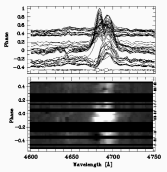
Figure 11: Overplot (upper panel) and greyscale (lower panel) of the residual spectra in the observer’s frame of reference, after subtraction of the minimum profile. While the He ii $\lambda$4686 emission line is highly variable, the strongest increase occurs around periastron passage ($\phi=0$). The WR star passes in front at $\phi=0.5$ and it can (if just) be seen that it is at this phase that the WWC excess emission displays the largest redshift. Horizontal black stripes in the greyscale correspond to empty phase bins.

Since the WWC excess emissions vary in shape and position over the orbital cycle in a defined way, modelling their profile can be used to obtain an independent measure of the system parameters like e.g. the orbital inclination (see Luehrs 1997). Unfortunately, the quality of our data is not sufficient to grant such an analysis, but a simplified method was developed by Hill et al. (2000) that still allows one to obtain valuable information from the phase dependency of the excess emission.

Following Hill et al.’s (2000) approach, we have measured the full-width at half maximum (FWHM) and the mean RV of the excess-emission profiles, i.e. of the residuals after having subtracted the minimum spectrum (see above). These values follow the relation

$${\rm FWHM} = C_{1}+2v_{\rm cone}\sin\theta\sqrt{1-\sin^{2}i\cos^{2}(\phi-\delta\phi)}$$

$${\rm RV} = C_{2}+v_{\rm cone}\cos\theta\sin i\cos(\phi-\delta\phi),$$

with $C_{1}$ and $C_{2}$ simple constants, $v_{\rm cone}$ the stream velocity along the shock cone, $\theta$ the half opening angle of the cone, $\phi$ the respective orbital phase, $\delta\phi$ the tilt angle of the cone axis due to the Coriolis force which leads to a phase shift between the orbital and the cone motion, and $i$ the orbital inclination angle (also see Fig. 6 of Hill et al. 2000). A constraint is that the stream velocity in the cone must not exceed the wind terminal velocity (1300 kms^-1, see Section 3.7). A least-square fit to the data is shown in Figure 12. It is satisfactory for the FWHM, but less so for the mean RV, most likely to insufficient data quality. We obtain $C_{1}=30$ kms^-1, $C_{2}=220$ kms^-1, $v_{\rm cone}=810$ kms^-1, $\theta=69^{\circ}$, and $\delta\phi=0$. The inclination angle is found to be $i=45^{\circ}$, in excellent agreement with the result obtained by polarimetry. Just as in the case of the polarimetry (see above), a fit with $i=90^{\circ}$ is ruled out by the data; thus it appears that R145 is indeed seen under such a low inclination, with the consequences discussed above.

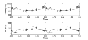
Figure 12: Fit to the FWHM (upper panel) and mean RV (lower panel) of the WWC excess-emission profile. See text for more details.

As can be seen from Figure 11, the WWC excess emission is by far strongest at periastron passage, i.e. when the two stars are closest to each other, and quickly drops when the separation between the stars increases. The dependence of the excess emission on the separation can be studied in more detail, using the recipe by Stevens et al. (1992). These authors have shown that the WWC zone of relatively wide binaries can be treated as adiabatic, even at periastron; therefore the amount of X-ray flux generated by WWC is expected to go with the inverse separation between the stars (also see Usov 1992). Since He ii $\lambda$4686 is a recombination line (i.e. formed through “collision” of two particles) the formalism of Stevens et al. (1992) can be applied to the strength of the excess emission, too. Assuming the WWC excess emission in He ii $\lambda$4686 to be optically thin, we can thus expect a rise and fall of the emissitivity which is $\propto D^{-1}$, where $D$ is the separation between the WR and the O star. We here use the relative separation $D(v)$ as a function of true anomaly $v$, normalized by the minimum separation $d_{\rm min}$, i.e.

$$D(v)=d(v)/d_{\rm min}=\frac{1+e}{1+e\cos v},$$

where $v$ is the true anomaly of the orbital ellipse and $D_{\rm min}=1$ at periastron ($v=0$, phase of the elliptical orbit $\phi=0$), and consequently $D_{\rm max}=(1+e)/(1-e)$ at apastron ($v=\pi$, $\phi=0.5$). Note that due to this normalization, the expression is independent of the inclination angle. However, while the excess emission is minimum at apastron, it is not generally zero. Thus, the observed EW of the He ii $\lambda$4686 emission is at any time the sum of the EW of the unperturbed WR emission, $E_{0}$, and a separation-dependent excess flux, $X_{0}/D(v)$, so that $EW(D)=E_{0}+X_{0}/D(v)$, with $X_{0}$ a constant (the maximum excess), and $D(v)$ as defined above. For verification, we also fitted a steeper dependency, $EW^{\prime}(D)=E^{\prime}_{0}+X^{\prime}_{0}/D(v)^{2}$.

From equal-weight least-square fitting, we obtained pairs of $(E_{0};X_{0})=(49.2;13.4)$ for the $1/D$ dependency, and $(E^{\prime}_{0};X^{\prime}_{0})=(51.8;11.4)$ for the $1/D^{2}$ case (EWs in Å). The data are shown in Figure 13, with the two theoretical curves overplotted. While both curves certainly look equally well-fitting, the $1/D^{2}$ curve yields a $\chi^{2}$ that is $\sim$10% larger than that for the $1/D$ case. Since our data are rather noisy, and show larger scatter around periastron than around apastron, it is difficult to assess the true (a posteriori) measurement error per individual data point. Using the scatter of the data around apastron for this, the normalized $\chi{2}$ of the fit is $\sim$2, but larger if the scatter around periastron is adopted.

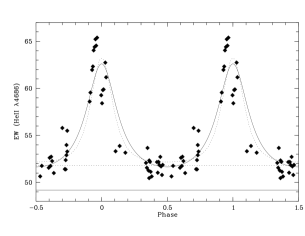
Figure 13: Equivalent widths of the He ii $\lambda$4686 emission as a function of orbital phase (i.e. separation $D$). Overplotted are the hypothetical emissivity curves; the solid line represents an emissivity rising and falling with $D^{-1}$, whereas the dotted line is for a steeper $D^{-2}$ law. The horizontal lines indicate the unperturbed equivalent width, as obtained from the fit for the $D^{-1}$ case (solid line) and the $D^{-2}$ case (dotted line). See text for more details.

3.7 The Mass-Loss Rate of the WN Star

Independent of any issues regarding the orbital inclination angle, we can obtain a rough estimate of the mass-loss rate, $\dot{M}_{\rm WR}$, of the WN6h star in R145, assuming that the companion has a negligible mass loss. Following the prescription of Moffat et al. (1998; also see references therein), we use the total optical depth in polarization due to electron scattering

$$\tau=23\sigma_{T}f_{c}\dot{M}_{\rm WR}(1+\cos^{2}i)\sin i/[(16\pi)^{2}m_{p}v_{\infty}a],$$

where $\sigma_{T}$ is the Thomson electron-scattering cross-section, $f_{c}=I_{\rm O}/(I_{\rm WR}+I_{\rm O})$ the intensity ratio between the O star and the total luminosity, $m_{p}$ the proton mass, $v_{\infty}$ the wind terminal velocity, and $a=[P^{2}(M_{\rm WR}+M_{\rm O})]^{1/3}$ the orbital separation. For $f_{c}$, we use the light ratio $\sim 0.125$ as derived above from the absorption-line strength of the O star companion with respect to single early-type O stars. From tailored atmosphere analysis of R144, Crowther & Dessart (1998) found $v_{\infty}=1350$ kms^-1. S08 report that the FWHM of the He ii $\lambda$4686 emission line in R145 is only slightly smaller than in R144; assuming that both stars are similar enough that the FWHM of He ii $\lambda$4686 can act as a reasonable proxy of the terminal wind velocity, we adopt for R145 a value of $v_{\infty}=1300$ kms^-1. For $i$ and $\tau$, the averaged values from Table 5 are taken.

Inserting those values in the equation given above yields a very high mass-loss rate of $\dot{M}_{\rm WR}=1.0\times 10^{-4}$ M_☉yr^-1 (remarkably, for inclination angles between $40^{\circ}$ and $90^{\circ}$ this value changes barely). From tailored analysis and using models without iron-line blanketing and wind clumping, Crowther & Dessart (1998) found $\dot{M}=1.5\times 10^{-4}$ M_☉yr^-1 for R144. Introducing typical clumping factors $f\sim 0.1$ usually reduces the mass-loss rates derived from spectroscopic means by a factor of $1/\sqrt{f}\sim 3$, i.e. to more sensible $\dot{M}=5\times 10^{-5}$ M_☉yr^-1; since R144 is the more luminous star of the two, one would expect an even lower mass-loss rate for R145. However, since polarization depends only on the number of scatterers (i.e. electrons), polarimetric diagnostics are unaffected by wind clumping, and polarization is indeed observed to be that high in R145.

Thus, assuming the models to be correct, such a high, continuous mass-loss rate for R145 would be sensible only if the wind were particularly smooth. Another way to lower the derived mass-loss rate would be to considerably decrease the orbital separation $a$ or the terminal wind speed $v_{\infty}$. The former would require a mass-ratio closer to unity, with the consequences discussed above, while the latter is unlikely, given the close resemblance of R145 to R144. We thus conclude that the primary of R145 may in fact have a very high mass-loss rate, subject to further confirmation.

4 Summary and Conclusion

We have combined previously published radial velocity (RV) data from Moffat (1989) with data obtained by Schnurr et al. (2008b), along with previously unpublished polarimetric data, for the two WN6h stars R144 and R145 in the LMC. While the former star was first suspected to be binary by Schnurr et al. (2008b), the latter had already been identified as a binary by Moffat (1989).

While our study could not reveal any periodicity in the data of R144, we have, for the first time, established the full set of orbital parameters for R145. The orbital period was found to be $P=(158.8\pm 0.1)$ days, in contrast to the preliminary estimate of 25.4 days by Moffat (1989), based on the assumption of a circular orbit. From our analysis of the polarimetric data for R145, the inclination angle of the orbital system was found to be very low, $i=38^{\circ}\pm 9^{\circ}$. This value was confirmed by a simplified study of the phase-dependent excess emission on the He ii $\lambda$4686 line due to wind-wind collision. Following the approach of Hill et al. (2000), we obtained a consistent value of $i=45^{\circ}$.

By applying a modified version of the shift-and-add method originally developed by Demers et al. (2002), we were able to isolate the spectral signature of the O-star companion. We found the RV amplitude of the primary (WN) star to be $K_{\rm WN}=(87\pm 21)$ kms^-1, while the RV amplitude of the secondary (O) star was found to be $K_{\rm O}=(212\pm 19)$ kms^-1. We derived the minimum masses of the WR and the O component to be, respectively, $M_{\rm WN}\sin^{3}i=(116\pm 33)$ M_☉ and $M_{\rm O}\sin^{3}i=(48\pm 20)$ M_☉. While the large mass ratio $q=M_{\rm WR}/M_{\rm O}\sim 2.4\pm 1.2$ is compatible with the strong dilution of the O-companion’s absorption lines, the absolute masses of the two stars are problematic. If the derived, low inclination angle is correct, one obtains minimum absolute masses of 300 and 125 M_☉ for the WN and the O star, respectively, but such high masses are not compatible with the observed luminosity of R145, which puts the system between NGC3603-A1 (see Schnurr et al. 2008a) and WR20a (Rauw et al. 2007). Given that both NGC3603-A1 and WR20a consist of two $\sim$equally bright stars, while in R145 the WN component dominates the light, masses of 120 and 50 M_☉ are more likely, but this would require an inclination angle close to 90^∘, which is not supported by the data. Another possibility, the mass ratio being closer to unity, is not supported by the results of the shift-and-add method. Thus, something is clearly odd in R145, and more and better data are required.

From the polarimetric data for R145, we also estimated a rather extreme value of the mass-loss rate for the WR component, of $\sim 10^{-4}$ M_☉yr^-1, which is suspiciously high even for such a massive and hence luminous object. Analyzing the He ii $\lambda$4686 excess emission from wind-wind collisions in R145, we find that its strength depends on the separation $d$ of the two stars as $d^{-1}$, as is expected from theory of adiabatic winds, but that a steeper dependence, $\propto d^{-2}$, which was reported for WR140 by Marchenko et al. (2003), cannot unambiguously be ruled out.

Given the very large uncertainties on the values derived from our data, our findings cannot be considered other than preliminary. However, given the fact that R145 seems to contain one of the most luminous and thus probably also most massive stars known in the Local Group, we feel that any additional effort is well deserved to obtain more reliable results. Therefore, we are currently carrying out a long-term monitoring of this system, along with R144, but we strongly encourage independent studies of these potential cornerstone objects.

References

- Aspin et al. (1981) Aspin C., Simmons J. F. L., Brown J. C., 1981, MNRAS, 194, 283
- Bonanos et al. (2004) Bonanos A. Z., Stanek K. Z., Udalski A., Wyrzykowski L., Żebruń K., Kubiak M., Szymański M. K., Szewczyk O., Pietrzyński G., Soszyński I., 2004, ApJ, 611, L33
- Brown et al. (1982) Brown J. C., Aspin C., Simmons J. F. L., McLean I. S., 1982, MNRAS, 198, 787
- Conti & Alschuler (1971) Conti P. S., Alschuler W. R., 1971, ApJ, 170, 325
- Crowther & Dessart (1998) Crowther P. A., Dessart L., 1998, MNRAS, 296, 622
- de Koter et al. (1997) de Koter A., Heap S. R., Hubeny I., 1997, ApJ, 477, 792
- Demers et al. (2002) Demers H., Moffat A. F. J., Marchenko S. V., Gayley K. G., Morel T., 2002, ApJ, 577, 409
- Figer (2005) Figer D. F., 2005, Nat, 434, 192
- Foellmi et al. (2003) Foellmi C., Moffat A. F. J., Guerrero M. A., 2003, MNRAS, 338, 360
- Harries & Howarth (1996) Harries T. J., Howarth I. D., 1996, A&A, 310, 235
- Hill et al. (2000) Hill G. M., Moffat A. F. J., St-Louis N., Bartzakos P., 2000, MNRAS, 318, 402
- Hillier (1988) Hillier D. J., 1988, ApJ, 327, 822
- Hillier (1989) Hillier D. J., 1989, ApJ, 347, 392
- Kim et al. (1998) Kim S., Staveley-Smith L., Dopita M. A., Freeman K. C., Sault R. J., Kesteven M. J., McConnell D., 1998, ApJ, 503, 674
- Luehrs (1997) Luehrs S., 1997, PASP, 109, 504
- Magalhaes et al. (1984) Magalhaes A. M., Benedetti E., Roland E. H., 1984, PASP, 96, 383
- Marchenko et al. (2003) Marchenko S. V., Moffat A. F. J., Ballereau D., Chauville J., Zorec J., Hill G. M., Annuk K., Corral L. J., Demers H., Eenens P. R. J., Panov K. P., Seggewiss W., Thomson J. R., Villar-Sbaffi A., 2003, ApJ, 596, 1295
- Moffat (1989) Moffat A. F. J., 1989, ApJ, 347, 373
- Moffat et al. (1998) Moffat A. F. J., Marchenko S. V., Bartzakos P., Niemela V. S., Cerruti M. A., Magalhaes A. M., Balona L., St-Louis N., Seggewiss W., Lamontagne R., 1998, ApJ, 497, 896
- Moffat & Seggewiss (1979) Moffat A. F. J., Seggewiss W., 1979, A&A, 77, 128
- Nakamura & Umemura (2001) Nakamura F., Umemura M., 2001, ApJ, 548, 19
- Niemela et al. (2008) Niemela V. S., Gamen R. C., Barbá R. H., Fernández Lajús E., Benaglia P., Solivella G. R., Reig P., Coe M. J., 2008, MNRAS, 389, 1447
- Ostriker & Gnedin (1996) Ostriker J. P., Gnedin N. Y., 1996, ApJ, 472, L63+
- Rauw et al. (2004) Rauw G., De Becker M., Nazé Y., Crowther P. A., Gosset E., Sana H., van der Hucht K. A., Vreux J.-M., Williams P. M., 2004, A&A, 420, L9
- Rauw et al. (2007) Rauw G., Manfroid J., Gosset E., Nazé Y., Sana H., De Becker M., Foellmi C., Moffat A. F. J., 2007, A&A, 463, 981
- Rauw et al. (1996) Rauw G., Vreux J.-M., Gosset E., Hutsemekers D., Magain P., Rochowicz K., 1996, A&A, 306, 771
- Robert et al. (1992) Robert C., Moffat A. F. J., Drissen L., Lamontagne R., Seggewiss W., Niemela V. S., Cerruti M. A., Barrett P., Bailey J., Garcia J., Tapia S., 1992, ApJ, 397, 277
- Schaerer (2002) Schaerer D., 2002, A&A, 382, 28
- Schnurr et al. (2008a) Schnurr O., Casoli J., Chené A.-N., Moffat A. F. J., St-Louis N., 2008a, MNRAS, 389, L38
- Schnurr et al. (2008b) Schnurr O., Moffat A. F. J., St-Louis N., Morrell N. I., Guerrero M. A., 2008b, MNRAS, 389, 806
- Schweickhardt et al. (1999) Schweickhardt J., Schmutz W., Stahl O., Szeifert T., Wolf B., 1999, A&A, 347, 127
- Simmons et al. (1982) Simmons J. F. L., Aspin C., Brown J. C., 1982, MNRAS, 198, 45
- Simmons & Boyle (1984) Simmons J. F. L., Boyle C. B., 1984, A&A, 134, 368
- Stahl et al. (1986) Stahl O., Buzzoni B., Kraus G., Schwarz H., Metz K., Roth M., 1986, The Messenger, 46, 23
- Stellingwerf (1978) Stellingwerf R. F., 1978, ApJ, 224, 953
- Stevens et al. (1992) Stevens I. R., Blondin J. M., Pollock A. M. T., 1992, ApJ, 386, 265
- Usov (1992) Usov V. V., 1992, ApJ, 389, 635
- Villar-Sbaffi et al. (2006) Villar-Sbaffi A., St-Louis N., Moffat A. F. J., Piirola V., 2006, ApJ, 640, 995
- Walborn & Fitzpatrick (1990) Walborn N. R., Fitzpatrick E. L., 1990, PASP, 102, 379
- Weidner & Kroupa (2004) Weidner C., Kroupa P., 2004, MNRAS, 348, 187
- Wolinski & Dolan (1994) Wolinski K. G., Dolan J. F., 1994, MNRAS, 267, 5