Evaporation induced flow inside circular wells

Abstract

Flow field and height averaged radial velocity inside a droplet evaporating in an open circular well were calculated for different modes of liquid evaporation.

1 Introduction

Wide used technique of patterning surfaces with solid particles utilizes the evaporation of colloidal droplets from a substrate. In particular, evaporation of liquid samples is a key problem in the development of microarray technology (including labs-on-a chip), especially in the case of open reactors Rieger .

A plenty of works are devoted to the evaporation of the sessile droplets Deegan_2000 ; Fischer_2002 ; Mollaret_2004 ; Hu_2005 . One assumes that a droplet has a shape like a spherical cap. Nevertheless, investigation of the drops with more complex geometry is of interest. Thus when a high concentrated colloidal droplet evaporates from a substrate, the solute particles in solution will form a ring like deposit wall near the edge of the drop (Fig. 1). One can consider this case as evaporation of a liquid drop inside open circular well with vertical walls formed by gel.

Figure 1: Time evolution of the deposit phase growth Popov_2005

In the paper Rieger the flow field inside a liquid sample in very thin circular wells was measured. The confidence between measured velocity Rieger and the estimations obtained with theory of ring formation Deegan_2000 is reasonable.

In this paper, the relationship between hydrodynamical flow inside a liquid sample evaporating in open circular well and the mode of evaporation is examined.

We found analytical expressions of height averaged radial velocity for different modes of evaporation. Velocity field inside the circular well was found for the particular case of flat air–liquid interface.

2 Velocity field inside circular well

2.1 Height averaged radial velocity

We will consider one particular but interesting case, because of its practical applications, when a liquid inside a circular well may be described as a thin film. So, in paper Rieger in circular wells with a radius of $r_{f}=100$ $\mu$m and a depth of $h_{f}=6$ $\mu$m were investigated. Approximately the same ratio depth to radius is typical for the drops of biological fluids used for medical tests Savina_1999 ; Shabalin_2001 .

Moreover, we will suppose that evaporation is a steady state process. This assumption is valid e.g. for evaporation of the drops of aqueous solutions under room temperature and normal atmosphere pressure, i.e. for the typical experimental conditions. Apex dynamics is rather slow Rieger

$$H(t)=(7.38\mathrm{\mu m}-6.13\mathrm{\mu m})-(0.042\mathrm{\mu m/s})t.$$

In the cases of medical tests, the typical velocity of drop apex is approximately 1 mm/h.

Mass conservation gives the following equation for height averaged radial velocity Deegan_2000

$$\langle v_{r}(r,t)\rangle=\\ -\frac{1}{\rho rh}\int\limits_{0}^{r}\left(j(r,t)\sqrt{1+\left(\frac{\partial h}{\partial r}\right)^{2}}+\rho\frac{\partial h}{\partial t}\right)r\,dr,$$ (1)

where $h=h(r,t)$ is the drop shape, $\rho$ is the density of solution, $j(r,t)$ is the evaporation rate defined as the evaporative mass loss per unit surface area per unit time.

Considering the thin droplets only ($h(r,t)\ll r_{f})$ we will neglect everywhere $h^{2}(0,t)$ and $\left(\frac{\partial h}{\partial r}\right)^{2}$ in compare with 1. We will utilize approximative equation for air–liquid interface

$$h(r,t)=h(0,t)\left(1-\left(\frac{r}{r_{f}}\right)^{2}\right),$$ (2)

where $r_{f}$ is radius of circular well.

Since the drop is thin and the contact angle is small, we will use the expression

$$j(r)=\frac{j_{0}}{\sqrt{1-\left(\frac{r}{r_{f}}\right)^{2}}}$$ (3)

for the evaporation rate, which has a reciprocal square-root divergence near the contact line Popov_2005 . This expression can be derived from Laplace equation (see Deegan_2000 ; Popov_2005 for details). This functional form for vapor flux is widely used, in particular, it was utilized in paper Rieger .

Some quantities of interest can be expressed analytically exploiting (3). Velocity of drop apex decrease is

$$\frac{dh(0,t)}{dt}=-\frac{4j_{0}}{\rho}.$$ (4)

Height averaged radial velocity is

$$\langle v_{r}(x,t)\rangle=-\frac{j_{0}\left(1-\sqrt{1-x^{2}}-2x^{2}+x^{4}\right)}{\rho x(h_{0}+L(0,t)(1-x^{2}))},$$ (5)

where $x=\frac{r}{r_{f}}$, $L=\frac{h}{r_{f}}$, $h_{0}=\frac{h_{f}}{r_{f}}$. $h_{f}$ is the height of vertical wall of the well.

Exploiting of Eq. 3 leads to a singularity for both vapor flux and gradient of the height averaged velocity of liquid inside a drop at the edge of droplet. A smoothing function may be used to eliminate physically senseless divergency Cachile_2002

$$j(x,t)=\frac{j_{0}}{r_{f}\sqrt{1-x^{2}}}\frac{1-\exp(-m\sqrt{1-x^{2}})}{1-\exp(-m)},$$ (6)

where $m$ is an adjustable constant. In this case, height averaged radial velocity can be written analytically

$$\langle v_{r}(x,t)\rangle=\frac{j_{0}}{x(h_{0}+L\left(x,t\right))m\left(1-{{\rm e}^{-m}}\right)}\times\\ \left(m\sqrt{1-x^{2}}+{{\rm e}^{-m\sqrt{1-{x}^{2}}}}-m-{{\rm e}^{-m}}-\phantom{\frac{x^{2}}{2}}\right.\\ \left.2\,\left(1-m-{{\rm e}^{-m}}\right)\left(1-\frac{x^{2}}{2}\right)x^{2}\right),$$ (7)

where $L(x,t)=\left(L(0,0)+4{\frac{{j_{0}}\,\left(1-m-{{\rm e}^{-m}}\right)t}{m\left(1-{{\rm e}^{-m}}\right)}}\right)\left(1-x^{2}\right).$

Another evaporative flux functions was proposed in Anderson_1995

$$j(x,\tau)=\frac{j_{0}}{K+L(x,\tau)},$$ (8)

where the constant $K$ measures the degree of non-equilibrium at the evaporating interface and is related to material properties. $K\to 0$ corresponds to a highly volatile droplet. The limit $K\to\infty$ corresponds to a nonvolatile droplet. Analytical expression for height averaged velocity inside circular well can be obtained if vapor flux is described by Eq. 8

$$\langle v_{r}(x,t)\rangle=\frac{j_{0}}{2x\left(h_{0}+L(0,t)(1-x^{2})\right)}\times\\ \times\left(\frac{1}{L(0,t)}\ln\left(1-\frac{L(0,t)x^{2}}{K+h_{0}+L(0,t)}\right)-\right.\\ \left.\frac{x^{2}\left(1-\frac{x^{2}}{2}\right)\left(L(0,t)-2(K+h_{0})\right)}{\left(K+h_{0}\right)^{2}}\right),$$ (9)

where $L(0,t)=2(K+h_{0})+(L_{0}-2(K+h_{0}))\exp\left(\frac{j_{0}t}{(K+h_{0})^{2}}\right).$

Deegan et al. Deegan_2000 demonstrated experimentally, that if evaporation is greatest at the center of the droplet, a uniform distribution of colloidal particles remained on the substrate. Simulations by Fischer_2002 confirmed, that as fluid is lost from the center of the droplet, an inward flow develops to replenish the evaporated fluid. The evaporative flux function was proposed by Fischer Fischer_2002 to mimic evaporation that is concentrated at the center of the droplet

$$j(x,t)=\frac{j_{0}}{L(0,t)}\mathrm{e}^{-Ax^{2}},$$ (10)

where $A$ is an adjustable constant.

We derived the analytical expression for height averaged velocity for evaporation function given by Eq. 10

$$\langle v_{r}(x,t)\rangle=\\ \frac{j_{0}\left(1-{{\rm e}^{-Ax^{2}}}+\left(1-{{\rm e}^{-A}}\right)x^{2}\left(x^{2}-2\right)\right)}{2Ax(h_{0}+L(x,t))L(0,t)},$$ (11)

where

$$L(x,t)=\\ \left(1-x^{2}\right)\left(\sqrt{\left(h_{0}+L_{0}\right)^{2}-4\frac{j_{0}\,\left(1-{\rm e}^{-A}\right)t}{A}}-h_{0}\right).$$

Fig. 2 demonstrates our calculations for all described above evaporative functions. In all figures, the plots corresponds to: initial stage (air–liquid interface is convex); air–liquid interface is flat; air–liquid interface is concave with the same curvature as at the initial stage; 90 % of time, when air–liquid interface touch the bottom of the well.

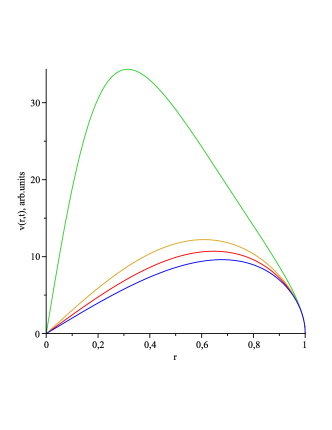
a) b)
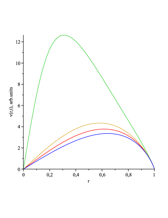
c) d)

Figure 2: Height averaged radial velocity for different modes of evaporation: a) (3); b) (6) if $m=5$; c) (8); d) (10). For additional explanations see the main text.

2.2 Velocity field

Velocity fields calculated for sessile droplets from Laplace equation Tarasevich2005 and from Navier–Stokes equations Fischer_2002 are very similar. We hope that ideal liquid is reasonable assumption for our object of interest.

Cylindrical coordinates $(r,\varphi,z)$ will be used, as they are most natural for the geometry of interest. The origin is chosen in the center of the circular well on the substrate. The coordinate $z$ is normal to the substrate, and the bottom of the circular well is described by $z=0$, with $z$ being positive on the droplet side of the space. The coordinates $(r,\varphi)$ are the polar radius and the angle, respectively. Due to the axial symmetry of the problem and our choice of the coordinates, no quantity depends on the angle $\varphi$, in particular $u=u(r,z)$.

The mass flux at the vertical wall of circular well is absent, hence

$$\left.\frac{\partial u}{\partial r}\right|_{r=r_{f}}=0,$$ (12)

where $r_{f}$ is radius of the circular well.

Moreover, there is physically obvious relation

$$\left.\frac{\partial u}{\partial r}\right|_{r=0}=0.$$ (13)

The bottom of the circular well is impermeable, hence

$$\left.\frac{\partial u}{\partial z}\right|_{z=0}=0.$$ (14)

The mass flux inside the droplet near the air–liquid interface $f(r)$ is connected with vapor flux

$$\left.\frac{\partial u}{\partial z}\right|_{\text{free surface}}=f(r).$$ (15)

Laplace equation in cylindrical coordinates for the axially symmetric case is written as

$$\frac{1}{r}\frac{\partial}{\partial r}\left(r\frac{\partial u}{\partial r}\right)+\frac{\partial^{2}u}{\partial z^{2}}=0.$$ (16)

Boundary problem (12),(14), for equation (16)

$$u(r,z)=\sum\limits_{n=1}^{\infty}a_{n}\cosh\left(\frac{\mu_{n}^{(1)}}{r_{f}}z\right)J_{0}\left(\frac{\mu_{n}^{(1)}}{r_{f}}r\right),$$ (17)

where $J_{m}(r)$ is the Bessel function of the first kind, order $m$, $\mu_{n}^{(1)}$ are the real zeros of Bessel $J_{1}(r)$ function: $J_{1}(r)=0$. Note that condition (13) is satisfied automatically.

Taking into account relation between velocity and potential $\vec{v}=-\operatorname*{grad}u$, we can find radial component of velocity

$$\langle v_{r}(r,z)\rangle=\sum\limits_{n=1}^{\infty}a_{n}\cosh\left(\frac{\mu_{n}^{(1)}}{r_{f}}z\right)\frac{\mu_{n}^{(1)}}{r_{f}}J_{1}\left(\frac{\mu_{n}^{(1)}}{r_{f}}r\right).$$

Height averaged radial velocity, i.e. the same velocity examined in Rieger , can be written as

$$\langle v_{r}(r)\rangle=\frac{1}{h_{f}}\int\limits_{0}^{h_{f}}v_{r}(r,z)\,dz=\\ \frac{1}{h_{f}}\sum\limits_{n=1}^{\infty}a_{n}\sinh\left(\frac{\mu_{n}^{(1)}}{r_{f}}h_{f}\right)J_{1}\left(\frac{\mu_{n}^{(1)}}{r_{f}}r\right).$$

Coefficients $a_{n}$ can be obtained from (15). For simplicity we will assume that air–liquid interface is flat.

$$\left.\frac{\partial u}{\partial z}\right|_{z=h_{f}}=\\ \sum\limits_{n=1}^{\infty}a_{n}\frac{\mu_{n}^{(1)}}{r_{f}}\sinh\left(\frac{\mu_{n}^{(1)}}{r_{f}}h_{f}\right)J_{0}\left(\frac{\mu_{n}^{(1)}}{r_{f}}r\right)=f(r).$$ (18)

We introduce notation

$$\int f(r)r\,dr=F(r).$$

$$\sum\limits_{n=1}^{\infty}c_{n}J_{1}\left(\frac{\mu_{n}^{(1)}}{r_{f}}r\right)=\frac{F(r)}{r}$$ (19)

is a Fourier–Bessel series of $F(r)/r$, where

$$c_{n}=a_{n}\sinh\left(\frac{\mu_{n}^{(1)}}{r_{f}}h_{f}\right).$$ (20)

Hence,

$$a_{n}=\\ \frac{2}{r_{f}^{2}\sinh\left(\frac{\mu_{n}^{(1)}}{r_{f}}h_{f}\right)J_{0}^{2}\left(\mu_{n}^{(1)}\right)}\int\limits_{0}^{r_{f}}J_{1}\left(\frac{\mu_{n}^{(1)}}{r_{f}}r\right)F(r)\,dr.$$ (21)

We need to determine $f(r)$ to find the unknown coefficients.

Mass conservation leads to the relation

$$\left.\frac{\partial u}{\partial z}\right|_{z=h_{f}}=-\frac{\partial L(r,t)}{\partial t}-\frac{J(r,t)}{\rho}.$$ (22)

We computed velocity fields for all evaporation laws described in Sec. 2.1. The results show that current inside circular well is horizontal excluding rather narrow region near the wall and in the center of the well for the case of practical interest ($h/r\sim 0.1$).

Many authors supposed that evaporation induced flow inside the droplets is independent of its height. Our simulations confirmed validity of this very wide used approach for thin droplets.

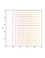
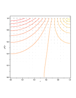
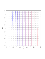
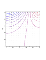
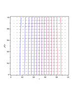
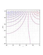
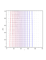
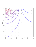
Figure 3: Velocity field inside circular well for differen evaporative modes. The air–liquid interface is supposed to be flat. From top to bottom (3), (6) with $m=5$, (8), (10). Left column corresponds to ratio $h_{f}/r_{f}=0.0618$, right column corresponds to ratio $h_{f}/r_{f}=0.99$

- (1) B. Rieger, L. R. van den Doel, L. J. van Vliet, Physical Review E 68, 036312 (2003).
- (2) R. D. Deegan, O. Bakajin, T. F. Dupont, G. Huber, S. R. Nagel, T. A. Witten, Phys. Rev. E 62, 756 (2000)
- (3) B. J. Fischer, Langmuir 18, 60 (2002)
- (4) R. Mollaret, K. Sefiane, J. R. E. Christy, D. Veyret, Chem. Eng. Res. Design 82(A4), 471 (2004)
- (5) H. Hu, R. G. Larson, Langmuir 21, 3963 (2005)
- (6) Y. O. Popov, Phys. Rev. E 71, 036313 (2005)
- (7) L. V. Savina, Crystaloscopical structures of blood serum of healthy and seek human (Sovyetskaya Kuban, Krasnodar, 1999)
- (8) V. N. Shabalin, S. N. Shatokhina, Morphology of Biological Fluids (Khrizostom, Moscow, 2001)
- (9) M. Cachile, O. Bénichou, A. M. Cazabat, Langmuir 18, 7985 (2002)
- (10) D. M. Anderson, D. M. Davis, Physics of Fluids 7, 248 (1995)
- (11) Y. Y. Tarasevich, Phys. Rev. E 71, 027301 (2005)