A Metric and Optimisation Scheme for Microlens Planet Searches

Abstract

OGLE III and MOA-II are discovering 600-1000 Galactic Bulge microlens events each year. This stretches the resources available for intensive follow-up monitoring of the lightcurves in search of anomalies caused by planets near the lens stars. We advocate optimizing microlens planet searches by using an automatic prioritization algorithm based on the planet detection zone area probed by each new data point. This optimization scheme takes account of the telescope and detector characteristics, observing overheads, sky conditions, and the time available for observing on each night. The predicted brightness and magnification of each microlens target is estimated by fitting to available data points. The optimisation scheme then yields a decision on which targets to observe and which to skip, and a recommended exposure time for each target, designed to maximize the planet detection capability of the observations. The optimal strategy maximizes detection of planet anomalies, and must be coupled with rapid data reduction to trigger continuous follow-up of anomalies that are thereby found. A web interface makes the scheme available for use by human or robotic observers at any telescope. We also outline a possible self-organising scheme that may be suitable for coordination of microlens observations by a heterogeneous telescope network.

1 Introduction

Gravitational microlensing reveals stars and planets that magnify the light from a background source star [Mao & Paczynski 1991]. The wide-field OGLE III [Udalski, et al. 2003] and MOA II surveys of Galactic Bulge starfields discover $\sim 600-1000$ microlensing events each year. During these events, a background source star brightens and fades, sometimes by many magnitudes, in $t_{E}\sim 30\left(M_{\star}/0.3~{}M_{\odot}\right)^{1/2}$ days as the intervening $M_{\star}\sim 0.1-1~{}M_{\odot}$ lens star crosses near the line of sight. A planet near the lens star acts as a smaller lens, smaller by a factor $\left(m_{\rm p}/M_{\star}\right)^{1/2}$. When appropriately placed, the planet can produce a brief but easily detectable flash or dip in the lightcurve. Such planet anomalies last $t_{p}\sim 3\left(m_{\rm p}/m_{\rm J}\right)^{1/2}$ days, thus a few days for Jupiters or a few hours for Earths. The probability that the planet is detectable is $P_{\rm det}\sim 0.2\left(m_{\rm p}/m_{\rm J}\right)^{1/2}$ for “cool planets” in the “lensing zone”, $a\sim 0.5-2~{}R_{\rm E}\sim 1-4\left(M_{\star}/0.3~{}M_{\odot}\right)^{1/2}$ AU [Gould & Loeb 1992].

When a planet anomaly is well sampled by observations, its duration, timing, and shape determine the mass ratio, $q=m_{\rm p}/M_{\star}$ and the orbit size $a$ relative to the Einstein ring radius $R_{\rm E}$. Roughly speaking, the planet anomaly’s duration $t_{p}$ sets the mass ratio, $q\sim\left(t_{p}/t_{E}\right)^{2}$, and its time $t$, relative to the event peak at $t_{0}$, measures the projected planet-star separation $a\sin{\theta}/R_{\rm E}\sim(t-t_{0})/t_{E}$. The lens star’s distance $D$ and mass $M_{\star}$, when constrained by the event timescale $t_{E}$, are initially uncertain to factors $\sim 3$. Several methods using finite-source effects, parallax, and proper motion can further constrain the lens geometry to establish $m_{\rm p}$, $a$ and $M_{\star}$ with higher accuracy [Gould 2009]. For example, high-resolution imaging several years after the event can detect the lens star flux, colour and proper motion [Bennett, Andreson, Gaudi 1996].

The $m^{1/2}$ dependence of Einstein ring sizes makes microlensing more sensitive to low-mass planets than other methods. The microlens signature of an Earth-mass planet is brief, a few hours, but can be strong enough for easy detection [Bennett & Rhie 1996, Dominik, et al. 2007] provided one is observing the right star at the right time. With a detection probability $P_{\rm det}\sim 0.2\left(m_{\rm p}/m_{\rm J}\right)^{1/2}$ [Gould & Loeb 1992], a dedicated survey monitoring $\sim 10^{3}$ events with $<1$ hour sampling could reveal $\sim 10~{}\eta_{\oplus}$ cool Earths, if each lens star has $\eta_{\oplus}$ of them. While this level of monitoring has not yet been achieved, significant constraints on the abundance of large cool planets were established [Gaudi, et al. 2002, Tsapras, et al. 2003, Snodgrass, Horne, Tsapras 2004] even before the first secure microlens planet detection; $\eta_{\rm Jup}<20$%.

A two-stage strategy is currently employed for microlens planet searches. The OGLE III and MOA II teams use their dedicated wide-angle survey telescopes to discover the microlens events. Follow-up teams then deploy networks of small narrow-field telescopes distributed in longitude to obtain more intensive coverage of the most promising of those. Two primary strategies are currently advocated and followed by the follow-up teams. A strong focus on high magnification events, which have the highest probability of revealing planets, is advocated [Griest & Safizadeh 1998, Rattenbury, et al. 2002] and put into practice by $\mu$FUN . The high-magnification events are often identified a few days in advance, permitting the rapid mobilisation of many telescopes to cover the peak of the lightcurve as intensively as possible. The PLANET Collaboration [Albrow, et al. 1998] deploys a network of small ground-based telescopes to achieve quasi-continuous coverage of the most promising events. This effort has been joined by RoboNet [Burgdorf, et al. 2007, Tsapras, et al. 2009], using three 2 m robotic telescopes. A much larger robotic telescope network is being laid out by LCOGT in the next few years [Tsapras, et al. 2009]. With the prospect of this network of 24 0.4m and 18 1.0 m robotic telescopes contributing to microlens planet searches, automated strategies will be increasingly important to effectively organise the follow-up observations.

The OGLE-2002-BLG-055 lightcurve has one good data point that is 0.6 mag high. While this could be a planet anomaly [Jaroszynski & Paczynski 2002], undersampling prevents adequate characterisation of this event [Gaudi & Han 2004]. In the first secure characterisation of a microlens planet, the lightcurve of OGLE-2003-BLG-235/MOA-2003-BLG-053 exhibits two fold caustics separated by 7 days, attributed to lensing by a $\sim 1.6~{}m_{\rm J}$ planet [Bond, et al. 2004]. The 2005 season revealed three microlens planets, $\sim 3~{}m_{\rm J}$ OGLE-2005-BLG-071Lb [Udalski, et al. 2005, Dong, et al. 2009], $\sim 6~{}m_{\oplus}$ OGLE-2005-BLG-390Lb [Beaulieu, et al. 2006], and $\sim 13~{}m_{\oplus}$ OGLE-2005-BLG-169Lb [Gould et al. 2006]. With two small planets among the first four microlens planet discoveries, the abundance of small cool planets must be higher than that of the larger cool Jupiters. In 2006, the complex lightcurve of the high-magnification event OGLE-2006-BLG-109 revealed two planets with mass and orbital size ratios that are strikingly similar to Jupiter and Saturn, scaled to a lower-mass ($\sim 0.25~{}M_{\odot}$) host star [Gaudi, et al. 2008]. From the 2007 season, MOA-2007-BLG-192 [Bennett, et al. 2008] appears to be a brown dwarf with a $\sim 3~{}m_{\oplus}$ planetary companion. Other planets from 2007 are not yet published. It appears reasonable on present evidence to expect increasing numbers of microlens planet discoveries, leading to detection of cool Earth-mass planets within a few years, provided the capabilities for intensive monitoring of OGLE III and MOA II events continues to improve.

This paper develops an optimal strategy for reactive microlens planet searches that may help to increase the planet discovery rate, particularly with dedicated telescope networks. Section 2 briefly reviews microlens lightcurves to define notation and establish a few results for later use. Section 3 employs numerical integrations and scaling laws to quantify the detection zone area that we propose as the metric of success for a microlens planet search. Section 4 develops the optimal observing strategy. Section 5 discusses several practical issues, and outlines a possible self-organising scheme based on continuously varying target priorities, that may be suitable for coordinating microlens observations by a heterogeneous telescope network. Section 6 summarises the main results, and describes our web interface to the PLOP (Planet Lens OPtimisation) algorithm.

2 Microlens Lightcurves

2.1 Point-Source Point-Lens (PSPL) Lightcurve

During a microlensing event, light from a background source star reaches the Earth along paths that bend toward an intervening lens star. With perfect alignment of the observer, lens and source, the observer sees the background star as an Einstein ring of angular radius $\theta_{\rm E}$ centred on the lens. A light ray with impact parameter $R$ bends toward the lens mass $M$ by a small angle

$$\alpha=\mbox{$\frac{\displaystyle{2\,S_{\rm L}}}{\displaystyle{R}}$}\ ,$$ (1)

where $S_{\rm L}=2\,G\,M_{\rm L}/c^{2}$ is the Schwarzschild radius of the lens. The point-mass gravitational lens has strong spherical aberration, the effective focal length being

$$f=\mbox{$\frac{\displaystyle{R}}{\displaystyle{\alpha}}$}=\mbox{$\frac{\displaystyle{R^{2}}}{\displaystyle{2\,S_{\rm L}}}$}\ .$$ (2)

If $D_{\rm L}$ and $D_{\rm S}$ are the observer-lens and observer-source distances, respectively, the lens formula of geometric optics is

$$\mbox{$\frac{\displaystyle{1}}{\displaystyle{D_{\rm L}}}$}+\mbox{$\frac{\displaystyle{1}}{\displaystyle{D_{\rm S}-D_{\rm L}}}$}=\mbox{$\frac{\displaystyle{1}}{\displaystyle{f}}$}=\mbox{$\frac{\displaystyle{2\,S_{\rm L}}}{\displaystyle{R^{2}}}$}\ .$$ (3)

Solving for $R$ gives the radius of the Einstein Ring,

$$R_{\rm E}=\left(2\,S_{\rm L}D_{\rm S}\,X\left(1-X\right)\right)^{1/2}\ ,$$ (4)

where $X\equiv D_{\rm L}/D_{\rm S}$ is the lens/source distance ratio, $0<X<1$. The angular radius of the Einstein ring is

$$\theta_{\rm E}=\mbox{$\frac{\displaystyle{R_{\rm E}}}{\displaystyle{D_{\rm L}}}$}=\left(2\,S_{\rm L}\,D_{\rm S}\,\mbox{$\frac{\displaystyle{1-X}}{\displaystyle{X}}$}\right)^{1/2}\ .$$ (5)

For $M_{\rm L}=M_{\odot}$, $D_{\rm L}=5$ kpc, and $D_{\rm S}=10$ kpc, the Einstein Ring radius $R_{\rm E}\approx 4$ AU corresponds to $\theta_{\rm E}\sim 0.8$ milli-arcseconds.

With imperfect alignment, one ray on each side of the lens reaches the observer. In this case, the lens equation is quadratic with two distinct roots,

$$u_{\pm}=\mbox{$\frac{\displaystyle{u\pm\left(u^{2}+4\right)^{1/2}}}{\displaystyle{2}}$}\ ,$$ (6)

giving two image positions, $u_{+}=\theta_{+}/\theta_{\rm E}>1$ for the major image and $u_{-}=\theta_{-}/\theta_{\rm E}<1$ for the minor image, in terms of $u=\theta/\theta_{\rm E}$ for the unlensed source. Note for future reference that

$$u_{\pm}^{2}=\mbox{$\frac{\displaystyle{T\pm B}}{\displaystyle{2}}$}\ ,$$ (7)

where $T=u_{+}^{2}+u_{-}^{2}=u^{2}+2$ and $B=u_{+}^{2}-u_{-}^{2}=u\left(u^{2}+4\right)^{1/2}$.

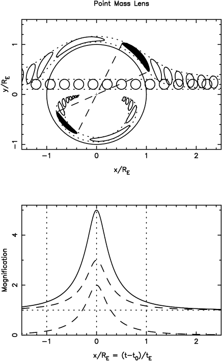
Figure 1: Top panel shows snapshots of the unlensed background star and of the two distorted images of it that appear on opposite sides of the lens during a micro-lensing event. The major image passes over the top of the Einstein ring, while the minor image executes a loop inside the Einstein ring. The two images become compressed in radius but elongated in azimuth as they approach the Einstein ring, resulting in a net magnification. This produces the characteristic lensing lightcurves shown in the bottom panel, where dashed lines show the separate lightcurves of the two images, $A_{+}(t)$ and $A_{-}(t)$, and the solid line is their sum, $A(t)$. Note that $A_{+}(t)=1+A_{-}(t)$.

Fig 1 shows the Einstein ring and trajectories of the two images during a microlensing event. On the lens plane perpendicular to the line of sight, we define cartesian coordinates $x$ and $y$ with the origin at the lens star, the source star moving in the $+x$ direction and crossing the $+y$ axis at closest approach. In units of $\theta_{\rm E}$, the source-lens separation is

$$u=\left(u_{0}^{2}+u_{x}^{2}\right)^{1/2}\ ,$$ (8)

with $u_{0}$ the separation at closest approach, and

$$u_{x}=\mbox{$\frac{\displaystyle{\mu\,(t-t_{0})}}{\displaystyle{\theta_{\rm E}}}$}=\mbox{$\frac{\displaystyle{(t-t_{0})}}{\displaystyle{t_{\rm E}}}$}\ ,$$ (9)

where $\mu$ is the relative proper motion, $t_{0}$ is the time of closest approach, and the event timescale,

$$t_{\rm E}=\mbox{$\frac{\displaystyle{\theta_{\rm E}}}{\displaystyle{\mu_{\rm rel}}}$}\ ,$$ (10)

is the time to cross the radius of the Einstein ring.

The image-lens separations satisfy $u_{+}^{2}u_{-}^{2}=1$, so that, as seen in Fig 1, the major image at $u_{+}$ is always outside the Einstein ring, while the minor image at $u_{-}$ remains inside. The major image slides “over the top” of the Einstein ring, while the minor image traces a loop inside the ring. Both images become brighter as they approach the Einstein ring. Each point on the disc of the source star maps to a corresponding lensed position on the image. The images are thus stretched in azimuth by a factor $u_{\pm}/u$ and squashed in radius by ${\rm d}u_{\pm}/{\rm d}u$. With surface brightness conserved, the net magnification arising from the increased solid angle is

$$\begin{array}[]{rl}A_{\pm}&=\left|\mbox{$\frac{\displaystyle{u_{\pm}}}{\displaystyle{u}}$}\right|\left|\mbox{$\frac{\displaystyle{{\rm d}u_{\pm}}}{\displaystyle{{\rm d}u}}$}\right|=\mbox{$\frac{\displaystyle{1}}{\displaystyle{2u}}$}\mbox{$\frac{\displaystyle{{\rm d}}}{\displaystyle{{\rm d}u}}$}\left[u_{\pm}^{2}\right]\\ &=\mbox{$\frac{\displaystyle{u_{\pm}^{2}}}{\displaystyle{u_{+}^{2}-u_{-}^{2}}}$}=\mbox{$\frac{\displaystyle{T\pm B}}{\displaystyle{2B}}$}=\mbox{$\frac{\displaystyle{A\pm 1}}{\displaystyle{2}}$}\ .\end{array}$$ (11)

The image magnifications satisfy $A_{+}=1+A_{-}$, and the total magnification is

$$A\equiv A_{+}+A_{-}=\mbox{$\frac{\displaystyle{u_{+}^{2}+u_{-}^{2}}}{\displaystyle{u_{+}^{2}-u_{-}^{2}}}$}=\mbox{$\frac{\displaystyle{T}}{\displaystyle{B}}$}=\mbox{$\frac{\displaystyle{u^{2}+2}}{\displaystyle{u\left(u^{2}+4\right)^{1/2}}}$}\ .$$ (12)

Since $u$ changes with time, this defines a characteristic point-source point-lens (PSPL) lightcurve (Fig 1). Power-law approximations (Fig. 2) for large, intermediate, and small $u$ are

$$A(u)-1=\left\{\begin{array}[]{cl}2u^{-4}&u\stackrel{{\scriptstyle>}}{{{}_{\sim}}}2.5\ ,\\ u^{-2}/3&0.3\stackrel{{\scriptstyle<}}{{{}_{\sim}}}u\stackrel{{\scriptstyle<}}{{{}_{\sim}}}2.5\ ,\\ u^{-1}&u\stackrel{{\scriptstyle<}}{{{}_{\sim}}}0.3\ .\end{array}\right.$$ (13)

Note that $A(u)$ has the inverse:

$$u=\left(2\left[\left(1-A^{-2}\right)^{-1/2}-1\right]\right)^{1/2}\ .$$ (14)

Figure 2: The point-source point-lens (PSPL) magnification $A(u)$ compared with the power-law approximations defined in Eqn 13.

2.2 Finite Source Size

For a point source at high magnification, as $u\rightarrow 0$, $A\rightarrow 1/u$ becomes formally infinite, corresponding to the formation of an Einstein ring of infinite magnification and infitesimal thickness. This point-source approximation breaks down, however, when the source star’s finite size becomes important. In Fig.1, curvature of the highly magnified images is already evident. At still higher magnifications, the major and minor images extend farther in azimuth, eventually touching each other and merging to form an Einstein ring of finite width. The magnification remains finite due to the finite source size [Bennett & Rhie 1996, Dominik 1998]. The source star’s angular radius $\theta_{\rm S}=R_{\rm S}/D_{\rm S}$ becomes comparable to the angular radius $\theta_{\rm E}$ of the Einstein ring, at

$$\begin{array}[]{rl}u_{\rm S}&\equiv\mbox{$\frac{\displaystyle{\theta_{\rm S}}}{\displaystyle{\theta_{\rm E}}}$}=\mbox{$\frac{\displaystyle{R_{\rm S}}}{\displaystyle{\left(2\,S_{\rm L}\,D_{\rm S}\,X\left(1-X\right)\right)^{1/2}}}$}\\ \\ &=0.0013\left(\mbox{$\frac{\displaystyle{R_{\rm S}}}{\displaystyle{R_{\odot}}}$}\right)\left(\mbox{$\frac{\displaystyle{M_{L}}}{\displaystyle{M_{\odot}}}$}\right)^{-1/2}\left(\mbox{$\frac{\displaystyle{X}}{\displaystyle{1-X}}$}\right)^{1/2}\ .\end{array}$$ (15)

Finite-source effects set in at high magnification, $A\stackrel{{\scriptstyle>}}{{{}_{\sim}}}1/u_{\rm S}$, thus (for $M_{\rm L}\sim 0.3\,M_{\odot}$) at $A\stackrel{{\scriptstyle>}}{{{}_{\sim}}}500$ for a main-sequence source star with $R_{\rm S}\sim R_{\odot}$, or already at $A\stackrel{{\scriptstyle>}}{{{}_{\sim}}}5$ for a giant source star with $R_{\rm S}\sim 100\,R_{\odot}$.

Finite source effects are important for planet anomalies when the source star’s angular radius $\theta_{\rm S}$ exceeds that of the planet’s Einstein ring [Bennett & Rhie 1996]. Since $\theta_{\rm p}=q^{1/2}\,\theta_{\rm E}$, the finite source effect is important when

$$q\stackrel{{\scriptstyle<}}{{{}_{\sim}}}\left(\mbox{$\frac{\displaystyle{\theta_{\rm S}}}{\displaystyle{\theta_{\rm E}}}$}\right)^{2}\sim 2\times 10^{-6}\left(\mbox{$\frac{\displaystyle{R_{\rm S}}}{\displaystyle{R_{\odot}}}$}\right)^{2}\left(\mbox{$\frac{\displaystyle{M_{L}}}{\displaystyle{M_{\odot}}}$}\right)^{-1}\left(\mbox{$\frac{\displaystyle{X}}{\displaystyle{1-X}}$}\right)\ .$$ (16)

Since $m_{\oplus}=3\times 10^{-6}M_{\odot}$, this is

$$m_{\rm p}=q\,M_{\rm L}\stackrel{{\scriptstyle<}}{{{}_{\sim}}}0.6\,m_{\oplus}\left(\mbox{$\frac{\displaystyle{R_{\rm S}}}{\displaystyle{R_{\odot}}}$}\right)^{2}\left(\mbox{$\frac{\displaystyle{X}}{\displaystyle{1-X}}$}\right)\ .$$ (17)

For large source stars the anomaly from a small planet can be smeared out and diluted in amplitude, rendering it undetectable. On this basis, detection of Earth-mass planets is more favourable with main sequence source stars [Bennett & Rhie 1996], though a detectable ($\sim 5$%) signal can arise even when the source star is a giant [Dominik, et al. 2007], provided the planet’s alignment with one of the image trajectories is favourable. We do not consider finite-source effects further in this paper.

2.3 Binary Lens Anomalies

A planet near the lens star acts like a small defect in the gravitational lens. If the planet is well away from the two image trajectories, the light it deflects does not reach Earth. In this case the planet has no measurable effect on the lightcurve and thereby evades detection. However, if the planet is close to one of the image trajectories, its gravity can significantly perturb the bundle of light rays that would otherwise reach Earth. This distorts the image and changes the magnification to produce a brief anomaly in the lightcurve. The magnification curve $A_{2}(t)$ for a star+planet lens deviates by a factor $1+\delta(t)$ from the corresponding PSPL magnification curve $A_{1}(t)$:

$$A_{2}(t)=A_{1}(t)\left(1+\delta(t)\right)\ .$$ (18)

This defines the planet anomaly $\delta(t)$, which depends on three additional parameters: the mass ratio $q$, and the coordinates, $x$ and $y$, of the planet’s projected position on the lens plane.

The planet anomaly may be brief but large. The planet’s Einstein ring radius is

$$r_{\rm p}\equiv R_{\rm E}\,q^{1/2}\ .$$ (19)

The planet anomaly may be large when one of the source images passes closer to the planet than $r_{\rm p}$, provided the source is not much larger than $r_{\rm p}$. The duration of the planet anomaly is roughly the time it takes the image to cross the diameter of the planet’s Einstein ring,

$$t_{\rm p}\equiv t_{\rm E}\,q^{1/2}\ .$$ (20)

Detecting the planet requires data points in the lightcurve of sufficient accuracy and at the right time to detect the anomaly produced as the image passes by the planet.

3 Planet Detection Zones

3.1 Definition of Detection Zone

We define the “detection zone” as the region on the lens plane ($x$,$y$) where the lightcurve anomaly $\delta(t,x,y,q)$ is large enough to be detected or ruled out with high confidence by the observations. For $N$ data points with fractional accuracy $\sigma_{i}$ at times $t_{i}$, the detection zone is defined by

$$\sum_{i=1}^{N}\left(\mbox{$\frac{\displaystyle{\delta(t_{i},x,y,q)}}{\displaystyle{\sigma_{i}}}$}\right)^{2}>\Delta\chi^{2}\ ,$$ (21)

for some detection threshold $\Delta\chi^{2}$. This detection threshold must be set high enough so that noise affecting the observations does not produce false triggers at an unacceptably high rate. $\Delta\chi^{2}$ in the range 25 to 100 corresponds to a $5\sigma$ to $10\sigma$ deflection in the lightcurve if the anomaly is confined to a single data point.

Fig. 3 highlights the detection zones for a planet with mass ratio $q=10^{-3}$ derived from a lightcurve $A(t)$ with maximum magnification $A_{0}=5$. Data points uniformly spaced in time sample the lightcurve with an accuracy $\sigma=(5/A^{1/2})$%, and the detection criterion is $\Delta\chi^{2}>25$. Each data point probes for planets close to the corresponding major and minor image positions. If a planet is placed inside one of these detection zones, the lightcurve at time $t_{i}$ is perturbed by $\delta>5\,\sigma=(25/A^{1/2})\%$. Improving the accuracy of the data or increasing the mass of the planet enlarges the size of the detection zone.

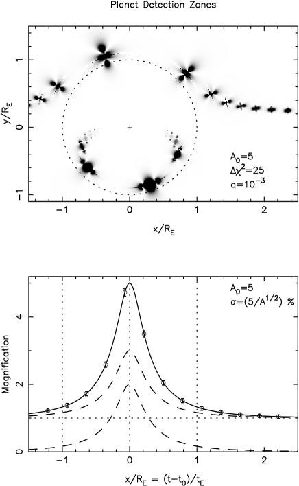
Figure 3: Detection zones on the lens plane indicate the regions where a planet with mass ratio $q=m/M=10^{-3}$ is detected with $\Delta\chi^{2}>25$. The lightcurve $A(t)$ has maximum magnification $A_{0}=5$, and the accuracy of the measurements is $\sigma=(5/A^{1/2})$%. Each data point probes for planets close to the two images of the background star. The detection zone areas scale roughly as $\Omega\approx R_{\rm E}^{2}\,(2\,A-1)\,q\,/(\sigma\,\Delta\chi)$.

3.2 Numerical Evaluation of Detection Zone Areas

If the data points in the lightcurve are widely spaced, as they are in Fig. 3, then the detection zones arising from different data points are well isolated from each other. We may then evaluate numerically the area $\Omega$ of the detection zone that is carved out by each data point. This quantifies the planet discovery potential of each data point.

Fig. 4 shows a close-up of the detection zones defined by this criterion. The region displayed is chosen in advance from rough estimates and is used for numerical evaluation of the dectection zone area $\Omega$. The cases shown illustrate how the detection zones shrink and change shape as the magnification $A(u)$ declines with increasing lens-source separation $u$. The detection zone shapes are complicated. At small $u$ and high $A$ they bear some resemblance to 4-leafed clovers with radial and azimuthal lobes straddling the image positions. With increasing $u$, decreasing $A$, the azimuthal lobes of the major image detection zone collapse radially. The radial lobes then merge radially to form a circular detection zone as $u\rightarrow\infty$. On the minor image detection zone, the radial lobes merge and vanish, leaving two isolated azimuthal lobes that shrink and vanish.

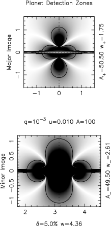
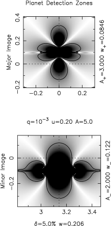
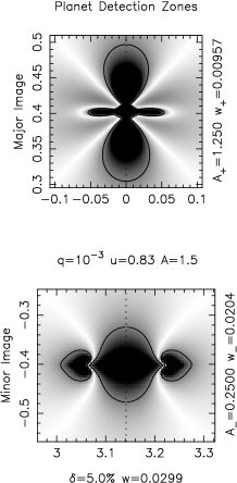
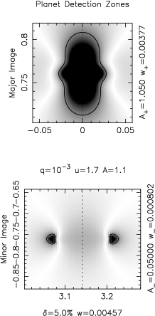
Figure 4: Planet detection zones for mass ration $q=10^{-3}$ near the major and minor image positions for data points at magnifications $A=100$, 5, 1.5, and 1.1. The detection zones are symmetric around the image positions in ($\theta$,$\ln{u})$ coordinates. For $u\rightarrow\infty$ and $A\rightarrow 1$ the major image detection zone becomes circular and the minor image detection zone splits in two and vanishes.

3.3 Scaling Laws for Detection Zone Areas

It will be helpful to understand how planet detection zone areas scale with the accuracy of the data, the source magnification, and the mass of the planet. If accurate scaling laws can be found, we may then avoid long numerical calculations to determine the detection zone area. In this section we develop a useful analytic formula, and test it against detailed numerical integrations.

Consider first a planet located quite far from the lens star, affecting the major image at a time well before or well after the stellar lensing event, when $u_{+}>>1$ and $A_{+}\approx 1$. In this case the planet and star act as independent lenses, and a significant anomaly occurs when the major image sweeps past the position of the planet. If $z$ is the separation between the planet and the major image, the planet magnifies the major image by a factor $A(u_{\rm p})$, where $u_{\rm p}=z/r_{\rm p}$, and $r_{\rm p}=q^{1/2}\,R_{\rm E}$ is the planet’s Einstein ring radius.

A data point with fractional uncertainty $\sigma$ can detect the anomaly $\delta$ when

$$\delta=A(u_{\rm p})-1>\sigma\left(\Delta\chi^{2}\right)^{1/2}\ .$$ (22)

This criterion corresponds to a circular detection zone around the major image at the time of the observation. The radius of the detection zone is found by solving Eqn. (22) for $u_{\rm p}$ and hence $z=r_{\rm p}u_{\rm p}$. Using Eqn. (14) to invert $A(u_{\rm p})$, the area of the detection zone is

$$\mbox{$\frac{\displaystyle{\Omega}}{\displaystyle{\pi r_{\rm p}^{2}}}$}=\left(\mbox{$\frac{\displaystyle{z}}{\displaystyle{r_{\rm p}}}$}\right)^{2}=\left[2\left(1-\left(1+\delta\right)^{-2}\right)^{-1/2}-1\right]\ .$$ (23)

Using the approximations in Eqn. (13), the corresponding approximations for the detection zone area are

$$\mbox{$\frac{\displaystyle{\Omega}}{\displaystyle{\pi r_{\rm p}^{2}}}$}=\left\{\begin{array}[]{cl}\left(2/\delta\right)^{1/2}&\delta\stackrel{{\scriptstyle<}}{{{}_{\sim}}}0.05\ ,\\ \left(3\ \delta\right)^{-1}&0.05\stackrel{{\scriptstyle<}}{{{}_{\sim}}}\delta\stackrel{{\scriptstyle<}}{{{}_{\sim}}}3\ ,\\ \delta^{-2}&\delta\stackrel{{\scriptstyle>}}{{{}_{\sim}}}3\ .\end{array}\right.$$ (24)

Fig. 5 indicates that the middle approximation predicts fairly accurately the detection zone area for anomalies in the range $0.05<\delta<3$. For $\Delta\chi^{2}=25$ this range corresponds to fractional uncertainties $0.01<\sigma<0.6$, quite appropriate for CCD data, giving

$$\mbox{$\frac{\displaystyle{\Omega}}{\displaystyle{R_{E}^{2}}}$}=\mbox{$\frac{\displaystyle{\pi\,q}}{\displaystyle{3\,\delta}}$}\ .$$ (25)

Figure 5: The detection zone area $\Omega$ scales with the area $\pi r_{\rm p}^{2}$ of the planet’s Einstein ring, and decreases with the size of the lightcurve anomaly $\delta$ that can be detected by the data. The approximations (dashed lines) are those defined in Eqn. 24.

Now move the planet closer to the lens star. The planet acts as a defect in the stellar lens, and the resulting detection zone can have a quite complicated shape (Fig. 4). We guess that the detection zone area may scale roughly with the magnification $A$. However, we find that $\Omega\propto 2A-1$ is a better approximation:

$$\mbox{$\frac{\displaystyle{\Omega}}{\displaystyle{R_{\rm E}^{2}}}$}\approx\mbox{$\frac{\displaystyle{\pi\,q}}{\displaystyle{3\,\delta}}$}\left(2\,A-1\right)\ .$$ (26)

Fig. 4 shows that the detection zones are roughly symmetric as a function of $\ln{u}$ and $\theta$ rather than $x$ and $y$. It may therefore be more appropriate to express detection zone areas using a ${\rm d}\theta\,{\rm d}\ln{u}$ metric, evaluating

$$w=\int P({\rm det}|u,\theta)\ \mbox{$\frac{\displaystyle{{\rm d}u\ {\rm d}\theta}}{\displaystyle{u}}$}\ ,$$ (27)

rather than

$$\mbox{$\frac{\displaystyle{\Omega}}{\displaystyle{R_{\rm E}^{2}}}$}=\int P({\rm det}|u,\theta)\ u\,{\rm d}u\,{\rm d}\theta=\int P({\rm det}|x,y)\ {\rm d}x\,{\rm d}y\ .$$ (28)

The ${\rm d}\theta\,{\rm d}\ln{u}$ metric may be appropriate from a second perspective. Exo-planet orbits should have random orientations, so the planets should be uniformly distributed in $\theta$. If their orbit size distribution is also roughly uniform in $\log{a}$, then the planet distribution on the lens plane will be roughly uniform in $\ln{u}$, and the planet detection probability will decline to zero long after the peak of an event, rather than reaching a positive asymptotic value. In effect the ${\rm d}\theta\,{\rm d}\ln{u}$ metric recognizes a detection zone with area $\Omega$ as more likely to include a planet, and therefore more valuable to us, when it is measured at small $u$ and probes a larger range of $\log{u}$.

For small detection zones the two metrics are related by

$$w\approx\mbox{$\frac{\displaystyle{\Omega}}{\displaystyle{R_{\rm E}^{2}\,u^{2}}}$}\approx\mbox{$\frac{\displaystyle{\pi\,q}}{\displaystyle{3\,\delta}}$}\left(\mbox{$\frac{\displaystyle{2A-1}}{\displaystyle{u^{2}}}$}\right)\ .$$ (29)

But we must be more careful to treat separately the major and minor image detection zones, surrounding the images at $u_{+}$ and $u_{-}$ respectively. This gives

$$w_{\pm}\approx\mbox{$\frac{\displaystyle{\pi\,q}}{\displaystyle{3\,\delta}}$}\ F_{\pm}(A)\ ,$$ (30)

where for the major image at $u_{+}$

$$F_{+}(A)\equiv\mbox{$\frac{\displaystyle{2\,A_{+}-1}}{\displaystyle{\left(u_{+}\right)^{2}}}$}=\mbox{$\frac{\displaystyle{2\,T}}{\displaystyle{B\left(T+B\right)}}$}=A\,\left(\mbox{$\frac{\displaystyle{A-1}}{\displaystyle{A+1}}$}\right)^{1/2}\ ,$$ (31)

and for the minor image at $u_{-}$

$$F_{-}(A)\equiv\mbox{$\frac{\displaystyle{2\,A_{-}}}{\displaystyle{\left(u_{-}\right)^{2}}}$}=\mbox{$\frac{\displaystyle{2}}{\displaystyle{B}}$}=\left(A+1\right)\,\left(\mbox{$\frac{\displaystyle{A-1}}{\displaystyle{A+1}}$}\right)^{1/2}\ .$$ (32)

In deriving the above expressions, we used Eqns. (7), (11) and (12) to write

$$\begin{array}[]{rl}A_{\pm}=&\mbox{$\frac{\displaystyle{T\pm B}}{\displaystyle{2\,B}}$}\ ,\hskip 8.53581pt\left(u_{\pm}\right)^{2}=\mbox{$\frac{\displaystyle{T\pm B}}{\displaystyle{2}}$}\ ,\\ \\ T=&u_{+}^{2}+u_{-}^{2}=u^{2}+2=\mbox{$\frac{\displaystyle{2\,A}}{\displaystyle{\left(A^{2}-1\right)^{1/2}}}$}\ ,\\ \\ B=&u_{+}^{2}-u_{-}^{2}=u\,\left(u^{2}+4\right)^{1/2}=\mbox{$\frac{\displaystyle{2}}{\displaystyle{\left(A^{2}-1\right)^{1/2}}}$}\ .\end{array}$$ (33)

The total detection zone area, summing the detection areas of both images, is

$$w=\mbox{$\frac{\displaystyle{\pi\,q}}{\displaystyle{3\,\delta}}$}F(A)=\mbox{$\frac{\displaystyle{\pi\,q\,F(A)}}{\displaystyle{3\,\left(\Delta\chi^{2}\right)^{1/2}\,\sigma(\ln{A})}}$}\ ,$$ (34)

with $\sigma(\ln{A})$ the fractional accuracy in measuring $A$, $\Delta\chi^{2}$ the threshold for planet detection, and

$$\begin{array}[]{rl}F(A)&\equiv F_{+}(A)+F_{-}(A)\\ \\ &=\mbox{$\frac{\displaystyle{2}}{\displaystyle{B}}$}\,\left(\mbox{$\frac{\displaystyle{2\,T+B}}{\displaystyle{T+B}}$}\right)=\left(2\,A+1\right)\left(\mbox{$\frac{\displaystyle{A-1}}{\displaystyle{A+1}}$}\right)^{1/2}\ .\end{array}$$ (35)

The functions $F_{\pm}(A)$, for the separate images and $F(A)$ for the total detection zone area are plotted in Fig. 6 for an event with $A_{0}=5$.

Figure 6: The magnification, detection zone area, image velocity, and detection zone crossing time are shown for an event with peak magnification $A_{0}=5$. The dashed and dash-dot curves are for the major and minor images respectively, except for the image velocity panel where the dashed curve is ${\rm d}\theta/{\rm d}t$ while the dash-dot curve is ${\rm d}\ln{u}/{\rm d}t$ for the major image.

3.4 Analytic vs Numerical Detection Zone Areas

Figure 7: The detection zone areas $w$ in the ${\rm d}\theta\,{\rm d}\ln{u}$ metric increase with magnification $A$, increase with mass ratio $q$, and decrease with the size of the lightcurve anomaly $\delta$ that can be detected by the data. The fast analytic approximation (dotted) defined in Eqn. (34) is compared with more exact numerical integrations. Dotted curves in the lower panel give fractional contributions of the major and minor images, in the analytic approximation.

Fig. 7 compares numerically-integrated detection zone areas with the analytic result in Eqn. (34). The figure shows how $w$ depends on $A-1$ for three mass ratios, $q=10^{-3}$, $10^{-4}$ and $10^{-5}$, and for three accuracies, $\delta=\sigma(\ln{A})\left(\Delta\chi^{2}\right)^{1/2}=5$, 10 and 20%.

The analytic approximation clearly captures the main scaling, $w\propto q\,A/\delta$, for $2<A<300$. However, it is a rough guide rather than a superb approximation. At moderately high magnifications, $10<A<300$, the analytic and numerical results agree to within $\sim 5$%. Here we have $F_{+}\approx\,F_{-}\approx(2\,A-1)/2$, the two images contributing roughly equally. At intermediate magnifications, $2<A<10$, the analytic result is low by up to $\sim 10$%. This $A$-dependent bias could be reduced by adjusting the formula for $F(A)$ in Eqn. (35). However, the accuracy is already sufficient for our purposes in the range $2<A<300$. We discuss below the breakdown at larger and smller magnifications.

At very high magnifications, $A>300$, our analytic approximation breaks down because the detection zones extend so far in azimuth that the major and minor image zones touch each other and merge together. Since the detection zones span a roughly equal range in $\theta$ and in $\ln{u}$, the saturation in $\theta$ should set in when $w\sim\left(2\,\pi\,q\,A/3\,\delta\right)\stackrel{{\scriptstyle>}}{{{}_{\sim}}}\pi^{2}$, i.e.

$$A\stackrel{{\scriptstyle>}}{{{}_{\sim}}}\mbox{$\frac{\displaystyle{3\,\pi}}{\displaystyle{2}}$}\,\mbox{$\frac{\displaystyle{\delta}}{\displaystyle{q}}$}\ .$$ (36)

We enter a new regime in which the azimuthally-merged detection zone may continue to expand in $\ln{u}$ but is saturated in $\theta$. The slope should drop to $w\propto\left(q\,A/\delta\right)^{1/2}$, i.e.

$$w\left(A\stackrel{{\scriptstyle>}}{{{}_{\sim}}}\mbox{$\frac{\displaystyle{\delta}}{\displaystyle{q}}$}\right)\approx 2\,\pi\left(\mbox{$\frac{\displaystyle{2\,\pi\,q\,A}}{\displaystyle{3\,\delta}}$}\right)^{1/2}\ .$$ (37)

These expectation are roughly consistent with the behaviour in Fig. 7.

Note that in the very-high magnification regime finite source effects will also become important, altering the relationship between $u$ and $A$ with $u>u_{\rm S}$, as discussed in Sec. 2.2. As we neglect both effects in our analysis, our scaling law applies only up to a maximum magnification $A\stackrel{{\scriptstyle<}}{{{}_{\sim}}}\delta/q\sim 300$.

At low-ish magnifications, $A<2$, Fig. 7 shows that the analytic formula over-predicts detection zone areas by factors of up to $\sim 3$. The structure is independent of $q$ but depends on $\delta$ and $A$, due to the complicated structure of the detection zones as seen in Fig. 4. In this regime, $A\approx 1-2\,u^{-4}$, $F_{+}\approx u^{-2}$, $F_{-}\approx 2\,u^{-2}$, and $F\approx 3\,u^{-2}$. With $F_{-}\approx 2\,F_{+}$, the analytic formula gives the minor image twice the detection area of the major image. The $F_{+}$ formula has correct asymptotic behaviour at both high and low magnifications, so the problem is with the $F_{-}$ formula. In fact at low magnifications the radial lobes of the minor image merge and disappear, as seen in the right two columns of Fig. 4. This cuts the total detection zone area by a factor of about 3 when $A$ drops below a threshold,

$$A-1\approx\mbox{$\frac{\displaystyle{2}}{\displaystyle{u^{4}}}$}\stackrel{{\scriptstyle<}}{{{}_{\sim}}}3\,\delta\ .$$ (38)

As shown in Fig. 8, a fairly successful attempt to repair this deficit is

$$w=\mbox{$\frac{\displaystyle{\pi\,q}}{\displaystyle{3\,\delta}}$}\left(\mbox{$\frac{\displaystyle{A-1}}{\displaystyle{A+1}}$}\right)^{1/2}\left(A+\left(1+A\right)\,C\left(x\right)\right)\ ,$$ (39)

where $x\approx 3\,\delta/(A-1)\approx 3\,u^{4}\,\delta/2$, and

$$C(x)\approx max\left[0,\mbox{$\frac{\displaystyle{1-x^{2}}}{\displaystyle{1+x^{2}}}$}\right]$$ (40)

cuts off the minor image contribution at the appropriate threshold. However, this makes $F_{-}$ depend on $\delta$ as well as $A$.

Figure 8: As in Fig. 7 but using the approximation in defined in Eqn. (39) rather than Eqn. (34).

3.5 Detection Zone Crossing Timescale

The cadence of observations aiming to detect planet-like anomalies should ideally be matched to the time it takes for the images to cross the detection zones, so that each measurement probes for planets in an independent region of the lens plane, rather than overlapping with the region already sampled by previous measurements. This will clearly depend on the size of the detection zones, and on the speed at which the images move on the lens plane.

If we approximate the width of the detection zone as the square root of its area, then the detection zone crossing timescale is

$$t_{\pm}\approx\left(\mbox{$\frac{\displaystyle{w_{\pm}}}{\displaystyle{v^{2}}}$}\right)^{1/2}\approx\left(\mbox{$\frac{\displaystyle{q\,F_{\pm}(A)}}{\displaystyle{\delta\,v^{2}}}$}\right)^{1/2}\ ,$$ (41)

where $w_{\pm}=q\,F_{\pm}(A)/\delta$ is the detection zone area in the ${\rm d}\theta\,{\rm d}\ln{u}$ metric, and $v$ is the corresponding image speed,

$$v^{2}=\left(\mbox{$\frac{\displaystyle{{\rm d}\theta}}{\displaystyle{{\rm d}t}}$}\right)^{2}+\left(\mbox{$\frac{\displaystyle{{\rm d}\ln{u_{\pm}}}}{\displaystyle{{\rm d}t}}$}\right)^{2}=\dot{\theta}^{2}+\left(\mbox{$\frac{\displaystyle{\dot{u}_{\pm}}}{\displaystyle{u_{\pm}}}$}\right)^{2}\ .$$ (42)

We show below that $v$ is actually the same for both images, they move at the same speed on the $\theta$ vs $\ln{u}$ plane. The image speed and planet detection timescale are plotted in Fig. 6 for an event with $A_{0}=5$.

To evaluate the azimuthal velocity $\dot{\theta}$, note that both images sweep around in $\theta$ at the same rate as the unlensed source position. With $x=(t-t_{0})/t_{E}$ and $y=u_{0}$, the unlensed source position moves with

$$\dot{x}=\mbox{$\frac{\displaystyle{1}}{\displaystyle{t_{E}}}$}\ ,\hskip 14.22636pt\dot{y}=0\ .$$ (43)

Differentiate $\theta=\arctan{\mbox{$\frac{\displaystyle{y}}{\displaystyle{x}}$}}$ to find

$$\dot{\theta}=\dot{x}\,\mbox{$\frac{\displaystyle{{\rm d}\theta}}{\displaystyle{{\rm d}x}}$}=\mbox{$\frac{\displaystyle{-\dot{x}\,y}}{\displaystyle{x^{2}+y^{2}}}$}=\mbox{$\frac{\displaystyle{-u_{0}}}{\displaystyle{u^{2}\,t_{E}}}$}\ .$$ (44)

Evaluating the $\ln{u_{\pm}}$ image velocities is more involved, but leads to a simple result. First, differentiate $u^{2}=x^{2}+y^{2}$ to find

$$\dot{u}=\dot{x}\,\mbox{$\frac{\displaystyle{{\rm d}u}}{\displaystyle{{\rm d}x}}$}=\mbox{$\frac{\displaystyle{\dot{x}\,x}}{\displaystyle{u}}$}=\mbox{$\frac{\displaystyle{x}}{\displaystyle{u\,t_{E}}}$}\ .$$ (45)

Next, differentiate $\left(u_{\pm}\right)^{2}=\left(T\pm B\right)/2$ to find

$$\mbox{$\frac{\displaystyle{\dot{u}_{\pm}}}{\displaystyle{u_{\pm}}}$}=\mbox{$\frac{\displaystyle{\dot{T}\pm\dot{B}}}{\displaystyle{4\left(u_{\pm}\right)^{2}}}$}=\mbox{$\frac{\displaystyle{u\,\dot{u}\,\left(1\pm A\right)}}{\displaystyle{2\left(u_{\pm}\right)^{2}}}$}\ ,$$ (46)

where we have differentiated Eqn. (33) to find

$$\dot{T}=2\,u\,\dot{u}\ ,\hskip 8.53581pt\dot{B}=2\,u\,\dot{u}\,A\ .$$ (47)

Then, since $A=T/B$, and $\left(u_{\pm}\right)^{2}=\left(T\pm B\right)/2$,

$$\mbox{$\frac{\displaystyle{\dot{u}_{\pm}}}{\displaystyle{u_{\pm}}}$}=\mbox{$\frac{\displaystyle{u\,\dot{u}\,\left(B\pm T\right)}}{\displaystyle{B\,\left(T\pm B\right)}}$}=-\mbox{$\frac{\displaystyle{u\,\dot{u}}}{\displaystyle{B}}$}=-\mbox{$\frac{\displaystyle{x}}{\displaystyle{t_{E}\,B}}$}\ .$$ (48)

Notice that both images have the same velocity in $\ln{u}$, as well as in $\theta$, so that the image velocity $v$ is the same for both images.

Substituting Eqns. (48) and (44) into (42), the image speed on the $\theta,\ln{u}$ plane is

$$\left(v\,t_{E}\right)^{2}=\mbox{$\frac{\displaystyle{u_{0}^{2}}}{\displaystyle{u^{4}}}$}+\mbox{$\frac{\displaystyle{x^{2}}}{\displaystyle{B^{2}}}$}=\mbox{$\frac{\displaystyle{1+4\,u_{0}^{2}/u^{4}}}{\displaystyle{u^{2}+4}}$}=\mbox{$\frac{\displaystyle{u^{4}+4\,u_{0}^{2}}}{\displaystyle{u^{4}\left(u^{2}+4\right)}}$}\ .$$ (49)

The image speed is plotted in Fig. 6 for an event with $A_{0}=5$. The azimuthal velocity $\dot{\theta}$ dominates near the peak, and the radial velocity ${\rm d}\ln{u}/{\rm d}t$ dominates in the wings of the lightcurve. For large $u^{2}$, the image speed varies as $v\,t_{\rm E}\approx 1/u$. The maximum speed $v_{0}\,t_{\rm E}=1/u_{0}$ is reached at the peak of the event, at $t=t_{0}$, where $u=u_{0}$.

The planet anomaly crossing timescale is given by

$$\left(\mbox{$\frac{\displaystyle{t_{\pm}}}{\displaystyle{t_{E}}}$}\right)^{2}=\mbox{$\frac{\displaystyle{w_{\pm}}}{\displaystyle{\left(v\,t_{E}\right)^{2}}}$}=\mbox{$\frac{\displaystyle{q\,F_{\pm}(A)}}{\displaystyle{\delta}}$}\mbox{$\frac{\displaystyle{u^{2}+4}}{\displaystyle{1+4\,u_{0}^{2}/u^{4}}}$}\ .$$ (50)

Crossing times for the major and minor images are shown in the lower panel of Fig. 6. The crossing time is slightly larger for the minor image, by a factor $\left(F_{-}/F_{+}\right)^{1/2}=\left(\left(A+1\right)/A\right)^{1/2}$ (see Eqns. (31) and (32)). The crossing time at first rises due to the increasing size of the detection zone, and then drops to a minimum at the peak, where the maximum image velocity $v_{0}=1/\left(t_{\rm E}\,u_{0}\right)$ is reached. This minimum crossing time, at the peak of the event, is

$$\begin{array}[]{rl}t_{\pm}(0)&=t_{\rm E}\,u_{0}\,\left(\mbox{$\frac{\displaystyle{q}}{\displaystyle{\delta}}$}\left(A_{0}+\mbox{$\frac{\displaystyle{1}}{\displaystyle{2}}$}\mp\mbox{$\frac{\displaystyle{1}}{\displaystyle{2}}$}\right)\right)^{1/2}\left(\mbox{$\frac{\displaystyle{A_{0}-1}}{\displaystyle{A_{0}+1}}$}\right)^{1/4}\\ \\ &\approx t_{\rm E}\,\left(\mbox{$\frac{\displaystyle{q}}{\displaystyle{\delta\,A_{0}}}$}\right)^{1/2}\ .\end{array}$$ (51)

Here the final approximation, using $F_{\pm}\approx A$ and $u\approx A^{-1}$, holds to 15% or better for $A_{0}\stackrel{{\scriptstyle>}}{{{}_{\sim}}}3$.

For a specific example, consider the crossing time for a Jupiter-like planet with $q=10^{-3}$, in a typical event with $t_{\rm E}=30$ d. For a peak magnification $A_{0}=5$, as in Fig. 6, we have $u_{0}=0.2$, $F_{+}=5\,\left(4/6\right)^{1/2}=4.1$ and $F_{-}=6\,\left(4/6\right)^{1/2}=4.9$. For a good data point with $\sigma\left(\ln{A}\right)=1$%, and a detection threshold at $\Delta\chi^{2}=100$, the smallest detectable planet-like anomaly deviates by $\delta=\sigma(\ln{A})\,\left(\Delta\chi^{2}\right)^{1/2}=0.1$. The crossing time for the major image is

$$t_{+}(0)=30\times 0.2\,\left(\mbox{$\frac{\displaystyle{0.001}}{\displaystyle{0.1}}$}5\right)^{1/2}\left(\mbox{$\frac{\displaystyle{4}}{\displaystyle{6}}$}\right)^{1/4}=1.2~{}{\rm d}\ .$$ (52)

For an Earth-mass planet and a typical lens mass $M_{\rm L}\approx 0.3~{}M_{\odot}$ the mass ratio is $q=10^{-5}$, and the crossing time is

$$t_{\pm}(0)\approx 2.3~{}h\left(\mbox{$\frac{\displaystyle{t_{\rm E}}}{\displaystyle{30~{}{\rm d}}}$}\right)\left(\mbox{$\frac{\displaystyle{q}}{\displaystyle{10^{-5}}}$}\right)^{1/2}\left(\mbox{$\frac{\displaystyle{\delta}}{\displaystyle{0.1}}$}\right)^{-1/2}\left(\mbox{$\frac{\displaystyle{A}}{\displaystyle{10}}$}\right)^{-1/2}\ .$$ (53)

4 Optimizing a Microlens Planet Search

4.1 The Observer’s Dilemma

In this section we consider how an observer might try to optimize a microlens planet search. We assume that the observer has many targets to choose from. This is a good assumption because MOA II and OGLE III are finding $\sim 600-1000$ events each year. The observing time available on each night during the winter months when the Galactic Bulge is visible from a southern hemisphere site is of order 10 hours. A dedicated agile telescope spending 2 minutes per target could in principle visit over 100 targets per night. However, why should equal time be devoted to all targets? Surely the brighter and higher-magnification targets warrant more attention. By skipping fainter and/or weakly magnified sources, we can spend more time on the more favourable ones. The resulting planet detection zones, accumulated over all targets during the night, will then be larger, increasing the chances of discovering a planet. At the other extreme, when one source is very highly magnified, should we attend exclusively to that source, and skip all the others, or should we reserve some time for a few of the other sources as well? This is the microlens observer’s perpetual dilemma. The solution we propose is to observe always in a way that aims to maximise the probability of planet discovery.

4.2 Accuracy of Photometry

Because detection zone areas scale as $w\propto\sigma^{-1}$, e.g.  Eqn. (34), a critical issue is the accuracy of photometric measurements that can be achieved, and the rate at which that accuracy improves with exposure time. We assume that the data analysis is close to optimal, so that photon counting statistics dominate the noise budget. Thus CCD readout noise, cosmic ray hits, and other noise sources are neglected in comparison with the Poisson noise from detected star and sky photons. The signal-to-noise ratio then increases as the square-root of the exposure time,

$$\sigma(\ln{A})=\left(\mbox{$\frac{\displaystyle{\tau}}{\displaystyle{\Delta t}}$}\right)^{1/2}\ ,$$ (54)

where $\Delta t$ is the exposure time, and $\tau$ is the exposure time required to reach a signal-to-noise ratio of 1.

The parameter $\tau$ controls the exposure time needed to obtain information on the current magnification $A$. It depends on the telescope collecting area, the detector sensitivity and bandwidth, on the brightness of the magnified source star, and the degree of dilution of its photons by sky background and by other stars that are blended with it. Including these three sources of Poisson noise,

$$\tau=\mbox{$\frac{\displaystyle{f_{\star}+f_{\rm B}+f_{\rm sky}}}{\displaystyle{f_{\star}^{2}}}$}\ ,$$ (55)

where $f_{\star}$, $f_{\rm B}$ and $f_{\rm sky}$ are the number of detected photons per unit time from the magnified source star, from the lens star and other stars blended with the source star, and from the sky, respectively. We elaborate these three Poisson noise sources below.

For a star of magnitude $m_{\star}$ and spectral energy distribution $f_{\lambda}(\lambda)$, we observe thru the atmospere with transmission $T(\lambda)$, with a detector effective area $A_{\rm eff}(\lambda)$. The photon detection rate can be evaluated precisely as

$$f_{\star}=\int\mbox{$\frac{\displaystyle{f_{\lambda}(\lambda)\,{\rm d}\lambda}}{\displaystyle{h\ \nu}}$}A_{\rm eff}(\lambda)\ T(\lambda)\ ,$$ (56)

or approximately as

$$f_{\star}\approx f_{0}(\lambda)\,T(\lambda)\,10^{-0.4m_{\star}}\ .$$ (57)

The photon detection rate from Vega (magnitude 0) is

$$f_{0}(I)\approx 500\,{\rm s}^{-1}\,\left(\mbox{$\frac{\displaystyle{A_{\rm eff}}}{\displaystyle{{\rm cm}^{2}}}$}\right)\left(\mbox{$\frac{\displaystyle{\Delta\lambda}}{\displaystyle{\rm\AA}}$}\right)\ ,$$ (58)

for a telescope with mean effective area $A_{\rm eff}$ over a bandwidth $\Delta\lambda$ near the $I$ band, where most microlens observations are taken (for the $V$ band, Vega’s flux is 1000 rather than 500 photons cm^-2Å^-1s^-1).

For the source star, magnified by a factor $A$,

$$f_{\star}=f_{\rm S}\,A\,T=f_{0}\,T\,10^{-0.4\,m_{\star}}\ .$$ (59)

Stars blended with the magnified source star contribute Poisson noise to the measurement. The source flux $f_{\rm S}$ and blend flux $f_{\rm B}$ are normally measured by fitting observed lightcurves (corrected for atmospheric transmission) with the model

$$f(t)=f_{\rm S}\,A(t)+f_{\rm B}\ .$$ (60)

When using differential flux measurements $\Delta f(t)$, obtained by a difference image analysis, the reference flux added to these is somewhat arbitrary. As a consequence, the blend flux $f_{\rm B}$ arising from the lightcurve fit is also somewhat arbitrary, and can even be negative in some cases.

The blend flux contributing to the Poisson noise includes not only flux from the lens star, and any other stars that are “exactly” coincident on the sky with the magnified source star, but also stars that are close enough on the sky so that the point-spread functions overlap. If $m_{i}$ is the magnitude and $\theta_{i}$ is the angular separation of star $i$ from the target star, the blend flux contributing Poisson noise to the measurement is

$$f_{\rm B}(\Delta)=f_{\star}\sum_{i}10^{-0.4\ \left(m_{i}-m_{\star}\right)}\ e^{-\left(\theta_{i}/\Delta\right)^{2}}\ .$$ (61)

This expression assumes a gaussian point-spread function with standard deviation $\Delta$, and optimal extraction to measure the target star flux. Note that the Poisson noise due to blended stars increases with the seeing. Although it is not yet done in practice, the specific dependence on seeing for each microlens target can be evaluated in advance from a good-seeing image of the starfield, for example the OGLE or MOA finding-chart images made available for each event.

Finally, the detection rate of sky background photons overlapping with the target star is

$$f_{\rm sky}=f_{0}\ \Delta\theta^{2}\ 10^{-0.4\,\mu_{\rm sky}}\ ,$$ (62)

where $\mu_{\rm sky}$ is the magnitude of a square arcsecond of sky, and $\Delta\theta^{2}$ is the solid angle subtended by the photometric aperture (for aperture photometry) or by the point-spread function of the star images (for psf-fitting photometry) in square arcseconds. The sky brightness, including e.g. airglow, zodiacal light and scattered moonlight, may be evaluated using a sky model, e.g. [Krisciunas & Schaefer 1991, Patat 2003]. The effective sky coverage of a gaussian point-spread function is

$$\Delta\theta^{2}=4\,\pi\,\Delta^{2}=\mbox{$\frac{\displaystyle{\pi}}{\displaystyle{2\,\ln{2}}}$}\ W^{2}\ ,$$ (63)

where $\Delta$ is the standard deviation and $W$ is the full-width at half-maximum (FWHM) of the gaussian point-spread function. Atmospheric seeing is usually reported in terms of $W$.

Combining the above equations, we can rewrite Eqn. (55) as

$$\tau=\tau_{\star}+\tau_{\rm B}+\tau_{\rm sky}\ ,$$ (64)

with

$$\tau_{\star}=\mbox{$\frac{\displaystyle{10^{0.4\,m_{\star}-9.7}}}{\displaystyle{T(\lambda)\,\left(\mbox{$\frac{\displaystyle{A_{\rm eff}}}{\displaystyle{{\rm m}^{2}}}$}\right)\left(\mbox{$\frac{\displaystyle{\Delta\lambda}}{\displaystyle{10^{3}{\rm\AA}}}$}\right)}}$}\ ,$$ (65)

$$\tau_{\rm B}=\tau_{\star}\,\sum_{i}10^{-0.4\left(m_{i}-m_{\star}\right)}e^{-\left(\theta_{i}/\Delta\right)^{2}}\ ,$$ (66)

and

$$\tau_{\rm sky}=\tau_{\star}\,\mbox{$\frac{\displaystyle{4\,\pi\,\Delta^{2}}}{\displaystyle{T(\lambda)}}$}10^{-0.4\left(\mu_{\rm sky}-m_{\star}\right)}\ .$$ (67)

These expressions make explicit how $\tau$ depends on the magnified source star brightness (magnitude $m_{\star}$), on the nearby stars blended with the target (magnitude $m_{i}$, separation $\theta_{i}$), on capabilities of the telescope (effective area $A_{\rm eff}$, bandwidth $\Delta\lambda$), and on observing conditions (sky brightness $\mu_{\rm sky}$, seeing $\Delta$, atmospheric transmission $T$). When the sky and blend fluxes are negligible, a 100s exposure with $A_{\rm eff}=1~{}{\rm m}^{2}$ and $\Delta\lambda=10^{3}$ Å reaches 1% accuracy at magnitude $m_{\star}=16.8$.

4.3 Optimal Exposure Times

The “worth” of an observation, from the perspective of planet hunting, is proportional to the area of the resulting detection zone. Combining Eqns. (34) and (54), we see that detection zone areas increase with the square-root of the exposure time,

$$w=\mbox{$\frac{\displaystyle{q\,F(A)}}{\displaystyle{\delta}}$}=q\,F(A)\,\left(\mbox{$\frac{\displaystyle{\Delta t}}{\displaystyle{\tau\,\Delta\chi^{2}}}$}\right)^{1/2}\equiv g\ \left(\Delta t\right)^{1/2}\ .$$ (68)

The proportionality constant $g$ characterizes the “goodness” of observing this particular target,

$$g\equiv\mbox{$\frac{\displaystyle{q\ F(A)}}{\displaystyle{\left(\tau\ \Delta\chi^{2}\right)^{1/2}}}$}\ .$$ (69)

These $g$ values can be used to prioritise the events that are available at any given time. They depend on the properties of the event, characteristics of the telescope, and on the present observing conditions.

The key point to note here is that the fractional measurement error decreases with the exposure time, $\sigma\propto\Delta t^{-1/2}$, and this expands the detection zone area as $w\propto\Delta t^{1/2}$. The detection zone area grows most rapidly at the beginning of the exposure, with diminishing returns as the exposure progresses. For this reason at some point it becomes advantageous to abandon observations of this target in favour of moving on to a fresh target that has not yet been observed.

Suppose that we are contemplating making observations of $N$ targets during an upcoming night in which we expect to have available a total observing time $t$. How much exposure should we devote to each target? For each target $i$ we can calculate the goodness factor $g_{i}$. If we observe target $i$ with exposure time $\Delta t_{i}$, then

$$t=\sum_{i=1}^{N}\Delta t_{i}$$ (70)

is the total observing time. The total worth of observing the $N$ targets is

$$W_{N}=\sum_{i=1}^{N}g_{i}\,\left(\Delta t_{i}\right)^{1/2}\ .$$ (71)

Figure 9: When observing $N$ microlens events, for which the planet detection zone areas $w_{i}$ grow with exposure time $\Delta t_{i}$ as $w_{i}=g_{i}\,{\Delta t_{i}}^{1/2}$, the total detection zone area $W=\sum_{i}w_{i}$ is maximised when the available exposure time is divided in proportion to $g_{i}^{2}$. Optimisation for the case $N=2$ is illustrated here.

Given a fixed total observing time $t$, we can optimize the exposure times by solving $\partial W_{N}/\partial\Delta t_{i}=0$. For example, with $N=2$ targets, as illustrated in Fig. 9, the total time is $t=\Delta t_{1}+\Delta t_{2}$, and the sum of the detection zone areas is

$$W_{N}=g_{1}\,\left(\Delta t_{1}\right)^{1/2}+g_{2}\,\left(t-\Delta t_{1}\right)^{1/2}\ .$$ (72)

Maximizing $W_{N}$ gives

$$0=\mbox{$\frac{\displaystyle{\partial W_{N}}}{\displaystyle{\partial\Delta t_{1}}}$}=\mbox{$\frac{\displaystyle{g_{1}}}{\displaystyle{2\,\left(\Delta t_{1}\right)^{1/2}}}$}-\mbox{$\frac{\displaystyle{g_{2}}}{\displaystyle{2\,\left(\Delta t_{2}\right)^{1/2}}}$}\ ,$$ (73)

and thus $\Delta t_{1}/\Delta t_{2}=\left(g_{1}/g_{2}\right)^{2}$. Similarly, for the general case of $N$ targets, the optimal exposure times that maximize $W_{N}$ also satisfy $\Delta t_{i}\propto g_{i}^{2}$, and are therefore given by

$$\Delta t_{i}=\left(\mbox{$\frac{\displaystyle{g_{i}}}{\displaystyle{G_{N}}}$}\right)^{2}\,t\ ,$$ (74)

where

$${G_{N}}^{2}\equiv\sum_{i=1}^{N}g_{i}^{2}\ .$$ (75)

If we adopt the optimal exposure times, substituting Eqn. (74) into (71) gives the total worth of the observations as

$$W_{N}=G_{N}\ t^{1/2}\ .$$ (76)

This analysis suggests that the optimal strategy to maximize the planet detection capability is to observe all available targets, spending more time on the best targets, using exposure times proportional to the square of the goodness, $\Delta t_{i}\propto g_{i}^{2}$. The optimal observer skips no targets. As we will see, however, this conclusion is altered when we take account of observing overheads.

4.4 Effect of Overheads

Figure 10: Illustration of the reduction in the net exposure time and the corresponding degradation in planet hunting capability for a 100s observation accounting for a CCD readout time $t_{\rm read}=10$s, for splitting the exposure into 3 sub-exposures to avoid saturation, and for a telescope slew time $t_{\rm slew}=30s$.

In practice the CCD camera takes a finite time $t_{\rm read}$ to read out, and the telescope takes a finite time $t_{\rm slew}$ to slew from one target and settle into position on the next. Typical readout and slew times are $t_{\rm read}\sim 10-20$ s and $t_{\rm slew}\sim 1-3$ min. To avoid CCD saturation, a single long exposure may need to be broken up into a series of $n$ shorter exposures. These overheads reduce the on-target exposure time accumulated during an observation time $t$ to

$$\Delta t=t-t_{\rm slew}-n\,t_{\rm read}\ .$$ (77)

These overheads diminish the planet hunting capability of the observations, as illustrated in Fig. 10. We must allow for these overheads when implementing an optimal observing strategy.

If the CCD exposure is too long, the target will saturate. If the CCD exposure is too short, the readout noise will dominate over sky noise and information will be lost. These considerations set the range that should be considered for the CCD exposure time:

$$t_{\rm min}<t_{\rm exp}<t_{\rm max}\ .$$ (78)

A total exposure longer than $t_{\rm max}$ is accumulated by taking a series of $n$ shorter exposures, where

$$\mbox{$\frac{\displaystyle{t-t_{\rm slew}}}{\displaystyle{t_{\rm max}+t_{\rm read}}}$}<n<\mbox{$\frac{\displaystyle{t-t_{\rm slew}}}{\displaystyle{t_{\rm min}+t_{\rm read}}}$}\ .$$ (79)

For bright targets where $t_{\rm max}$, the longest exposure that avoids saturation, is less than $t_{\rm min}$, the shortest exposure that avoids readout noise domination, the need to avoid saturation must take precedence. Having $n>1$ protects against cosmic ray hits. Once $n$ is decided, the duration of each exposure is

$$t_{\rm exp}=(t-t_{\rm slew})/n-t_{\rm read}\ .$$ (80)

Allowing for these overheads, the detection zone area becomes

$$w=g\ \left(\mbox{$\frac{\displaystyle{t_{\rm exp}}}{\displaystyle{t_{\rm exp}+t_{\rm read}}}$}\right)^{1/2}\left(t-t_{\rm slew}\right)^{1/2}\ .$$ (81)

The first bracket accounts for the reduction in on-target observing time due to the CCD readout time. We can absorb this term into the definition of $g$,

$$g\rightarrow\mbox{$\frac{\displaystyle{g}}{\displaystyle{\left(1+\left(t_{\rm read}/t_{\rm exp}\right)\right)^{1/2}}}$}\ ,$$ (82)

as shown by the dashed curves in Fig. 10. The effect is to suppress interest in observing targets that are so bright as to require inefficient observations with $t_{\rm exp}<t_{\rm read}$. A target too bright for efficient observations with a large telescope may thus remain a prime target for smaller telescopes. In this way the scheme may serve well to coordinate observations by a community with a variety of telescope types.

The second bracket in Eqn. (81), allowing for the slew time, delays the onset of detection zone growth while the telescope is moving from one target to the next. We will see below that this term dictates which of the less promising targets to omit from the observing schedule.

4.5 Dividing Time among $N$ Events

Figure 11: The number of microlens events to observe is taken to maximise the total worth of the observations. With too many targets, observing time is reduced by the time required to slew the telescope from target to target. This optimisation of $N$ is illustrated for 100 targets with an exponential distribution of goodnesses, and for different total amounts of telescope time. With less time fewer events are observed, and the total worth is reduced.

If we try to observe too many of the ongoing events, we will spend all night slewing from target to target and no time at all collecting photons from the targets. If the total time available for observations is $t$, and slew time is $t_{\rm slew}$, then the maximum number of targets we can contemplate observing is

$$N_{\rm max}=t/t_{\rm slew}\ .$$ (83)

If we observe $N\leq N_{\rm max}$ targets, the total worth of the observations will be

$$W_{N}=G_{N}\,\left(t-N\,t_{\rm slew}\right)^{1/2}\ .$$ (84)

We would like to maximize $W_{N}$. The first term $G_{N}$ increases with $N$, and the second term $\left(t-N\,t_{\rm slew}\right)^{1/2}$ decreases with $N$. Therefore $W_{N}$ has a maximum value for some $N<N_{\rm max}$. This is the number of targets that we should observe to maximize the planet hunting capability of our observations.

To make $W_{N}$ grow as fast as possible, sort the targets and consider them in order of decreasing goodness, $g_{N}\geq g_{N+1}$. We should keep target $N+1$ only if $W_{N+1}>W_{N}$. To decide whether or not to retain target $N+1$, note that

$$\left(\mbox{$\frac{\displaystyle{W_{N+1}}}{\displaystyle{W_{N}}}$}\right)^{2}=\left(1+\left(\mbox{$\frac{\displaystyle{g_{N+1}}}{\displaystyle{G_{N}}}$}\right)^{2}\right)\left(1-\mbox{$\frac{\displaystyle{t_{\rm slew}}}{\displaystyle{t-N\,t_{\rm slew}}}$}\right)\ .$$ (85)

Target $N+1$ survives only if

$$g_{N+1}>\mbox{$\frac{\displaystyle{G_{N}\,t_{\rm slew}^{1/2}}}{\displaystyle{\left(t-N\,t_{\rm slew}\right)^{1/2}}}$}=\mbox{$\frac{\displaystyle{G_{N}}}{\displaystyle{\left(N_{\rm max}-N\right)^{1/2}}}$}\ ,$$ (86)

where we have used $N_{\rm max}=t/t_{\rm slew}$.

To illustrate this optimisation, Fig. 11 shows the result of dividing time among $N=100$ targets with an exponential distribution of goodnesses $g_{i}$, for several different total available observing times $t$, corresponding to $N_{\rm max}=20,40,...$. As available time $t$ increases, the optimal strategy spends more time on each target, and also extends time to additional lower-priority targets.

Figure 12: Optimal sampling of 443 OGLE events available on 2003 Aug 31. Exposure times are chosen to maximize the total planet detection zone area, for a 2 m telescope with fixed total observing time $1.5$h (left) and $8.5$h (right) per night. Observing too many targets is inefficient because of the 120s telescope slew time. Observing too few targets is inefficient because planet detection zone areas grow only as $t^{1/2}$. On the resulting lightcurves (lower panels), the plot symbol areas are proportional to the allocated exposure time. On most nights observing time spreads over many targets. On some nights one high-magnificaiton target captures most or all of the attention.

To further illustrate, more realistically, we consider in Fig. 12 the recommended observations from among 443 OGLE events that were available on 2003 Aug 31. To decide on the observing strategy, we first fit a PSPL lightcurve model to the OGLE data on each event to evaluate the event parameters. This results in predicted magnitudes and magnifications for each target on each night in question. We next evaluate the goodness factors $g_{i}$ for a telescope with effective area $A_{\rm eff}=1.1$m², with a sky magnitude 19. We assume a slew time $t_{\rm slew}=60$s, a readout time $t_{\rm read}=10$s, a maximum exposure time $t_{\rm exp}<600$s.

In the top panels of Fig. 12, the dashed curve shows how $W_{N}$ would increase monotonically if there were no slew time. The solid curve shows show how $W_{N}$ at first increases with $N$ but then decreases as slew time becomes important. For $t=1.5$h (left panel of Fig. 12), the maximum number of targets that could be observed is $N_{\rm max}=t/t_{\rm slew}=90$, but the optimal sampling to maximise $W_{N}$ undertakes observations of just $N=6$. For $t=8.5$h (right panel) all 443 targets can be observed, but the maximum of $W_{N}$ occurs at $N=20$.

In the bottom panels of Fig. 12, the resulting lightcurves are shown when this strategy is employed on every night. The area of the plot symbols are proportional to the observing time allocated to each target. On most nights the optimal sampling spreads observing time over many targets. On a few nights when one very high magnification event is available, that target captures most or all of the recommended observing time. One bright target receives some attention even though its magnification is small. The observations include fainter targets when more observing time is available. Targets fainter than the sky are seldom scheduled.

5 Discussion

5.1 Detection is not Characterisation

We must emphasize that the scheme outlined above is designed to detect anomalies, not to characterise them. Observing many targets for the recommended exposure time can be advocated only so long as each new observation indicates that no significant anomaly is underway. It is therefore best if a rapid reduction of each new observation can be undertaken with sufficient accuracy and reliability to check each new data point for consistency or otherwise with the PSPL model. This is feasible because only one or at most a few stars on each CCD image will be undergoing microlensing at a given time. The sub-image around the target of interest can be quickly reduced to measure its brightness with respect to nearby comparison stars. In practice the real-time image-subtraction pipelines currently in use by PLANET and RoboNet can reduce each CCD image within a few minutes of the end of the exposure.

Whenever a significant anomaly is identified, the observer can temporarily suspend the anomaly-hunting strategy of observing many targets in sequence, returning to the target that offered up the anomalous data point. Additional observations of this target then aim to establish either that an anomaly is in progress, or else to dismiss the false alarm caused by unreliable data. If the return observations fail to confirm the anomaly, then the anomaly-hunting observations can resume. If the return observations confirm the anomaly, then continuous observations are initiated to clarify the nature of the anomaly, and an alert can be issued to trigger follow-up observations on other available telescopes. An implementation of this is the SIGNALMEN anomaly detector [Dominik, et al. 2007].

By following this two-stage approach – prioritised multi-target anomaly hunting punctuated by episodes of anomaly confirmation and characterisation – we can simultaneously maximize the opportunity to detect anomalies by observing a large number of targets, while retaining the ability to reliably establish the nature of anomalies that we detect. If the second-stage is omitted from the observing strategy, the risk is a series of single-point anomalies will be found whose identity cannot be securely established.

5.2 Dynamic Priorities

Figure 13: Top panel shows 5 data points at times $t_{i}$ with accuracy $\sigma_{i}=5$% on the decline of a lensing lightcurve with maximum magnification $A_{0}=20$. Bottom panel shows the evolving priority given to proposed new data points with accuracy $\sigma=1$, 2, and 4% (top to bottom) when searching for planets with mass ratio $q=10^{-3}$ (solid curves) and $10^{-4}$ (dashed curves). The priority for an isolated data point is proportional to the planet detection zone area, $\Omega\propto q(2A(t)-1)/\sigma$, where $A(t)$ the time-dependent magnification. The priority drops when the new observation would probe for planets inside a detection zone already established by previous observations. The priority then recovers on the timescale needed for images to cross the detection zones.

When event parameters change significantly during a night, or when the image positions fall inside detections zones from previous observations, then the results derived in the previous section are no longer strictly valid. Movement of the images will increase, while overlap will decrease the detection zone areas. We are nevertheless hopeful that the optimisation scheme advocated above will still be helpful in guiding follow-up observations.

One way to cope with the more general situation is to employ a scheme with continually-evolving target priorities. The highest-priority target is observed. The priority of that target must then fall dramatically, since immediate re-observation would probe for planets inside the detection zone just carved out. The priority should then recover in due course, as changes in the event geometry move the image position outside of the detection zone. Such a scheme may be ideal for fully automatic follow-up observations with robotic telescopes, but could also be used by human observers willing to follow directions from a computer programme.

A dynamical priority scheme of this sort is illustrated in Fig. 13. The top panel of Fig. 13 shows a set of data points with accuracy $\sigma_{i}=5$% at times $t_{i}$ during the decline of an event with peak magnification $A_{0}=20$. The lower panel shows the evolving priority given to a proposed new data point at time $t$ with accuracy $\sigma=1$, 2, and 4% when searching for planets with mass ratio $q=10^{-3}$ and $10^{-4}$. The priority is evaluated numerically as the increase in detection zone area arising from the proposed new data point.

The dips in priority evident in the lower panel of Fig. 13 indicate the reduced planet hunting capability caused by the overlap of detection zones when the new data point probes for planets inside the detection zone of an earlier measurement. We see in Fig. 13 that the reduction is small for $\sigma=1$% and substantial for $\sigma=4$%. This is because the old $\sigma=5$% data are important when the new data point is of similar accuracy, but unimportant when the new data point has much higher accuracy. We see also in Fig. 13 that the priority recovery time is faster for $q=10^{-4}$ than for $10^{-3}$. This is plausible since detection zone sizes scale as $q^{1/2}$. The rather irregular recovery arises from the complicated shapes of the detection zones (Fig. 4).

In practise there will be not just a single previous measurement with accuracy $\sigma$, but rather a set of prior measurements at times $t_{i}$ with accuracies $\sigma_{i}$. Noting that independent measurements combine optimally with $1/\sigma^{2}$ weights, the net effect at time $t$ of all prior measurements may be approximated by using the scheme

$$\mbox{$\frac{\displaystyle{1}}{\displaystyle{\sigma^{2}(t)}}$}=\sum_{i}\mbox{$\frac{\displaystyle{M\left[\left(t-t_{i}\right)/s_{i}\right]}}{\displaystyle{\sigma^{2}_{i}}}$}\ ,$$ (87)

where $s_{i}$ is an “expiration time” for the observation at time $t_{i}$, and $M(x)$ is a “memory function”, 1 for $t=t_{i}$ and decreasing to 0 for $t>>t_{i}$, effectively forgetting sufficiently old observations. Possibilities for the memory function are Gaussian or Lorentzian:

$$M(x)=e^{-x^{2}/2}\ ,\hskip 14.22636ptM(x)=\mbox{$\frac{\displaystyle{1}}{\displaystyle{1+x^{2}}}$}\ .$$ (88)

The detection zone crossing, time worked out in Section. 3.5, provides a suitable expiration time $s_{i}$.

The new detection zone area grows more slowly due to overlap with earlier zones. It is as if an exposure time $t_{\rm done}$ has already been done to achieve the accuracy $\sigma(t)=\left(\tau/t_{\rm done}\right)^{1/2}$. The new exposure time $\Delta t$ then adds to $t_{\rm done}$, increasing the detection zone area by

$$\Delta w=g\left(\left(\Delta t+t_{\rm done}\right)^{1/2}-t_{\rm done}^{1/2}\right)\ .$$ (89)

with

$$t_{\rm done}=\mbox{$\frac{\displaystyle{\tau}}{\displaystyle{\sigma^{2}(t)}}$}=\tau\ \sum_{i}\mbox{$\frac{\displaystyle{M\left[\left(t-t_{i}\right)/s_{i}\right]}}{\displaystyle{\sigma^{2}_{i}}}$}\ .$$ (90)

Another relevant consideration is that slew times are not equal for all targets. The slew time is zero for the current target, and for other targets should increase with their angular distance from the current target. If we include the slew time, then the increase in detection zone area is

$$\Delta w=g\left(\left({\rm max}\left[0,\Delta t-t_{\rm slew}\right]+t_{\rm done}\right)^{1/2}-t_{\rm done}^{1/2}\right)\ .$$ (91)

If we require the exposure time to be not shorter than some minimum time, perhaps some multiple of the CCD readout time, in order to have a reasonably high observing efficiency, then one compares the options of observing longer on the present target without slew time vs slewing to another target. As $t_{\rm done}$ increases on the current target, the potential for increasing its detection zone area declines until it becomes better to slew to and expose on the next target.

This scenario is illustrated in Fig. 14. Here three targets are considered. We are currently exposing on target 1, with slew times of 100s and 200s to reach targets 2 and 3. We consider a minimum exposure time of 40s. The circles show the result of slewing to an alternative target and exposing for the minimum time. In the top panel we have accumulated a 1000s exposure on target 1. The circles for both alternative targets are below the solid curve, so we should not slew. In the bottom panel we have accumulated a 2000s exposure on target 1, and this increase in $t_{\rm done}$ reduces the slope of the solid curve to such an extent that the circle on target 3 is now just above it. At this point we should therefore decide to slew and expose on target 3, rather than remaining on target 1. This cycle may be iterated throughout the night.

Figure 14: The slew time is zero for the current target, but significant for two others. Observations of the current target should continue until the marginal improvement in detection zone area becomes less for this target than for one of the alternatives, taking the slew times into account.

We expect an optimisation scheme based on approximations like those described above to be helpful in deciding how long to continue observing the present target, and which target is the best one to observe next. We have not yet simulated this possibility in great detail, but outline the concept here as a possible starting point for a self-organising scheme that may be suitable for coordinating optimal microlens observations by a heterogeneous network of telescopes. Assuming rapid sharing of information among the telescope nodes, each telescope can independently decide which target to observe next, taking into account prior observations made by all other telescopes, with their various times and accuracies.

5.3 Uncertain Event Parameters

The event parameters $t_{0}$, $t_{\rm E}$, and $A_{0}$ are often uncertain and correlated in the early stages of an event before the observations have sampled both sides of the lightcurve peak. With highly uncertain event parameters, large errors may arise in the assigned target priorities. A frequent example occurs when an early fit to the rising part of the lightcurve suggests a very high magnification event that later turns out to be of only modest magnification. How will such uncertainties affect our strategy?

One happy aspect: the detection zone areas depend on current values of the magnification $A$ and star magnitude $m_{\star}$, rather than on the values at the peak of the lensing event. This is helpful in the early stages of an event when the eventual peak magnification is still difficult to predict. On the other hand, in a highly-blended event the true magnification of the source star can be higher than the apparent magnification.

The event parameter uncertainties remaining after fitting the PSPL lightcurve model to the extant data points can be quantified, for example by using the parameter covariance matrix or Markov-Chain Monte-Carlo techniques. The corresponding uncertainy in the event priority may then be taken into account using a Bayesian average over the posterior probability distributions.

One may also contemplate giving priority to observations aiming to reduce uncertainty in the event parameters. This secondary goal will then need to be traded-off in some satisfactory way with the primary goal of discovering planets. An anomaly found on the rise should attract attention, making it likely that accurate event parameters will be nailed down by observations across and after the peak. For an event well past the peak, it may be too late for additional observations to pin down uncertain event parameters, or additional observations at critical stages may help a lot to break the ambiguity between blending, magnification, and event timescale. Targets could be given reduced priority when their event parameters are uncertain and there is little prospect of improving them, or higher priority when a critical observation would help to nail down the uncertain prameters. This issue needs careful investigation.

Our estimates of detection zone areas assume that the underlying lens parameters are or will be well constrained by observations outside the planet anomaly. When this is not the case, then the actual detection zones will be smaller, because the loose event parameters can shift the model toward the anomalous data points that would otherwise be able to detect or rule out planets. Fig. 15 illustrates this effect, where the reduction of detection zone areas is considered for the OGLE data on OGLE-2005-BLG-390. In this event, one OGLE data point occurs during a planet anomaly. The reduction of detection zone areas is noticeable but not large enough in cases such as this to be a serious problem for our optimisation scheme. It would be a more serious problem for events with only a few measurements covering the magnified part of the lightcurve.

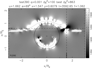
Figure 15: Top panel: OGLE III observations of OGLE-2005-BLG-390. One data point occurs during a planet anomaly. The point-source point-lens (PSPL) model fits 5 parameters, the peak time $t_{0}$, peak magnification $A_{0}$, Einstein radius crossing time $t_{\rm E}$, the source flux $f_{\rm S}$ and blend flux $f_{\rm B}$. Middle panel: Greyscale representation of $\chi^{2}(x,y)$, moving a planet with mass ratio $q=10^{-3}$ on the $(x,y)$ lens plane, holding fixed the 5 PSPL parameters. The $\chi^{2}$ increases by 100 or more in the white areas, where the planet is ruled out, and decreases by 100 or more in the black areas. Bottom panel: The $\chi^{2}(x,y)$ map re-fitting the 5 PSPL parameters for each planet position, showing the smaller size of the resulting planet detection zones.

5.4 Targeting Specific Types of Stars and Planets

As our knowledge of the exo-planet distribution function accumulates, one might contemplate introducing a prior on the parameters $q$, $M_{\star}$, and $a$ in order to target the planet search toward particular types of stars or planets. For example, since $t_{\rm E}\propto M_{\star}^{1/2}$, fast events correspond on average to lower-mass stars. Similarly, since $a\propto t_{\rm E}u_{\pm}$, larger orbits can be targeted by observing slower events and observing longer after the event peak. It is straightforward to tilt the search toward any specific parts of parameter space. However, at this stage our knowledge of the cool planet distribution is so scant that it is probably premature to invest much effort into such fine-tuning.

6 Summary

OGLE III and MOA II are discovering 600-1000 Galactic Bulge microlens events each year. This stretches the resources available for intensive follow-up monitoring of the lightcurves in search of planets near the lens stars. We advocate optimizing microlens planet searches by using an automatic prioritization algorithm based on the planet detection zone area probed by each new data point. We evaluate detection zone areas numerically and validate a plausible scaling law useful for rough but rapid calculations. The proposed optimization scheme takes account of the telescope and detector characteristics, CCD saturation, readout time, and telescope slew time, sky brightness and seeing, past observations of microlensing events underway, and the time available for observing on each night. The current brightness and magnification of each target are estimated by extrapolating fits to previous data points. The optimal observing strategy then provides a recommendation of which targets to observe and which to skip, and a recommended exposure time for each target, designed to maximize the planet detection capability of the observations. This must be coupled with rapid data reduction to trigger continuous follow-up observations whenever an anomaly is detected. It is hoped that the algorithm will provide helpful guidance to follow-up observing teams, and may be a useful starting point for optimising fully-robotic microlens planet searches.

6.1 WEB-PLOP

An implementation of this optimisation scheme, Planet Lens OPtimisation (PLOP or web-PLOP), can be found at http://www.artemis-uk.org/web-PLOP/ [Snodgrass, et al. 2008]. This system was designed with two motivations: to provide an optimal target list for the automated observing of the RoboNet project [Burgdorf, et al. 2007, Tsapras, et al. 2009], and also to provide such lists to human observers at any telescope. It is formed of two parts. First, a user interface web form takes input for the telescope and observing conditions parameters ($A_{\rm eff}$, $t_{\rm slew}$, $t_{\rm read}$, $\mu_{\rm sky}$, $\Delta\theta$ etc.) and the total available observing time, $t$. Secondly, a background code keeps track of the current data on each event (from OGLE, MOA, RoboNet, and all teams that make data available in real time), and produces a new PSPL fit whenever new data arrives. The results from these fits give the event parameters $t_{\rm E}$, $A_{0}$ etc. that are used to predict the magnification at the requested time of observation. These two sets of inputs allow the calculation of $g_{i}$ for each event using Eqn. (69), and therefore an optimal list of targets with suggested exposure times for the requested telescope at the requested time. The list is then put out in either a machine readable or sortable human friendly format. With RoboNet, this output controls the telescope, and new data is fed back into the PSPL model to close the loop and give priorities that are based on data just taken. For human observers at other sites, the output pages are customisable to display any desired parameters along with the priority of each microlensing event, and also show light-curves and detection zone maps along with links to the finding charts and original OGLE and/or MOA pages for each. Although written for RoboNet, this prioritisation tool is freely available and other microlensing observers are encouraged to make use of it.

Acknowledgements

Keith Horne was supported by a PPARC Senior Fellowship during the early stages of this work. We thank Steve Kane, Martin Dominik, Scott Gaudi, and Pascal Fouque for helpful comments on early versions of the manuscript.

References

- [Albrow, et al. 1998] Albrow, M., et al. 1998, ApJ, 509, 687.
- [Beaulieu, et al. 2006] Beaulieu, J.-P., et al. 2006, Nature, 439, 437.
- [Bennett, Andreson, Gaudi 1996] Bennett, D. P., Andrerson, J, Gaudi, B. S., 2007, ApJ 660, 781.
- [Bennett & Rhie 1996] Bennett, D. P., Rhie, S. H. 1996, ApJ, 472, 660.
- [Bennett, et al. 2008] Bennett, D. P., et al. 2008, ApJ, 684, 663.
- [Bond, et al. 2004] Bond, I. A., et al. 2004, ApJ, 606, 155.
- [Burgdorf, et al. 2007] Burgdorf, M.J., et al. 2007, P&SS, 55, 582.
- [Dong, et al. 2009] Dong, S., et al. 2009, ApJ, submitted. (arXiv:0804.1354)
- [Dominik 1998] Dominik, M. 1998, A&A, 333, L79.
- [Dominik, et al. 2007] Dominik, M., et al. 2007, MNRAS, 380, 792.
- [Gaudi, et al. 2002] Gaudi, B. S., et al. 2002, ApJ, 566, 463.
- [Gaudi & Han 2004] Gaudi, B. S., Han, C., 2004, ApJ 611, 528.
- [Gaudi, et al. 2008] Gaudi, B. S., et al. 2008, Science, 319, 927.
- [Gould 2009] Gould, A. 2009, in “The Variable Universe: A Celebration of Bodhan Paczynski”, ed. K.Stanek. ASP Conf. ???, 2009. (arXiv:0803.4324).
- [Gould & Loeb 1992] Gould, A. & Loeb, A. 1992, ApJ, 396, 104.
- [Gould et al. 2006] Gould, A. et al. 2006, ApJ, 644, 37.
- [Griest & Safizadeh 1998] Griest, K. & Safizadeh, N. 1998, ApJ, 500, 37.
- [Jaroszynski & Paczynski 2002] Jaroszynski, M. & Paczynski, B. 2002, Acta. Astron., 52, 361.
- [Krisciunas & Schaefer 1991] Krisciunas, K., Schaefer, B. E., 1991, PASP, 103, 1033.
- [Mao & Paczynski 1991] Mao, S. & Paczynski, B. 1991, ApJ, 304, 1.
- [Patat 2003] Patat, F. 2003, A&A 400, 1183.
- [Rattenbury, et al. 2002] Rattenbury, N. J., Bond, I. A., Skuljan, J., Yock, P. C. M. 2002, MNRAS, 335, 159.
- [Snodgrass, Horne, Tsapras 2004] Snodgrass, C., Horne, K., Tsapras, Y. 2004, MNRAS, 351, 967.
- [Snodgrass, et al. 2008] Snodgrass, C., Tsapras, Y.P., Street, R., Bramich, D., Horne, K., Dominik, M., Allan, A. 2008, in “The Manchester Microlensing Conference: The 12th International Conference and ANGLES Microlensing Workshop”, eds. E. Kerins, S. Mao, N. Rattenbury and L. Wyrzykowski, PoS(GMC8)056. (arXiv:0805.2159).
- [Tsapras, et al. 2003] Tsapras, Y., et al. 2003, MNRAS 343, 1131.
- [Tsapras, et al. 2009] Tsapras, Y., et al. 2009, AN, 330, 4. (arXiv:0808.0813)
- [Udalski, et al. 2003] Udalski, A., 2003, Acta Astron. 53, 291.
- [Udalski, et al. 2005] Udalski, A., et al. 2005, ApJ 628, 109.