Quasiparticles for quantum dot array in graphene and the associated Magnetoplasmons

Abstract

We calculate the low-frequency magnetoplasmon excitation spectrum for a square array of quantum dots on a two-dimensional (2D) graphene layer. The confining potential is linear in the distance from the center of the quantum dot. The electron eigenstates in a magnetic field and confining potential are mapped onto a 2D plane of electron-hole pairs in an effective magnetic field without any confinement. The tight-binding model for the array of quantum dots leads to a wavefunction with inter-dot mixing of the quantum numbers associated with an isolated quantum dot. For chosen confinement, magnetic field, wave vector and frequency, we plot the dispersion equation as a function of the period $d$ of the lattice. We obtain those values of $d$ which yield collective plasma excitations. For the allowed transitions between the valence and conduction bands in our calculations, we obtain plasmons when $d\lesssim 100{\AA}$.

I Introduction

A two-dimensional (2D) honeycomb lattice of carbon atoms that form the basic planar structure in graphite (graphene) has recently been producedNovoselov1 ; Zhang1 . Unusual many-body effects in graphene have been attributed to low-lying excitations in the vicinity of the Fermi levelblinowski ; Shung1 ; Shung2 ; DasSarma . The influence of an external magnetic field on the many-electron properties of graphene results in an unusual quantum Hall effect. The integer quantum Hall effect (IQHE) was discovered in graphene in recent experimentsNovoselov2 ; Zhang2 ; Zhang3 . The quantum Hall ferromagnetism in graphene has been studied theoretically Nomura . In addition, the influence of magnetic field on the Bose-Einstein condensation and superfluidity of indirect magnetoexcitons in graphene bilayer has been studied BLG . The spectrum of plasmon excitations in a single graphene layer immersed in a material with effective dielectric constant $\varepsilon_{b}$ in the absence of magnetic field ($B=0$) was calculated in Refs. Shung1 ; Shung2 ; Hwang . (See also new1 ; new2 ; new3 ; new4 .) The collective plasma excitations in layered graphene structures in high magnetic field were obtained in Ref. berman_gumbs_lozovik where the instability of these modes was investigated. Recently, several works were reported for quantum dots in graphene dots4 ; dots5 ; dots6 . The transport characteristics of quantum dot devices etched entirely in graphene have been studied experimentally Novoselov_dots . According to Ref. Novoselov_dots , these quantum dots at large sizes behave as conventional single-electron transistors. This is just one of the areas of research in the fast-growing field of the electronic transport , thermal and optical properties of graphene which may have important device applications because of its high mobility guinea . The single-particle states and collective modes in semiconductor quantum dots have long been a subject of interest to both theoreticians and experimentalists dots1 ; dots3 ; Maksym . The spectrum of collective plasma modes in a 2D array of quantum dots in semiconductors has been calculated Que .

In this paper, we obtain the dispersion relation for magnetoplasmons in a square array of quantum dots formed by a confining potential which is a linear function of distance from the center of the quantum dot. A perpendicular magnetic field $\mathbf{B}$ is applied. The conditions for the existence of the collective excitations will be investigated.

This paper is organized as follows. In Sec. II, we introduce the quasiparticle electron-hole representation for the eigenvalue problem for an electron in a single graphene quantum dot in magnetic field. In Sec. III we represent the calculations of the magnetoplasmon spectrum in a quantum dot array in graphene. A brief discussion of the results of our calculations plasmon instabilities in graphene is presented in Sec. IV.

II Single-electron States for a graphene quantum dot in magnetic field

We now consider an electron in a graphene layer in the presence of a perpendicular magnetic field $\mathbf{B}$ and a confining potential $U(r^{\prime})=\lambda_{0}|r^{\prime}|$, where $\lambda_{0}>0$ is the slope of the potential. The effective-mass Hamiltonian of an electron in the absence of scatterers in one valley in graphene located in the $xy$-plane is given by a $2\times 2$ matrix Hamiltonian $\hat{H}_{(0)}$ with zero along the diagonal and off-diagonal elements $\hat{\pi}_{x}\mp i\hat{\pi}_{y}$ Ando ; Jain . Here, we neglect the Zeeman splitting and assume energy degeneracy with respect to the two valleys. Also, in our notation, $\hat{\mathbf{\pi}}=-i\hbar\nabla+e\mathbf{A}$, $\mathbf{A}$ is the vector potential of an electron, $v_{F}=\sqrt{3}at/(2\hbar)$ is the Fermi velocity of electrons with $a=2.566\AA$ denoting the lattice constant and $t\approx 2.71eV$ is the overlap integral between nearest-neighbor carbon atoms in graphene Lukose . The eigenvalue problem of an electron in a linear confining potential can be mapped onto one for a noninteracting electron-hole pair in an effective magnetic field $\tilde{B}_{\rm eff}$ under conditions we introduce below.

The eigenfunction $\psi_{\tau}$ for the Hamiltonian $\hat{H}_{(0)}$ for an electron-hole pair in an effective magnetic field $\tilde{B}_{\rm eff}$, is also the eigenfunction of the magnetic momentum $\hat{\mathbf{P}}$ has the form Gorkov ; Lerner ; Kallin and is given by

$$\psi_{\mathbf{P}}(\mathbf{R},\mathbf{r})=\exp\left[\frac{i}{\hbar}\mathbf{R}\cdot\left(\mathbf{P}+e[\tilde{\mathbf{B}}_{\rm eff}\times\mathbf{r}]\right)\right]\tilde{\Phi}(\mathbf{r}-\mathbf{\rho}_{0})\ ,$$ (1)

where $\mathbf{R}=(\mathbf{r}_{e}+\mathbf{r}_{h})/2$, $\mathbf{r}=\mathbf{r}_{e}-\mathbf{r}_{h}$ and $\mathbf{\rho}_{0}=[\tilde{\mathbf{B}}_{\rm eff}\times\mathbf{P}]/(e\tilde{B}_{\rm eff}^{2})$. The cylindrical gauge for vector potential is used with $\mathbf{A}_{e(h)}=1/2[\tilde{\mathbf{B}}_{\rm eff}\times\mathbf{r}_{e(h)}]$. The wavefunction of the relative coordinate $\tilde{\Phi}(\mathbf{r})$ can be expressed in terms of the 2D harmonic oscillator eigenfunctions $\Phi_{n_{1},n_{2}}(\mathbf{r})$. For an electron in Landau level $n_{+}$ and a hole in level $n_{-}$, the four-component wavefunctions for the relative motion in graphene are Fertig

$$\tilde{\Phi}_{n_{+},n_{-}}(\mathbf{r})=\left(\sqrt{2}\right)^{\delta_{n_{+},0}+\delta_{n_{-},0}-2}$$

$$\times\left(\begin{array}[]{c}s_{+}s_{-}\Phi_{|n_{+}|-1,|n_{-}|-1}(\mathbf{r})\\ s_{+}\Phi_{|n_{+}|-1,|n_{-}|}(\mathbf{r})\\ s_{-}\Phi_{|n_{+}|,|n_{-}|-1}(\mathbf{r})\\ \Phi_{|n_{+}|,|n_{-}|}(\mathbf{r})\end{array}\right)\ ,$$ (6)

where $s_{\pm}=\mathrm{sgn}(n_{\pm})$. The corresponding energy of the electron-hole pair $E_{n_{+},n_{-}}$ of the Hamiltonian $\hat{H}_{(0)}$ is given by Fertig

$$E_{n_{+},n_{-}}=\sqrt{2}\ \left((\hbar v_{F}/r_{B}^{\ast})\right)$$

$$\times\left[\mathrm{sgn}(n_{+})\sqrt{|n_{+}|}-\mathrm{sgn}(n_{-})\sqrt{|n_{-}|}\right]\ ,$$ (7)

where $r_{B}^{\ast}=\sqrt{\hbar/(e\tilde{B}_{\rm eff})}$ is an effective magnetic length. The 2D harmonic oscillator wavefunctions $\Phi_{n_{1},n_{2}}(\mathbf{r})$ are given by Fertig

$$\Phi_{n_{1},n_{2}}(\mathbf{r})=(2\pi)^{-1/2}2^{-|m|/2}\frac{\tilde{n}!}{\sqrt{n_{1}!n_{2}!}}\frac{1}{r_{B}^{*}}\mathrm{sgn}(m)^{m}$$

$$\times\frac{r^{|m|}}{r_{B*}^{|m|}}\exp\left[-im\phi-\frac{r^{2}}{4r_{B}^{*2}}\right]L_{\tilde{n}}^{|m|}\left(\frac{r^{2}}{2r_{B}^{*2}}\right)\ ,$$ (8)

where $L_{\tilde{n}}^{|m|}(x)$ is a Laguerre polynomial, $m=n_{1}-n_{2}$, $\tilde{n}=\min(n_{1},n_{2})$ and $\mathrm{sgn}(m)^{m}\to 1$ for $m=0$. The electron-hole eigenfunction given by Eqs. (1), (II), (II) along with the energy eigenvalues are the same as the eigenfunction and the eigenvalue of the Hamiltonian $\hat{H}_{(0)}$ for an electron in a quantum dot in external magnetic field. The magnetic momentum $\mathbf{P}=-e[\tilde{\mathbf{B}}_{\rm eff}\times\mathbf{r}]$ must be the same for the electron and the electron-hole pair at fixed relative coordinate $\mathbf{r}$. The effective magnetic field $\tilde{B}_{\rm eff}$ depends on the slope $\lambda_{0}$ of the confining potential as well as the external magnetic field $B$ and is given by

$$\tilde{B}_{\rm eff}=\left(B^{2}+(4\lambda_{0}^{2}/(e^{2}v_{F}^{2})\right)^{1/2}\ .$$ (9)

In the case when there is no electron confinement, i.e., $\lambda_{0}=0$, the effective magnetic field is the same as the applied magnetic field and $\tilde{B}_{\rm eff}=B$. If there is no external magnetic field, i.e., $B=0$, then there is still an effective magnetic field due to the electron confinement and is given by $\tilde{B}_{\rm eff}=2\lambda_{0}/(ev_{F})$. The coordinate of the electron-hole relative motion $r=|\mathbf{r}_{e}-\mathbf{r}_{h}|$ is related to the distance $r^{\prime}$ of an electron from the center of the confining potential by $r=r^{\prime}/2$.

It should be emphasized that the electrostatic potential for a graphene quantum dot was chosen to have a linear dependence on the coordinate variable $|r^{\prime}|$. This was done because the eigenvalue problem of the Hamiltonian $\hat{H}_{(0)}$ described by the Dirac-like equation with a linear potential can be reduced to the Klein-Gordon-type equation with a parabolic potential $U(r^{\prime})=\lambda_{0}^{2}r^{\prime\ 2}$. This Klein-Gordon-type equation can then be mapped onto the electron-hole problem in an effective magnetic field $\tilde{B}_{\rm eff}$ defined above under the conditions presented.

III Magnetoplasmons for a quantum dot array in graphene

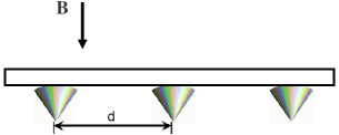
Figure 1: A periodic 2D array of quantum dots in a graphene plane formed by linear confinement with a spacing $d$ in a perpendicular magnetic field $\mathbf{B}$.

We now turn our attention to an infinite periodic 2D array of quantum dots in a graphene plane, shown schematically in Fig. 1. The quantum dots are formed by a periodic linear confining potential defined by $U(r^{\prime})=\sum_{j}\lambda_{0}|\mathbf{r}^{\prime}-\mathbf{r}_{j}|$, where $\mathbf{r}_{j}$ is the position vector of a quantum dot. We consider this array with the period $d$ in a perpendicular magnetic field $\mathbf{B}$ as shown schematically in Fig. 1. For this system, we apply the tight-binding approximation Que ; gumbs ; Bottger (see Eq. (2.1) in Ref. Que )

$$\Psi_{{\bf k}}(x,y)=\left|\mathbf{k},\alpha\right\rangle=\sum_{\mathbf{r}_{j}}e^{i\mathbf{k}\cdot\mathbf{r}_{j}}\psi_{\alpha}(\mathbf{r}-\mathbf{r}_{j})\exp\left(-\frac{ie}{\hbar}\mathbf{A}\cdot\mathbf{r}_{j}\right)\ ,$$ (10)

where $\mathbf{k}$ is an in-plane wave vector, $\psi_{\alpha}$ is the electron eigenfunction in one quantum dot (which can be represented by the wavefunction of an electron-hole pair in an effective magnetic field as $\psi_{\alpha}=\tilde{\Phi}_{n_{+},n_{-}}(\mathbf{r}/2)$, where $\tilde{\Phi}_{n_{+},n_{-}}(\mathbf{r}/2)$ is given by Eq. (II). The index $\alpha=\{n_{+},n_{-}\}$ is a composite quantum number with $n_{+}$ and $n_{-}$ labeling the electron and hole energy levels, respectively. Also, $\mathbf{A}$ is the vector potential for the externally applied magnetic field $\mathbf{B}$.

Note that the electron wave function in periodic systems in a magnetic field is the eigenfunction of both the Hamiltonian and the operator of the magnetic translation. The electronic properties in the presence of magnetic field are determined by the magnetic flux through a unit cell. Thouless If this flux (measured in flux quantum $\phi_{0}=h/e$) is a rational number $\Phi/\phi_{0}=p/q=Ba^{2}e/2\pi\hbar$ where $p$ and $q$ are prime integers, then the electron wave function which is also an eigenfunction of the magnetic translation operator LP obeys the Bloch-Peierls conditions in the Landau gauge which may be expressed asThouless

$$\Psi_{{\bf k}}(x,y)=\Psi_{{\bf k}}(x+qa,y+a)e^{-ik_{x}qa}e^{-ik_{y}a}e^{-2\pi ipy/a}\ .$$ (11)

For integer $m_{1},m_{2}$, the vectors ${\bf a}_{m}(m_{1}qa,n_{2}a)$ define the magnetic lattice of the crystal. The magnetic Brillouin zone is defined by the inequalities $-\pi/qa\leq k_{x}\leq\pi/qa$ and $\pi/a\leq k_{y}\leq k_{y}\leq\pi/a$.

Let us demonstrate that the electron wavefunction given by Eq. (10) obeys the Bloch-Peierls conditions in the Landau gauge. In this gauge, the vector potential may be chosen as ${\bf A}=(0,Bx,0)$. Then, Eq. (10) yields

$$\Psi_{{\bf k}}(x+qa,y+a)=\sum_{\mathbf{r}_{j}}e^{i\mathbf{k}\cdot\mathbf{r}_{j}}\psi_{\alpha}((x+qa)\hat{i}+(y+a)\hat{j}-\mathbf{r}_{j})\exp\left(-\frac{ie}{\hbar}B(x+qa)\hat{j}\cdot\mathbf{r}_{j}\right)\ .$$ (12)

Now, let ${\bf r}_{j}-qa\hat{i}-a\hat{j}={\bf r}_{j}^{\prime}$. Then, Eq. (12) becomes

$$\Psi_{{\bf k}}(x+qa,y+a) = \sum_{\mathbf{r}_{j}^{\prime}}e^{i\mathbf{k}\cdot(\mathbf{r}_{j}^{\prime}+qa\hat{i}+a\hat{j})}\psi_{\alpha}({\bf r}-\mathbf{r}_{j}^{\prime})\exp\left(-\frac{ie}{\hbar}B(x+qa)\hat{j}\cdot(\mathbf{r}_{j}^{\prime}+qa\hat{i}+a\hat{j})\right)$$ (13)

$$= e^{ik_{x}qa}e^{ik_{y}a}\sum_{\mathbf{r}_{j}^{\prime}}e^{i\mathbf{k}\cdot\mathbf{r}_{j}^{\prime}}\psi_{\alpha}(x\hat{i}+y\hat{j}-\mathbf{r}_{j}^{\prime})$$

$$\times \exp\left(\frac{-ie}{\hbar}{\bf A}\cdot{\bf r}_{j}^{\prime}-2\pi ip-2\pi i\frac{p}{q}\frac{x}{a}-2\pi ip\left(\frac{{\bf r}_{j}\cdot\hat{j}}{a}\right)\right)$$

$$= e^{ik_{x}qa}e^{ik_{y}a}\exp\left(-2\pi i\frac{p}{q}\frac{x}{a}\right)\Psi_{{\bf k}}(x,y)\ .$$

But, this result in Eq. (13) is equivalent to Eq. (11). The reason is that they coincide when we rotate axes in the frame before doing the displacement, i.e., $x$-axis $\to-y$-axis or, replacing $x\to-y/q$ on the right-hand-side of Eq. (13). This is now explicitly demonstrated below. Using the gauge ${\bf A}=(-By,0,0)$, we obtain

$$\Psi_{{\bf k}}(x+qa,y+a) = \sum_{\mathbf{r}_{j}^{\prime}}e^{i\mathbf{k}\cdot(\mathbf{r}_{j}^{\prime}+qa\hat{i}+a\hat{j})}\psi_{\alpha}({\bf r}-\mathbf{r}_{j}^{\prime})\exp\left(-\frac{ie}{\hbar}B(-y-a)\hat{i}\cdot(\mathbf{r}_{j}^{\prime}+qa\hat{i}+a\hat{j})\right)$$ (14)

$$= e^{ik_{x}qa}e^{ik_{y}a}\sum_{\mathbf{r}_{j}^{\prime}}e^{i\mathbf{k}\cdot\mathbf{r}_{j}^{\prime}}\psi_{\alpha}(x\hat{i}+y\hat{j}-\mathbf{r}_{j}^{\prime})$$

$$\times \exp\left(\frac{-ie}{\hbar}{\bf A}\cdot{\bf r}_{j}^{\prime}+2\pi ip+2\pi ip\frac{y}{a}+2\pi i\frac{p}{q}\left(\frac{{\bf r}_{j}\cdot\hat{i}}{a}\right)\right)$$

$$= e^{ik_{x}qa}e^{ik_{y}a}\exp\left(2\pi ip\frac{y}{a}\right)$$

$$\times \sum_{\mathbf{r}_{j}^{\prime}}e^{i\mathbf{k}\cdot\mathbf{r}_{j}^{\prime}}\psi_{\alpha}(x\hat{i}+y\hat{j}-\mathbf{r}_{j}^{\prime})\exp\left\{2\pi i\frac{p}{q}\left(\frac{{\bf r}_{j}^{\prime}\cdot\hat{i}}{a}\right)\right\}\ .$$

The last line in Eq. (14) satisfies the Eq. (11) perfectly if we take ${\bf k}$ to be ${\bf k}$ modulo $2\pi/aq$. Therefore, we conclude that the electron wavefunction given by Eq. 10 obeys the Bloch-Peierls conditions in the Landau gauge. In Ref. [Perov, ] quantum states of a similar system were considered. The energy spectrum in this case consists of magnetic subbands defined in a magnetic Brillouin zone. The structure of magnetic subband depends on the number of magnetic flux penetrating the unit cell. The wave function given by Eq. (10) corresponds to one in Ref. [Perov, ] if we do not include spin-orbit coupling in our model.

We do not consider magnetic fields where the flux is $p/q$ in our numerical calculation, since this would involve a formalism like the one presented in Refs. [gumbs2, ; gumbs3, ]. Furthermore, the resulting fractal nature of the energy spectrum under these conditions can only be realized numerically for magnetic fields which are several tens of Tesla. This is beyond the interest and scope of the present paper.

Following the procedure adopted in Ref. Que , we introduce the quantity

$$\Pi_{\alpha\beta}(\omega) = \left(\frac{g_{s}g_{v}}{2\pi r_{B}^{\ast\ 2}}\right)\frac{f_{0}(E_{\alpha})-f_{0}(E_{\beta})}{\hbar\omega+E_{\alpha}-E_{\beta}+i0^{+}}\ ,$$ (15)

where $g_{s}=2$ and $g_{v}=2$ are the spin and valley degeneracies in graphene, $\omega$ denotes frequency, $\alpha=(n_{+},n_{-})$, $\beta=(n_{+}^{\prime},n_{-}^{\prime})$, $E_{\alpha(\beta)}$ are the electron-hole pair eigenenergies for the Landau levels in an effective magnetic field. Also, $f_{0}(E)$ is the occupation function of the two-particle state. At high temperatures or weak magnetic field, when the separation between Landau levels is small so that $k_{B}T\gg\hbar v_{F}/r_{B}^{\ast}$, the occupation of the Landau levels is given by the Fermi-Dirac distribution function $f_{0}(E_{\alpha})=\left(\exp\left[E_{\alpha}/(k_{B}T)\right]+1\right)^{-1}$.

We now introduce the overlap integral $F_{\alpha\beta}(\mathbf{q})$ involving the eigenstates with labels $\alpha=\{n_{+},n_{-}\}$ and $\beta=\{n_{+}^{\prime},n_{-}^{\prime}\}$ through the equation Que

$$F_{\alpha\beta}(\mathbf{q})=\int d^{2}\mathbf{r}\ e^{i\mathbf{q}\cdot\mathbf{r}}\psi_{\alpha}^{\ast}(\mathbf{r})\psi_{\beta}(\mathbf{r})=s_{+}s_{+}^{\prime}s_{-}s_{-}^{\prime}\$$

$$\times F_{|n_{+}|-1,|n_{-}|-1,|n_{+}^{\prime}|-1,|n_{-}^{\prime}|-1}^{(0)}(\mathbf{q})$$

$$+s_{+}s_{+}^{\prime}\ F_{|n_{+}|-1,|n_{-}|,|n_{+}^{\prime}|-1,|n_{-}^{\prime}|}^{(0)}(\mathbf{q})$$

$$+s_{-}s_{-}^{\prime}\ F_{|n_{+}|,|n_{-}|-1,|n_{+}^{\prime}|,|n_{-}^{\prime}|-1}^{(0)}(\mathbf{q})$$

$$+F_{|n_{+}|,|n_{-}|,|n_{+}^{\prime}|,|n_{-}^{\prime}|}^{(0)}(\mathbf{q})\ ,$$ (16)

where

$$F_{n_{1},n_{2},n_{1}^{\prime},n_{2}^{\prime}}^{(0)}(\mathbf{q})=\int d^{2}\mathbf{r}\ e^{i\mathbf{q}\cdot\mathbf{r}}\Phi_{n_{1}^{\prime},n_{2}^{\prime}}^{\ast}(\mathbf{r})\Phi_{n_{1},n_{2}}(\mathbf{r})$$ (17)

and $\Phi_{n_{1},n_{2}}(\mathbf{r})$ is given by Eq. (II). The angular integral in Eq. (17) can be carried out using the result

$$\int_{0}^{2\pi}d\theta\ e^{i\beta\cos(\theta)-im\theta}=2\pi(-i)^{m}J_{m}(-\beta)$$ (18)

with $m$ an integer. If $m$ is even, $J_{m}(-\beta)=J_{m}(\beta)$.

We employ the procedure introduced in Ref. Que for determining the dispersion relation $\omega=\omega(\mathbf{q})$ for the magnetoplasmon excitation frequencies. This can be calculated from the condition of the vanishing of the determinant of the matrix with elements $C_{ij}(\mathbf{q},\omega)$. In this notation, the subscript $i$ denotes the pair of quantum numbers $\alpha$ and $\beta$ for two different composite electron-hole pairs. Also, $j$ denotes the quantum numbers $\alpha^{\prime}$ and $\beta^{\prime}$ for two other composite electron-hole pairs. The matrix elements $C_{ij}$ are defined as

$$C_{ij}(\mathbf{q},\omega)=\delta_{ij}$$

$$-\Pi_{i}(\omega)\sum_{\mathbf{G}}\frac{2\pi e^{2}}{\varepsilon_{s}|\mathbf{q}+\mathbf{G}|}F_{i}(\mathbf{q}+\mathbf{G})F_{j}^{\ast}(\mathbf{q}+\mathbf{G})\ .$$ (19)

In this notation, $\varepsilon_{s}=4\pi\epsilon_{0}\epsilon_{b}$, where $\epsilon_{b}$ is the average dielectric constant of the medium where the layer of graphene is embedded. We also introduced $\mathbf{G}=2\pi/d\left(n_{x},n_{y}\right)$ which is a reciprocal lattice vector of the square array of quantum dots with period $d$ and $n_{x},\ n_{y}=0,\pm 1,\pm 2,\cdots$.

In solving the dispersion equation for plasmon excitations, we chose the slope of the confining potential, magnetic field, wave vector, frequency, temperature and background dielectric constant. We then varied the period $d$ and calculated the determinant $\det[C_{ij}(\mathbf{q},\omega)]$ obtained from Eq. (III). The zeros of the determinant correspond to the collective magnetoplasmon excitations. As is shown in Fig. 2, allowed plasmon resonances appear in the system at specific values of the dot spacing $d$ corresponding to the condition $\det[C_{ij}(\mathbf{q},\omega)]=0$. The results of these calculations were obtained by taking into account only transitions between the Landau levels $n=-1,0,1$ . The interdot separations where the plasmons can be excited are given by $d\lesssim 100{\AA}$. The excitation spectrum of the collective modes preserves the periodicity of the lattice, even with the mixing of the quantum numbers.

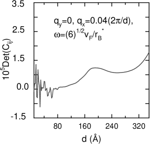
Figure 2: $\det[C_{ij}(\mathbf{q},\omega)]$ as a function of an array spacing $d$ calculated using Eq. (III). We chose the slope of the confinement $\lambda_{0}=10^{-2}eV/{\AA}$, magnetic field $B=1T$, $\epsilon_{b}=2.5$ and the temperature T=0 K. The values of spacing $d$ resulting in $\det[C_{ij}(\mathbf{q},\omega)]=0$ correspond to the existence of magnetoplasmon excitations at chosen frequency and wave vector.

IV Discussion

In Fig. 3, we present the dispersion relation for plasmons in a 2D array of quantum dots in a perpendicular magnetic field at zero temperature. The parameters used in the calculation are given in the figure. The frequency is plotted as a function of $q_{x}$ with $q_{y}=0$. As $q_{x}$ increases in the long wavelength limit, the group velocity is initially small but then rapidly becomes negative for a range of wave vector. Then, over a narrow range of wave vector, the frequency increases before it again decreases as it approaches the Brillouin zone boundary. The finite frequency of excitation in the long wavelength limit is due to the allowed transition between the valence and conduction band. In calculating the dispersion, we must solve for the zeros of the $(2N+1)^{4}\times(2N+1)^{4}$-dimensional $\det[C_{ij}(\mathbf{q},\omega)]$ as a function of frequency, where $i,j=0,\pm 1,\pm 2,\cdots,\pm N$ are the energy level labels in the valence and conduction bands. Thus, when we include the $0,\pm 1$ levels only, the determinant has dimension eighty-one. We note that the negative dispersion must be due to the effective magnetic field since the group velocity is always positive for a graphene sheet in the absence of magnetic field Shung1 ; DasSarma ; new4 . The commensurability effect between the electron cyclotron orbits and the period of the quantum dot array can be explained by the oscillations in the plasma dispersion shown in Fig. 3. The interaction term decreases as the wave vector increases, thereby resulting in the decrease in plasmon excitation energy as $q_{x}$ approaches the Brillouin zone boundary. Since each value of inter-dot separation has its own set of eigenstates, the dispersion relation could be drastically changed by choosing a different value of $d$. We note that a zero-gap graphite sheet only excites the inter-band electron-hole excitations at zero temperature. At finite temperature, there will be intra-band excitations which induce intra-band plasmon modes.

In summary, the methodological achievement of the approach presented in this paper is the mapping of the single-electron eigenfunctions (Eq. (II)) and eigenenergies in magnetic field in linear confinement in graphene onto the eigenfunctions and eigenenergies of a new set of quasiparticles of quasielectrons and quasiholes, without confinement in an effective magnetic field depending on the slope of the confinement. The quasiparticle technique is also well suited for calculating the different linear responses (e.g., conductivity, linear paramagnetic susceptibility, optical response, etc.) which can be found by computing the average $\langle G^{R}(\omega,{\bf r})G^{A}(\omega,-{\bf r},)\rangle$ involving the retarded and advanced Green’s functions. Also, the calculation of the electronic heat capacity, which, as usual, is found from the the temperature derivative of the mean energy, utilizes the quasiparticle energies. Thus. the scope of application of the quasiparticle concept is wide and can be employed in both transport, thermodynamic and optical studies. We showed that the dispersion equation yields allowed plasmon excitations for specific inter-dot separation at chosen wave vector and frequency. Our dispersion curve shows negative group velocity which is generated by the effective magnetic field arising from the external magnetic field and confining potential.

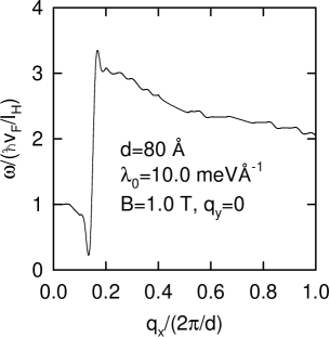
Figure 3: We show in this figure the plasmon excitation frequency as a function of $q_{x}$ for $q_{y}=0$. The slope of the confinement $\lambda_{0}=10^{-2}eV/{\AA}$, magnetic field $B=1T$, $\epsilon_{b}=2.5$ and the temperature T=0 K.

References

- (1) K. S. Novoselov et al., Science 306, 666 (2004).
- (2) Y. Zhang, J. P. Small, M. E. S. Amori, and P. Kim, Phys. Rev. Lett. 94, 176803 (2005).
- (3) J. Blinowski, N. H. Hau, C. Rigaux, J. P. Vieren, R. L. Toullee, G. Furdin, A. Herold and J. Melin, J. Phys. (Paris) 41, 47 (1980).
- (4) Kenneth W. -K. Shung, Phys. Rev. B34, 979 (1986).
- (5) Kenneth W. -K. Shung, Phys. Rev. B34, 1264 (1986).
- (6) S. Das Sarma, E. H. Hwang, and W.- K. Tse, Phys. Rev. B75, 121406(R) (2007).
- (7) K. S. Novoselov et al., Nature (London) 438, 197 (2005).
- (8) Y. B. Zhang et al., Nature (London) 438, 201 (2005).
- (9) Y. Zhang et al., Phys. Rev. Lett. 96, 136806 (2006).
- (10) K. Nomura and A. H. MacDonald, Phys. Rev. Lett. 96, 256602 (2006).
- (11) O. L. Berman, Yu. E. Lozovik and G. Gumbs, Phys. Rev. B77, 155433 (2008).
- (12) S. Das Sarma and E. H. Hwang, Phys. Rev. Lett. 81, 4216 (1998).
- (13) S. Gangadharaiah, A. M. Farid, and E. G. Mishchenko, Phys. Rev. Lett. 100, 166802 (2008).
- (14) B. Wunsch, T. Stauber, F. Sols, F. Guinea, New Journal of Physics 8, 318 (2006).
- (15) M. F. Lin, C. S. Huang, and D. S. Chuu, Phys. Rev. B55, 13961 (1997).
- (16) Ming-Fa Lin and Feng-Lin Shyu, Jour. Phys. Soc. Japan 69, 607 (2000).
- (17) O. L. Berman, G. Gumbs and Yu. E. Lozovik, Phys. Rev. B78, 085401 (2008).
- (18) Milton Pereira, P. Vasilopoulos, and F. M. Peeters, Nano Lett. 7, 946 (2007).
- (19) N. M. R. Peres, A. H. Castro Neto, F. Guinea, Phys. Rev. B73, 241403(R) (2006).
- (20) P. G. Silvestrov and K. B. Efetov, Phys. Rev. Lett. 98, 016802 (2007).
- (21) L. A. Ponomarenko, F. Schedin, M. I. Katsnelson, R. Yang, E. H. Hill, K. S. Novoselov, and A. K. Geim, Science 320, 356 (2008).
- (22) A. H. Castro Neto, F. Guinea, N. M. R. Peres, K. S. Novoselov, and A. K. Geim, Arxiv; 0709.1163v1 (2007).
- (23) L. Brey, N. F. Johnson, and B. I. Halperin, Phys. Rev. B40, 10647 (1989).
- (24) F. M. Peeters, Phys. Rev. B42, 1486 (1990).
- (25) P. A. Maksym and T. Chakraborty, Phys. Rev. Lett. 65, 108 (1990).
- (26) W. Que, G. Kirczenow, and E. Castano, Phys. Rev. B43, 14079 (1991).
- (27) Y. Zheng and T. Ando, Phys. Rev. B65, 245420 (2002).
- (28) C. Tőke, P. E. Lammert, V. H. Crespi, and J. K. Jain, Phys. Rev. B74, 235417 (2006).
- (29) V. Lukose, R. Shankar, and G. Baskaran, Phys. Rev. Lett. 98, 116802 (2007).
- (30) L. P. Gorkov and I. E. Dzyaloshinskii, JETP 26, 449 (1967).
- (31) I. V. Lerner and Yu. E. Lozovik, JETP 51, 588 (1980).
- (32) C. Kallin and B. I. Halperin, Phys. Rev. B30, 5655 (1984); Phys. Rev. B31, 3635 (1985).
- (33) A. Iyengar, J. Wang, H. A. Fertig, and L. Brey, Phys. Rev. B75, 125430 (2007).
- (34) D. Huang and G. Gumbs, Phys. Rev. Lett. B 46, 4147 (1992).
- (35) H. Böttger and V. V. Bryksin, Hopping Conduction in Solids (Akademie-Verlag, Berlin, 1985).
- (36) D. J. Thouless, M. Kohmoto, M. P. Nightingale, and M. den Nijs, Phys. Rev. Lett. 49, 405 (1982).
- (37) E. M. Lifshitz and L. P. Pitaevskii, Course of Theoretical Physics, Vol. 9: Statistical Physics, Part II, (Moscow, Nauka, 1978; Pergamon, New York, 1980).
- (38) V. Ya. Demikhovskii and A. A. Perov, Phys. Rev. B75, 205307 (2007).
- (39) G. Gumbs, D. Miessein, and D. Huang, Phys. Rev. B52, 14755 (1995).
- (40) G. Gumbs and P. Fekete, Phys. Rev. B56, 3787 (1997).