Re-evaluation of the T2KK physics potential
with simulations including backgrounds

Abstract

The Tokai-to-Kamioka-and-Korea (T2KK) neutrino oscillation experiment under examination can have a high sensitivity to determine the neutrino mass hierarchy for a combination of relatively large ($\sim 3.0^{\circ}$) off-axis angle beam at Super-Kamiokande (SK) and small ($\sim 0.5^{\circ}$) off-axis angle at $L\sim 1,000$ km in Korea. We elaborate previous studies by taking into account smearing of reconstructed neutrino energy due to finite resolution of electron or muon energies, nuclear Fermi motion and resonance production, as well as the neutral current $\pi^{0}$ production background to the $\nu_{\mu}\to\nu_{e}$ oscillation signal. It is found that the mass hierarchy pattern can still be determined at $3\sigma$ level if $\sin^{2}2\theta_{\scriptscriptstyle{\rm RCT}}\equiv 4|U_{e3}|^{2}(1-|U_{e3}|^{2})~{}{\hbox to0.0pt{\lower 3.5pt\hbox{$\mathchar 0\relax\sim$}\hss}\raise 1.0pt\hbox{$>$}}\,0.08~{}(0.09)$ when the hierarchy is normal (inverted) with $5\times 10^{21}$ POT exposure, or 5 years of the T2K experiment, if a 100 kton water $\check{\rm C}$erenkov detector is placed in Korea. The $\pi^{0}$ backgrounds deteriorate the capability of the mass hierarchy determination, whereas the events from nuclear resonance productions contribute positively to the hierarchy discrimination power. We also find that the $\pi^{0}$ backgrounds seriously affect the CP phase measurement. Although $\delta_{\scriptscriptstyle{\rm MNS}}$ can still be constrained with an accuracy of $\sim\pm 45^{\circ}$ ($\pm 60^{\circ}$) at $1\sigma$ level for the normal (inverted) hierarchy with the above exposure if $\sin^{2}2\theta_{\scriptscriptstyle{\rm RCT}}~{}{\hbox to0.0pt{\lower 3.5pt\hbox{$\mathchar 0\relax\sim$}\hss}\raise 1.0pt\hbox{$>$}}\,0.04$, CP violation can no longer be established at $3\sigma$ level even for $\delta_{\scriptscriptstyle{\rm MNS}}=\pm 90^{\circ}$ and $\sin^{2}2\theta_{\scriptscriptstyle{\rm RCT}}=0.1$. About four times higher exposure will be needed to measure $\delta_{\scriptscriptstyle{\rm MNS}}$ with $\pm 30^{\circ}$ accuracy.

KEK-TH-1268

1 Introduction

The SNO experiment found that the $\nu_{e}$ from the sun changes into the other active neutrinos [1]. The atmospheric neutrino observation at SK reported that $\nu_{\mu}$ and $\bar{\nu}_{\mu}$ oscillate into the other active neutrinos [2]. Recently, the MiniBooNE experiment [3] reported that the LSND [4] observation of rapid $\bar{\nu}_{\mu}\to\bar{\nu}_{e}$ oscillation has not been confirmed. Consequently, the three active neutrinos are sufficient to describe all the observed neutrino oscillation phenomena.

Under the three generation framework, neutrino flavor oscillation [5, 6] is governed by 2 mass-squared differences and 4 independent parameters in the MNS (Maki-Nakagawa-Sakata) matrix [5], that is 3 mixing angles and 1 CP phase ($\delta_{\scriptscriptstyle{\rm MNS}}{}$). The absolute value of the larger mass-squared difference, $|\delta m^{2}_{13}|$ and one combination of the MNS matrix elements $\sin^{2}2\theta_{\scriptscriptstyle{\rm ATM}}\equiv 4|U_{\mu 3}|^{2}(1-|U_{\mu 3}|^{2})$, are determined by the atmospheric neutrino observation [7, 8, 2, 9], which have been confirmed by the accelerator based long baseline neutrino oscillation experiments K2K [10] and MINOS [11]. However, the sign of $\delta m^{2}_{13}\equiv m^{2}_{3}-m^{2}_{1}$ has not been determined. Both the magnitude and the sign of the smaller mass-squared difference $\delta m^{2}_{12}=m^{2}_{2}-m^{2}_{1}$, another combination of the MNS matrix elements $\sin^{2}2\theta_{\scriptscriptstyle{\rm SOL}}\equiv 4|U_{e1}U_{e2}|^{2}$ are determined by the solar neutrino observations [12, 1] and the KamLAND experiment [13]. The last independent mixing angle ($\theta_{\scriptscriptstyle{\rm RCT}}$) has not been measured yet, and the reactor experiments [14] give upper bound on the combination $\sin^{2}2\theta_{\scriptscriptstyle{\rm RCT}}\equiv 4|U_{e3}|^{2}(1-|U_{e3}|^{2})$. The leptonic CP phase, $\delta_{\scriptscriptstyle{\rm MNS}}{}=-\mbox{arg}U_{e3}$ [15], is unknown.

There are many experiments which plan to measure the unknown parameters of the three neutrino model. In the coming reactor experiments, Double CHOOZ [16], Daya Bay [17], and RENO [18] plan to measure the unknown element $|U_{e3}|$ from the $\bar{\nu}_{e}$ survival probability. The Tokai-to-Kamioka (T2K) neutrino oscillation experiment [19], which is one of the next generation accelerator based long baseline experiments, also plans to measure $|U_{e3}|$ by observing the $\nu_{\mu}\to\nu_{e}$ transition event, whose rate is proportional to $|U_{e3}U_{\mu 3}|^{2}$.

However, the sign of $\delta m^{2}_{13}$, or the mass hierarchy pattern, will remain undetermined even after these experiments. It is not only one of the most important parameters in particle physics but also has serious implications in astronomy and cosmology. For instance, if $\delta m^{2}_{13}$ is negative (inverted hierarchy), the prospects of observing the neutrino-less double beta decay are good, while the matrix element $|U_{e2}|$ is affected by quantum corrections such that its high energy scale value depends on the Majorana phases [20] in the large $\tan\beta$ supersymmetric See-Saw scenario [21]. In astronomy, the mass hierarchy pattern affects the light elements synthesis in the supernova through neutrino-nucleon interactions; the yields of ⁷Li and ¹¹Be increase for the normal hierarchy ($\delta m^{2}_{13}>0$) if $\sin^{2}2\theta_{\scriptscriptstyle{\rm RCT}}~{}{\hbox to0.0pt{\lower 3.5pt\hbox{$\mathchar 0\relax\sim$}\hss}\raise 1.0pt\hbox{$>$}}\,10^{-3}$ [22]. In cosmology, the dark matter content of the universe depends on the mass hierarchy.

In the previous studies [23, 24, 25], we explored the physics impacts of the idea [26] of placing an additional far detector in Korea along the T2K neutrino beam line, which is now called as the T2KK (Tokai-to-Kamioka-and-Korea) experiment. In particular, we studied semi-quantitatively the physics impacts of placing a 100 kton water $\check{\rm C}$erenkov detector in Korea, about $1000$ km away from J-PARC (Japan Proton Accelerator Research Complex) [27], during the T2K experiment period [19], which plans to accumulate $5\times 10^{21}$ POT (protons on target) in 5 years. We find that the neutrino-mass hierarchy pattern can be determined by comparing the $\nu_{\mu}\to\nu_{e}$ transition probability measured at SK ($L=295$ km) and that at a far detector in Korea [23], if $\sin^{2}2\theta_{\scriptscriptstyle{\rm RCT}}~{}{\hbox to0.0pt{\lower 3.5pt\hbox{$\mathchar 0\relax\sim$}\hss}\raise 1.0pt\hbox{$>$}}\,0.05$ for $3\sigma$. The CP phase can also be measured if $\sin^{2}2\theta_{\scriptscriptstyle{\rm RCT}}~{}{\hbox to0.0pt{\lower 3.5pt\hbox{$\mathchar 0\relax\sim$}\hss}\raise 1.0pt\hbox{$>$}}\,0.02$ with $\pm 30^{\circ}$ accuracy, since the amplitude and the oscillation phase of the $\nu_{\mu}\to\nu_{e}$ transition probability are sensitive to $\sin\delta_{\scriptscriptstyle{\rm MNS}}$ and $\cos\delta_{\scriptscriptstyle{\rm MNS}}$, respectively [23, 24]. We also find that the octant degeneracy between $\sin^{2}\theta_{\scriptscriptstyle{\rm ATM}}=0.4$ and $0.6$ for $\sin^{2}2\theta_{\scriptscriptstyle{\rm ATM}}=0.96$ can be resolved if $\sin^{2}2\theta_{\scriptscriptstyle{\rm RCT}}~{}{\hbox to0.0pt{\lower 3.5pt\hbox{$\mathchar 0\relax\sim$}\hss}\raise 1.0pt\hbox{$>$}}\,0.12$ [25]. In the above studies [23, 24, 25], a combination of $3.0^{\circ}$ OAB (off-axis beam) at SK and $0.5^{\circ}$ OAB at $L=1000$ km in Korea is found to be most efficient, mainly because of the hard neutrino spectrum of the $0.5^{\circ}$ OAB. In alternative studies [28] of the T2KK setup, an idea of placing two identical detectors at the same off-axis angle in Kamioka and Korea has been examined. The idea of placing far and very far detectors along one neutrino baseline has also been studied for the Fermi Lab. neutrino beam [29].

The T2KK experiment has a potential of becoming the most economical experiment to determine the mass hierarchy and the CP phase, if $\sin^{2}2\theta_{\scriptscriptstyle{\rm RCT}}$ is not too small. In this paper, we re-evaluate the T2KK physics potential by taking into account smearing of the reconstructed neutrino energy due to finite resolution of electron or muon energies and the Fermi motion of the target nucleon, as well as those events from the nuclear resonance production which cannot be distinguished from the quasi-elastic events by water $\check{\rm C}$erenkov detectors. We also study contribution from the neutral current $\pi^{0}$ production processes which can mimic the $\nu_{e}$ appearance signal.

This article is organized as follows. In section 2, we fix our notation and give approximate analytic expressions for the neutrino oscillation probabilities including the matter effect. The relations between the experimental observables and the three neutrino model parameters are then explained by using the analytic formulas. In section 3, we show how we estimate the event numbers from the charged current (CC) and neutral current (NC) interactions by using the event generator nuance [30]. In section 4, we present the $\chi^{2}$ function which we adopt in estimating the statistical sensitivity of the T2KK experiment on the neutrino oscillation parameters. In section 5, we show our results on the mass hierarchy determination. In section 6, we show our results on the CP phase measurement. In section 7, we give the summary and conclusion. In Appendix Appendix A, we present a parameterization of the reconstructed neutrino energy distribution as a function of the initial neutrino energy for CCQE and resonance events.

2 Notation and approximate formulas

In this section, we fix our notation and present an analytic approximation for the neutrino oscillation probabilities that is useful for understanding the physics potential of the T2KK experiment qualitatively.

2.1 Notation

The neutrino flavor eigenstate $\left|\nu_{\alpha}\right\rangle$ ($\alpha=e,\mu,\tau$) is a mixture of the mass eigenstates $\left|\nu_{i}\right\rangle$ ($i=1,2,3$) with the mass $m_{i}$ as

$$\left|\nu_{\alpha}\right\rangle=\sum^{3}_{i=1}U_{\alpha i}\left|\nu_{i}\right\rangle\,,$$ (1)

where $U$ is the unitary MNS (Maki-Nakagawa-Sakata) [5] matrix. We adopt a convention where $U_{e1}$, $U_{e2}$, $U_{\mu 3}$, $U_{\tau 3}\geq 0$ and $\delta_{\scriptscriptstyle{\rm MNS}}\equiv-\arg U_{e3}$ [15, 31]. The 4 parameters, $U_{e2}$, $U_{\mu 3}$, $\left|U_{e3}\right|$, and $\delta_{\scriptscriptstyle{\rm MNS}}$, can then be chosen as the independent parameters of the $3\times 3$ MNS matrix. All the other elements are determined uniquely by the unitarity conditions [31].

The atmospheric neutrino observation [7, 8, 2, 9] and the accelerator based long baseline experiments [10, 11], which measure the $\nu_{\mu}$ survival probability, are sensitive to the magnitude of the larger mass-squared difference and $\sin^{2}2\theta_{\scriptscriptstyle{\rm ATM}}$ [11]:

$$\sin^{2}2\theta_{\scriptscriptstyle{\rm ATM}} > 0.90~{}~{}~{}{{\mbox{{($90\%$ C.L.)}}}}\,,$$ (2a)

$$|\delta m^{2}_{13}| = (2.43\pm 0.13)\times 10^{-3}{\mbox{{eV}}}^{2}\,.$$ (2b)

The reactor experiments, which observe the survival probability of $\bar{\nu}_{e}$ at $L\sim O(1)$ km, are sensitive to $|\delta m^{2}_{13}|$ and $\sin^{2}2\theta_{\scriptscriptstyle{\rm RCT}}$. The CHOOZ experiment [14] finds

$$\sin^{2}2\theta_{\scriptscriptstyle{\rm RCT}} < (0.20,~{}0.16,~{}0.14)$$ (3a)

$$\mbox{{for~{}~{}~{}}}\left|\delta m^{2}_{13}\right| = (2.0,~{}2.5,~{}3.0)\times 10^{-3}\mbox{{eV}}^{2}\,,$$ (3b)

at the 90% confidence level.

The solar neutrino observations [12], and the KamLAND experiment [13], which measure the survival probability of $\nu_{e}$ and $\bar{\nu}_{e}$, respectively, at much longer distances are sensitive to the smaller mass-squared difference, $\delta m^{2}_{12}$, and $U_{e2}$. The combined results [13] find

$$\sin^{2}2\theta_{\scriptscriptstyle{\rm SOL}} = 0.87\pm 0.04\,,$$ (4a)

$$\delta m^{2}_{12} = (7.59\pm 0.21)\times 10^{-5}{\mbox{{eV}}}^{2}\,.$$ (4b)

The sign of $\delta m^{2}_{12}$ has been determined by the matter effect inside the sun [32].

With a good approximation [33], we can relate the above three mixing factors, eqs. (2a), (3a), (4a) with the elements of the $3\times 3$ MNS matrix;

$$\sin\theta_{\scriptscriptstyle{\rm ATM}} = U_{\mu 3}=\sin\theta_{23}\cos\theta_{13}\,,$$ (5a)

$$\sin\theta_{\scriptscriptstyle{\rm RCT}} = |U_{e3}|=\sin\theta_{13}\,,$$ (5b)

$$\sin 2\theta_{\scriptscriptstyle{\rm SOL}} = 2U_{e1}U_{e2}=\sin 2\theta_{12}\cos^{2}\theta_{13}\,,$$ (5c)

​​​where the three mixing angles $\theta_{ij}=\theta_{ji}$ are defined in the region $0\leq\theta_{12},\theta_{13},\theta_{23}\leq\pi/2$ [15]. In the following, we adopt $\sin\theta_{\scriptscriptstyle{\rm ATM}}$, $\sin\theta_{\scriptscriptstyle{\rm RCT}}$, and $\sin\theta_{\scriptscriptstyle{\rm SOL}}$ as defined above as the independent real mixing parameters of the $3\times 3$ MNS matrix.

2.2 Approximate formulas

The probability that an initial flavor eigenstate $\left|\nu_{\alpha}\right\rangle$ with energy $E_{\nu}$ is observed as a flavor eigenstate $\left|\nu_{\beta}\right\rangle$ after traveling a distance $L$ in the matter of density $\rho(x)$ $(0<x<L)$ along the baseline is

$$P_{\nu_{\alpha}\to\nu_{\beta}} = \left|\left\langle\nu_{\beta}\right|\exp\left({-i\int_{0}^{L}H(x)dx}\right)\left|\nu_{\alpha}\right\rangle\right|^{2}\,,$$ (6)

where the Hamiltonian inside the matter is

$$H(x) = \displaystyle\frac{1}{2E_{\nu}}U\left(\begin{array}[]{ccc}0&0&0\\ 0&\delta m^{2}_{12}&0\\ 0&0&\delta m^{2}_{13}\end{array}\right)U^{\dagger}+\displaystyle\frac{a(x)}{2E_{\nu}}\left(\begin{array}[]{ccc}1&0&0\\ 0&0&0\\ 0&0&0\end{array}\right)\,,$$ (13)

$$= \displaystyle\frac{1}{2E_{\nu}}{\tilde{U}(x)}\left(\begin{array}[]{ccc}\lambda_{1}(x)&0&0\\ 0&\lambda_{2}(x)&0\\ 0&0&\lambda_{3}(x)\end{array}\right){\tilde{U}}^{\dagger}(x)\,,$$ (17)

with

$$a(x)\equiv 2\sqrt{2}G_{F}E_{\nu}n_{e}(x)\simeq 7.56\times 10^{-5}\mbox{{[eV${}^{2}$]}}\left(\displaystyle\frac{\rho(x)}{\mbox{{g/cm${}^{3}$}}}\right)\left(\displaystyle\frac{E_{\nu}}{\mbox{{GeV}}}\right)\,.$$ (18)

Here $G_{F}$ is the Fermi constant, $E_{\nu}$ is the neutrino energy, $n_{e}(x)$ is the electron number density, and $\rho(x)$ is the matter density along the baseline. In the translation from $n_{e}(x)$ to $\rho(x)$, we assume that the number of the neutron is same as that of proton. To a good approximation [19, 34], the matter profile along the T2K and T2KK baselines can be replaced by a constant, $\rho(x)=\rho_{0}$, and the probability eq. (6) can be expressed compactly by using the eigenvalues $(\lambda_{i})$ and the unitary matrix $\tilde{U}$ of eq. (17);

$$P_{\nu_{\alpha}\to\nu_{\beta}} = {\delta}_{\alpha\beta}-4\sum_{i>j}{\rm Re}({\tilde{U}}^{\ast}_{\alpha i}{\tilde{U}}_{\beta i}{\tilde{U}}_{\alpha j}{\tilde{U}}^{\ast}_{\beta j})\sin^{2}\displaystyle\frac{{\tilde{\Delta}}_{ij}}{2}+2\sum_{i>j}{\rm Im}({\tilde{U}}^{\ast}_{\alpha i}{\tilde{U}}_{\beta i}{\tilde{U}}_{\alpha j}{\tilde{U}}^{\ast}_{\beta j})\sin{\tilde{\Delta}}_{ij}\,,~{}~{}~{}~{}~{}~{}$$ (19a)

$$\tilde{\Delta}_{ij} \equiv \displaystyle\frac{\lambda_{j}-\lambda_{i}}{2E}L\,.$$ (19b)

All our numerical results are based on the above solution eq. (19a), leaving discussions of the matter density profile along the baselines to a separate report [34]. Our main results are not affected significantly by the matter density profile [34] as long as the mean matter density along the baseline $(\rho_{0})$ is chosen appropriately.

Although the expression eq. (19a) is not particularly illuminating, we find the following approximations [23, 24] useful for the T2KK experiment. Since the matter effect is small at sub GeV to a few GeV region for $\rho\sim 3$ g/cm³, and the phase factor $\Delta_{12}$ in the vacuum, where

$${\Delta}_{ij}\equiv\displaystyle\frac{m^{2}_{j}-m^{2}_{i}}{2E}L\,,$$ (20)

is also small near the first oscillation maximum, $|\Delta_{13}|\sim\pi$, the approximation of keeping the first and second order corrections in the matter effect and $\Delta_{12}$ [35, 23, 36, 24]

$$P_{\nu_{\mu}\to\nu_{\mu}} = 1-\sin^{2}2\theta_{\scriptscriptstyle{\rm ATM}}\left(1+A^{\mu}\right)\sin^{2}\left(\displaystyle\frac{\Delta_{13}}{2}+B^{\mu}\right)\,,$$ (21a)

$$P_{\nu_{\mu}\to\nu_{e}} = 4\sin^{2}\theta_{\scriptscriptstyle{\rm ATM}}\sin^{2}\theta_{\scriptscriptstyle{\rm RCT}}\left\{\left(1+A^{e}\right)\sin^{2}\left(\displaystyle\frac{\Delta_{13}}{2}\right)+B^{e}\sin\Delta_{13}\right\}+C^{e}\,,$$ (21b)

has been examined in ref. [24]. Here $A^{\mu}$ and $B^{\mu}$ are the corrections to the amplitude and the oscillation phase, respectively, of the $\nu_{\mu}$ survival probability. When $|A^{e}|$ and $|B^{e}|$ are small, eq. (21b) reduces to

$$P_{\nu_{\mu}\rightarrow\nu_{e}}\approx 4\sin^{2}\theta_{\scriptscriptstyle{\rm ATM}}\sin^{2}\theta_{\scriptscriptstyle{\rm RCT}}\left(1+A^{e}\right)\sin^{2}\left(\displaystyle\frac{\Delta_{13}}{2}+B^{e}\right)+C^{e}\,,$$ (22)

similar to the $\nu_{\mu}$ survival probability, eq. (21a). We therefore refer to $B^{e}$ in eq. (21b) as the oscillation phase-shift, even thought it can be rather large ($\sim 0.4$).

For the $\nu_{\mu}$ survival probability, eq. (21a), it is sufficient to keep only the linear terms in $\Delta_{12}$ and $a$,

$$A^{\mu} = -\displaystyle\frac{aL}{\Delta_{13}E}\displaystyle\frac{\cos 2\theta_{\scriptscriptstyle{\rm ATM}}}{\cos^{2}\theta_{\scriptscriptstyle{\rm ATM}}}\sin^{2}\theta_{\scriptscriptstyle{\rm RCT}}\,,$$ (23a)

$$B^{\mu} = \displaystyle\frac{aL}{4E}\displaystyle\frac{\cos 2\theta_{\scriptscriptstyle{\rm ATM}}}{\cos^{2}\theta_{\scriptscriptstyle{\rm ATM}}}\sin^{2}\theta_{\scriptscriptstyle{\rm RCT}}-\displaystyle\frac{\Delta_{12}}{2}\left(\cos^{2}\theta_{\scriptscriptstyle{\rm SOL}}+\tan^{2}\theta_{\scriptscriptstyle{\rm ATM}}\sin^{2}\theta_{\scriptscriptstyle{\rm SOL}}\sin^{2}\theta_{\scriptscriptstyle{\rm RCT}}\right.$$ (23b)

$$\left.\hskip 86.11084pt-\tan\theta_{\scriptscriptstyle{\rm ATM}}\sin 2\theta_{\scriptscriptstyle{\rm SOL}}\sin\theta_{\scriptscriptstyle{\rm RCT}}\cos\delta_{\scriptscriptstyle{\rm MNS}}\right)\,.$$

The above simple analytic expressions reproduce the survival probability with 1$\%$ accuracy throughout the parameter range explored in this analysis, except where the probability is very small, ($P_{\nu_{\mu}\to\nu_{\mu}}~{}{\hbox to0.0pt{\lower 3.5pt\hbox{$\mathchar 0\relax\sim$}\hss}\raise 1.0pt\hbox{$<$}}\,10^{-5}$). In eq. (23a), the magnitude of $A^{\mu}$ is much smaller than the unity because of the constraints (2a) and (3a), and hence the amplitude of the $\nu_{\mu}$ survival probability is not affected significantly by the matter effect. This means that $\sin^{2}2\theta_{\scriptscriptstyle{\rm ATM}}$ can be fixed by the $\nu_{\mu}$ disappearance probability independent of the neutrino mass hierarchy and the other unconstrained parameters. The phase-shift term $B^{\mu}$ affects the measurement of $|\delta m^{2}_{13}|$. However, the magnitude of this term is also much smaller than that of the leading term, $\Delta_{13}/2$, around the oscillation maximum $|\Delta_{13}|\sim\pi$, because $\cos 2\theta_{\scriptscriptstyle{\rm ATM}}=\sqrt{1-\sin^{2}2\theta_{\scriptscriptstyle{\rm ATM}}}<\sqrt{0.1}$ by eq. (2a) and $\Delta_{12}/\Delta_{13}<1/30$ by eqs. (2b) and (4b). The smallness of the phase shift term $B^{\mu}$ does not allow us to determine the sign of $\Delta_{13}$, or the neutrino mass hierarchy pattern, from the measurements of the $\nu_{\mu}$ survival probability only.

For the $\nu_{\mu}\to\nu_{e}$ transition, eq. (21b), we need to retain both linear and quadratic terms of $\Delta_{12}$ and $a$ to obtain a good approximation;

$$A^{e} = \displaystyle\frac{aL}{\Delta_{13}E}\cos 2\theta_{\scriptscriptstyle{\rm RCT}}-\displaystyle\frac{\Delta_{12}}{2}\displaystyle\frac{\sin 2\theta_{\scriptscriptstyle{\rm SOL}}}{\tan\theta_{\scriptscriptstyle{\rm ATM}}\sin\theta_{\scriptscriptstyle{\rm RCT}}}\sin\delta_{\scriptscriptstyle{\rm MNS}}\left(1+\displaystyle\frac{aL}{2\Delta_{13}E}\right)$$ (24a)

$$+\displaystyle\frac{\Delta_{12}}{4}\left(\Delta_{12}+\displaystyle\frac{aL}{2E}\right)\left(\displaystyle\frac{\sin 2\theta_{\scriptscriptstyle{\rm SOL}}}{\tan\theta_{\scriptscriptstyle{\rm ATM}}\sin\theta_{\scriptscriptstyle{\rm RCT}}}\cos\delta_{\scriptscriptstyle{\rm MNS}}-2\sin^{2}\theta_{\scriptscriptstyle{\rm SOL}}\right)$$

$$-\displaystyle\frac{1}{2}\left(\displaystyle\frac{aL}{2E}\right)^{2}+\displaystyle\frac{3}{4}\left(\displaystyle\frac{aL}{\Delta_{13}E}\right)^{2}\,,$$

$$B^{e} = -\displaystyle\frac{aL}{4E}\cos 2\theta_{\scriptscriptstyle{\rm RCT}}+\displaystyle\frac{\Delta_{12}}{4}\left(\displaystyle\frac{\sin 2\theta_{\scriptscriptstyle{\rm SOL}}}{\tan\theta_{\scriptscriptstyle{\rm ATM}}\sin\theta_{\scriptscriptstyle{\rm RCT}}}\cos\delta_{\scriptscriptstyle{\rm MNS}}-2\sin^{2}\theta_{\scriptscriptstyle{\rm SOL}}\right)\left(1+\displaystyle\frac{aL}{2\Delta_{13}E}\right)$$ (24b)

$$+\displaystyle\frac{\Delta_{12}}{8}\left(\Delta_{12}+\displaystyle\frac{aL}{2E}\right)\displaystyle\frac{\sin 2\theta_{\scriptscriptstyle{\rm SOL}}}{\tan\theta_{\scriptscriptstyle{\rm ATM}}\sin\theta_{\scriptscriptstyle{\rm RCT}}}\sin\delta_{\scriptscriptstyle{\rm MNS}}-\displaystyle\frac{1}{\Delta_{13}}\left(\displaystyle\frac{aL}{2E}\right)^{2}\,,$$

$$C^{e} = \displaystyle\frac{\Delta_{12}^{2}}{4}\sin^{2}2\theta_{\scriptscriptstyle{\rm SOL}}\cos^{2}\theta_{\scriptscriptstyle{\rm ATM}}-\displaystyle\frac{\Delta_{12}}{2}\displaystyle\frac{aL}{2E}\sin 2\theta_{\scriptscriptstyle{\rm SOL}}\sin 2\theta_{\scriptscriptstyle{\rm ATM}}\sin\theta_{\scriptscriptstyle{\rm RCT}}\cos\delta_{\scriptscriptstyle{\rm MNS}}$$ (24c)

$$+\left(\displaystyle\frac{aL}{2E}\right)^{2}\sin^{2}\theta_{\scriptscriptstyle{\rm RCT}}\sin^{2}\theta_{\scriptscriptstyle{\rm ATM}}\,.$$

Here, the first and second terms in eqs. (24a) and (24b) are the linear terms of $\Delta_{12}$ and $a$ respectively, while the other terms and all the terms in eq. (24c) are quadratic in $\Delta_{12}$ and $a$. These quadratic terms can dominate the oscillation probability when $\sin^{2}\theta_{\scriptscriptstyle{\rm RCT}}$ is very small. We find that these analytic expressions, eqs. (21b) and (24), are useful throughout the parameter range of this analysis, down to $\sin^{2}\theta_{\scriptscriptstyle{\rm RCT}}=0$, except near the oscillation minimum. The amplitude of the $\nu_{\mu}\to\nu_{e}$ transition probability, $1+A^{e}$, is sensitive to the mass hierarchy pattern, because the first term of $A^{e}$ changes sign in eq. (24a), with $\cos 2\theta_{\scriptscriptstyle{\rm RCT}}\sim 1$. When $L/E$ is fixed at $|\Delta_{13}|\sim\pi$, the difference between the two hierarchy cases grows with $L$, because the matter effect grows with $E$; see eq. (18). The hierarchy pattern can hence be determined by comparing $P_{\nu_{\mu}\to\nu_{e}}$ near the oscillation maximum $|\Delta_{13}|\simeq\pi$ at two vastly different baseline lengths [23, 24].

Once the sign of $\Delta_{13}$ is fixed by the term linear in $a$, the terms linear in $\Delta_{12}$ allow us to constrain $\sin\delta_{\scriptscriptstyle{\rm MNS}}$ via the amplitude $A^{e}$, and $\cos\delta_{\scriptscriptstyle{\rm MNS}}$ via the phase shift $B^{e}$. Therefore, $\delta_{\scriptscriptstyle{\rm MNS}}$ can be measured uniquely once the mass hierarchy pattern and the value of $\sin^{2}2\theta_{\scriptscriptstyle{\rm RCT}}$, which may be measured at the next generation reactor experiments [16, 17, 18], are known.

3 Signals and Backgrounds

In this section, we show how we estimate the event numbers from the charged current (CC) and the neutral current (NC) interactions. First, we explain how the signal CCQE events are reconstructed by water $\check{\rm C}$erenkov detectors, and study contributions from the inelastic processes when none of the produced particles emit $\check{\rm C}$erenkov lights and hence cannot be distinguished from the CCQE events. Next in subsection 3.2, we study NC production of single $\pi^{0}$, which can mimic the $\nu_{\mu}\to\nu_{e}$ appearance signal when the two photons from $\pi^{0}$ decay cannot be resolved by the detector. Finally, we show the sum of the signal and the background events.

3.1 CC events

In accelerator based long baseline experiments, one can reconstruct the incoming neutrino energy $E_{\nu}$ by observing the CCQE events ($\nu_{\ell}n\to\ell p$ or $\bar{\nu}_{\ell}p\to\bar{\ell}n$) if the charged lepton ($\ell=\mu$ or $e$) momenta are measured and the target nucleons are at rest, since the neutrino beam direction is known. In practice, however, the lepton momentum measurements have errors, the nucleons in nuclei have Fermi motion, and some non-CCQE events cannot be distinguished from the CCQE events. None of those uncertainties has been taken into account in the previous studies of refs. [23, 24, 25]. In this and the next subsections, we study them for CC and NC processes, respectively, for a water $\check{\rm C}$erenkov detector by using the event generator nuance [30].

3.1.1 Event selection

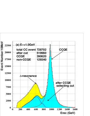
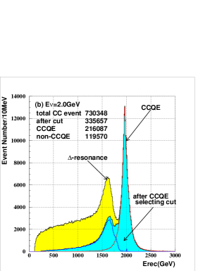
Figure 1: Reconstructed energy distributions for $\nu_{\mu}$ CC events on the water target at $E_{\nu}=1$ GeV (a) and $E_{\nu}=2$ GeV (b) according to the event generator nuance [30] when the $\mu$ momenta are measured exactly. Among $10^{6}$ generated events about 73% are CC events at both energies, which consist of CCQE events, nuclear resonance production events, and the others including deep-inelastic processes. After the CCQE selection cuts of eq. (26) are applied, the blue shaded region survive.

In a CCQE event, $\nu_{\ell}n\to\ell p$, the neutrino energy $E_{\nu}$ can be reconstructed as

$$E_{\rm rec}=\displaystyle\frac{m_{n}E_{\ell}-m_{\ell}^{2}/2-\left(m_{n}^{2}-m_{p}^{2}\right)/2}{m_{n}-E_{\ell}+p_{\ell}\cos\theta}\,,$$ (25)

in terms of the lepton energy ($E_{\ell}$), total momentum ($p_{\ell}$), and its polar angle $\theta$ about the neutrino beam direction, if a target neutron is at rest. For an anti-neutrino CCQE event, $\bar{\nu}_{\ell}p\to\bar{\ell}n$, $m_{p}$ and $m_{n}$ should be exchanged in eq. (25).

In reality, the target nucleons inside nuclei has Fermi motion of about $100$ MeV, and the measured $e$ and $\mu$ momenta have errors. Therefore, $E_{\rm rec}$ of eq. (25) is distributed around the true $E_{\nu}$, even for the CCQE processes.

The CCQE events are selected as 1-ring events in a water $\check{\rm C}$erenkov detector by the following criteria [10, 19] :

$$\mbox{{Only one charged lepton}}~{}(\ell=\mu^{\pm}\mbox{ or }e^{\pm})~{}\mbox{{with}}~{}|p_{l}|>200\mbox{{~{}MeV\,,}}$$ (26a)

$$\mbox{{No high energy}}~{}\pi^{\pm}~{}(|p_{\pi^{\pm}}|>200\mbox{{~{}MeV}})\,,$$ (26b)

$$\mbox{{No high energy}}~{}\gamma~{}(|p_{\gamma}|>30\mbox{{~{}MeV)}}\,,$$ (26c)

$$\mbox{{No}}~{}\pi^{0},~{}K_{S},~{}K_{L},~{}\mbox{{and}}~{}K^{\pm}\,.$$ (26d)

The lower limit of the total momentum in the first criterion in eq. (26a) is from the threshold of the water $\check{\rm C}$erenkov detector for $\ell=\mu$ [8]. $\pi^{\pm}$ with $|p|>200$ MeV or $\gamma$ with $|p|>30$ MeV gives rise to an additional ring. Also, $\pi^{0}$, $K_{L}$, $K_{S}$, and $K^{\pm}$ always decay inside the detector, making additional rings.

Figure 1 shows the $E_{\rm rec}$ distribution of the $\nu_{\mu}$ CC events at $E_{\nu}=1$ GeV (a) and $E_{\nu}=2$ GeV (b) on the water target, according to the event generator nuance [30]. Among the $10^{6}$ events at each energy, about 73% are CC events (the rests are NC events) which consist of CCQE events, nuclear resonance production, and the others including deep inelastic events. After the CCQE selection cuts of eq. (26) are applied, the blue shaded region survives, which consists of the CCQE events and the other events where the produced $\pi^{\pm}$ are soft. We call the non-CCQE events which survives the selection cuts of eq. (26) “resonance events”, since most of them come from single soft $\pi^{\pm}$ emission from the $\Delta$ resonance. The CCQE events and the resonance events are observed as two peaks in the reconstructed energy which are separated by about 380 MeV at $E_{\nu}\simeq 1$ GeV, rather independent of the initial $\nu_{\mu}$ energy. This is because the origin of the distance between the two peaks mainly comes from the mass difference between the nucleon and the $\Delta$ resonance, which scales as

$$\frac{(m_{\Delta}^{2}-m_{p}^{2})}{2m_{n}}\simeq 340\mbox{{~{}MeV}}$$ (27)

in eq. (25). Because the peak value of the factor, $E_{\ell}-p_{\ell}\cos\theta$, in the denominator of eq. (27) decreases from about $100$ MeV at $E_{\nu}=1$ GeV to about $50$ MeV at $E_{\nu}=2$ GeV, the difference in the peak locations decreases slightly from about $380$ MeV at $E_{\nu}=1$ GeV in Fig. 1(a) to about $360$ MeV at $E_{\nu}=2$ GeV in Fig. 1(b). The half width of the CCQE peak is about $60$ MeV, almost independent of $E_{\nu}$, because it comes from the Fermi motion of the target nucleons inside nuclei.

3.1.2 Lepton momentum resolutions

After selecting the CCQE-like events, we examine the detector resolution which further smears the $E_{\rm rec}$ distribution. We use the momentum and angular resolutions of the muon and electron at SK [8], which are shown in Table 1. For the momenta around 1 GeV, the momentum resolutions are about a few % and the angular resolutions are about a few degrees for both $\mu$ and $e$.

	${\delta p}/{p}~{}~{}(\%)$	$\delta\theta$ (degree)
$\mu$	$\left(1.7+{0.7}/{\sqrt{p\mbox{(GeV)}}}\right)$	$1.8^{\circ}$
$e$	$\left(0.6+{2.6}/{\sqrt{p\mbox{(GeV)}}}\right)$	$3.0^{\circ}$

Table 1: The momentum and angular resolution of $\mu$- and $e$-momenta at SK [8].

In Fig. 2, we show by solid curves the $E_{\rm rec}$ distributions after taking account of the $\mu^{\pm}$ momentum resolutions of Table 1, while the dotted lines show the distributions when the $\mu^{\pm}$ momenta are measured exactly, which are the boundaries of the blue shaded region in Fig. 1.

Figure 2: $E_{\rm rec}$ distribution of the CC events on the water target for monochromatic energy $\nu_{\mu}$ at $E_{\nu}=1$ GeV (a) and at $E_{\nu}=2$ GeV (b), after the CCQE selecting cuts, generated by nuance [30]. The dotted curves show the distributions when the $\mu^{\pm}$ momenta are measured exactly, the boundaries of the blue region in Fig. 1, whereas the solid lines show the distributions after the finite momentum resolution of Table 1 is taken into account.

The total width of the CCQE peak is now the sum of the effects from the Fermi motion ($\sigma_{\rm Fermi}$), the momentum resolution ($\sigma_{\delta p/p}$), and the angular resolution ($\sigma_{\delta\theta}$); it grows with $E_{\nu}$, because $\sigma_{\delta p/p}$ grows with the lepton momentum. For instance, the half width is about 60 MeV for $E_{\nu}=1$ GeV and 70 MeV for $E_{\nu}=2$ GeV. As a consequence of the energy dependence for the total width, the peak height of the CCQE events becomes lower, by about $80\%$ for $E_{\nu}=1.0$ GeV and $67\%$ for $2.0$ GeV.

The $E_{\rm rec}$ distribution for the $\nu_{e}$ CCQE events are very similar, and we do not show them separately. Small differences, due to poorer momentum resolution of electrons in Table 1, are reflected in our parameterizations in the next subsection.

3.1.3 Parameterization for the CCQE events

In this section, we present our parameterization of the $E_{\rm rec}$ distribution of the CCQE events for a given initial $\nu_{\mu}$ or $\nu_{e}$ energy $E_{\nu}$, after taking account of the $\mu$- and $e$-momentum resolutions of Table 1.

The $E_{\rm rec}$ distribution from the CCQE events can be reproduced by three Gaussians,

$$f^{\rm CCQE}_{\alpha}(E_{\rm rec};E_{\nu})=\displaystyle\frac{1}{A^{\alpha}(E_{\nu})}\sum_{n=1}^{3}r^{\alpha}_{n}(E_{\nu})\exp\left(-\displaystyle\frac{(E_{\rm rec}-E_{\nu}+{\delta}E^{\alpha}_{n}(E_{\nu}))^{2}}{2(\sigma^{\alpha}_{n}(E_{\nu}))^{2}}\right)\,,$$ (28)

where the index $\alpha$ is for $\mu$ or $e$, with $r^{\alpha}_{1}(E_{\nu})=1$. The factor $A^{\alpha}(E_{\nu})$ ensures the normalization

$$\int f^{\rm CCQE}_{\alpha}(E_{\rm rec};E_{\nu})dE_{\rm rec}=1\,.$$ (29)

The variance $\sigma^{\alpha}_{n}$, the energy shift ${\delta}E^{\alpha}_{n}$ ($n=1,2,3$), and the coefficients, $r^{\alpha}_{2}$ and $r^{\alpha}_{3}$, are parameterized as functions of the incoming neutrino energy $E_{\nu}$. These parameters depend on the neutrino species, $\nu_{\mu}$ or $\nu_{e}$, because of the mass difference in eq. (25), the difference in the momentum resolutions in Table 1, and also because of small differences in the CC cross sections at low energies [30]. Our parameterization is given in Appendix A.1, eqs. (A5)-(A10) which is valid in the region $0.3$ GeV $\leq E_{\nu}\leq$ $6.0$ GeV and $0.4$ GeV $\leq E_{\rm rec}\leq$ $5.0$ GeV for both $\nu_{\mu}$ and $\nu_{e}$. For the sake of keeping the consistency with the previous studies in ref. [23, 24, 25], those events with $E_{\rm rec}<0.4$ GeV are not used in the present analyses.

In Fig. 3, we show the $E_{\rm rec}$ distribution of the CCQE events. The solid circles show the distributions generated by nuance [30], and the histograms show our smearing functions of eq. (28). Figures. 3(a) and (b) are for $\nu_{\mu}$ and $\nu_{e}$, respectively, at $E_{\nu}=1$ GeV, and (c) and (d) are for those at $E_{\nu}=2$ GeV. The area under each distribution is normalized to unity.

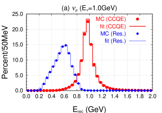
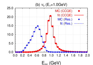
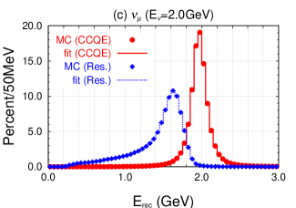
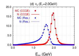
Figure 3: Normalized $E_{\rm rec}$ distribution of the CCQE events (solid circles) and the resonance events (solid diamonds) after the CCQE selection cuts of eq. (26) and the momentum resolutions for $\mu$ and $e$ in Table 1 are applied. The events are generated by nuance [30]. The solid line shows our parameterization for the CCQE events and the dotted line is for the resonance events: (a) $\nu_{\mu}$ and (b) $\nu_{e}$ at $E_{\nu}=1$ GeV; (c) $\nu_{\mu}$ and (d) $\nu_{e}$ at $E_{\nu}=2$ GeV.

3.1.4 Nuclear resonance contributions

The $E_{\rm rec}$ distribution of the non-CCQE events which pass the CCQE selection cuts of eq. (26) can also be parameterized. Most of them come from the $\Delta$ resonance production, and the resonance peak in the $E_{\rm rec}$ distribution is observed in Figs. 1 and 2. For $E_{\nu}\leq 1.2$ GeV, 3 Gaussians suffice to reproduce the $E_{\rm rec}$ distributions generated by nuance [30];

$$f^{\rm res}_{\alpha}(E_{\rm rec};E_{\nu}\leq 1.2\mbox{GeV})=\displaystyle\frac{1}{\hat{A}^{\alpha}(E_{\nu})}\sum_{n=1}^{3}\hat{r}^{\alpha}_{n}(E_{\nu})\exp\left(-\displaystyle\frac{(E_{\rm rec}-E_{\nu}+\delta\hat{E}_{n}^{\alpha}(E_{\nu}))^{2}}{2(\hat{\sigma}_{n}^{\alpha}(E_{\nu}))^{2}}\right)\,,$$ (30)

while at high energies ($E_{\nu}>1.2$ GeV), we need 4 Gaussians, because the number of contributing resonances grows with $E_{\nu}$;

$$f^{\rm res}_{\alpha}(E_{\rm rec};E_{\nu}>1.2\mbox{GeV})=\displaystyle\frac{1}{\tilde{A}^{\alpha}(E_{\nu})}\sum_{n=1}^{4}\tilde{r}^{\alpha}_{n}(E_{\nu})\exp\left(-\displaystyle\frac{(E_{\rm rec}-E_{\nu}+{\delta}\tilde{E}^{\alpha}_{n}(E_{\nu}))^{2}}{2(\tilde{\sigma}_{n}^{\alpha}(E_{\nu}))^{2}}\right)\,.$$ (31)

Around $E_{\nu}\sim 1.2$ GeV, both parameterizations are valid. Here again $\alpha$ is $\mu$ or $e$, $\hat{r}^{\mu,e}_{1}(E_{\nu})=\tilde{r}^{\mu,e}_{1}(E_{\nu})=1$, and the factors $\hat{A}(E_{\nu})$ and $\tilde{A}(E_{\nu})$ assure that the smearing functions are normalized to 1 as in eq. (29). The variances $\hat{\sigma}^{\alpha}_{n}$ and $\tilde{\sigma}^{\alpha}_{n}$, the energy shifts ${\delta}\hat{E}^{\alpha}_{n}$, ${\delta}\tilde{E}^{\alpha}_{n}$, and the relative normalization factors $\hat{r}^{\alpha}_{n}$ and $\tilde{r}^{\alpha}_{n}$ ($n\neq 1$) are all parameterized as functions of the incoming energy $E_{\nu}$, which are given in Appendix A.2. The shape of the $E_{\rm rec}$ distribution for the “resonance” events are also shown in Fig. 3. The solid diamonds show the distribution of non-CCQE events generated by nuance [30] after the CCQE selection cuts of eq. (26) and the momentum resolutions of Table 1 are applied. The dotted histograms show our smearing functions, eqs. (30) and (31).

3.2 NC events

The key observation of ref. [23, 24] for the T2KK proposal is that it is advantageous to observe the first oscillation maximum ($|\Delta_{13}|\sim\pi$) at two vastly different baseline lengths, $L=295$ Km at SK and $L\simeq 1000$ km in Korea. Higher energy neutrino beam, or small off-axis angle, is hence desired for the far detector in Korea. However, the use of high energy (broad band) beam gives rise to a serious background for the $\nu_{\mu}\to\nu_{e}$ oscillation signal. The single $\pi^{0}$ production via the neutral current (NC), whose cross section grows with $E_{\nu}$, cannot always be distinguished from the $\nu_{\mu}\to\nu_{e}$ signal in a water $\check{\rm C}$erenkov detector. In this subsection, we study the NC $\pi^{0}$ production background in detail and estimate its $E_{\rm rec}$ distribution by using the momentum distribution of misidentified $\pi^{0}$’s.

3.2.1 Event selection

We simulate the NC $\pi^{0}$ production background as follows. By using the neutrino flux of the T2K beam at various off-axis angles between $0.0^{\circ}$(on-axis) and $3.0^{\circ}$, and by using the total cross section $\sigma_{\rm tot}^{\alpha}$ ($\alpha=\nu_{\mu},\bar{\nu}_{\mu},\nu_{e},$ and $\bar{\nu}_{e}$) off the water target [30], both CC and NC events are generated by nuance [30] for a water $\check{\rm C}$erenkov detector of 100 kton fiducial volume at $L=1000$ km, with $5\times 10^{21}$ POT. All the generated events are then confronted against the following selection criteria :

No charged leptons. (32a)

$$\mbox{{Only one}}~{}\pi^{0}\,.$$ (32b)

$$\mbox{{No high energy}}~{}\pi^{\pm}~{}(|p_{\pi^{\pm}}|<200\mbox{{~{}MeV.}})$$ (32c)

$$\mbox{{No high energy}}~{}\gamma~{}(|p_{\gamma}|<30\mbox{{~{}MeV.}})$$ (32d)

$$\mbox{{No}}~{}K_{L},~{}K_{S},~{}K^{\pm}.$$ (32e)

The first condition, eq. (32a), selects NC events, and the others eliminate multi-ring events. The $\pi^{0}$ momentum distribution after the above cuts is shown in Fig. 4(a) for various off-axis beams. We find that the number of single $\pi^{0}$ events grows with decreasing off-axis angle, especially for the angles below $2.0^{\circ}$ which have been envisaged in ref. [23, 24, 25] as an optimal choice for the far detector in Korea.

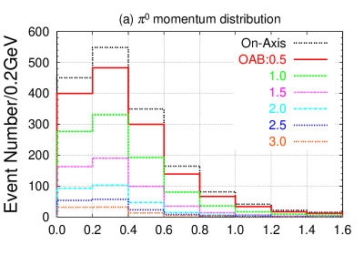
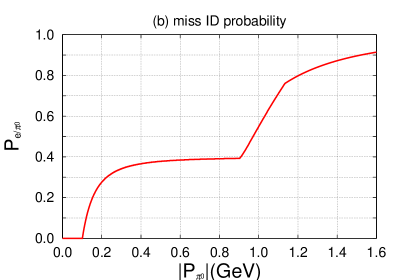
Figure 4: (a): The $\pi^{0}$ momentum distribution of the single $\pi^{0}$ NC events selected by the criteria, eq. (32), at various off-axis angles. The event numbers are obtained for a 100 kton water target at $L=1000$ km with $5\times 10^{21}$POT, according to nuance [30]. (b): Probability that a $\pi^{0}$ cannot be distinguished from $e^{\pm}$, according to eq. (36). The common horizontal axis measures the $\pi^{0}$ momentum.

3.2.2 $\pi^{0}$ - $e^{\pm}$ misidentification probability

Figure. 4(a) shows that there are many single-$\pi^{0}$ events from the NC interactions, especially for smaller off-axis angles. Some of them become backgrounds of the $\nu_{\mu}\to\nu_{e}$ oscillation signal, because the two photons from $\pi^{0}$ are not always resolved by a water $\check{\rm C}$erenkov detector. When one of the two photons is much softer than the other, the soft photon dose not give a clear ring, resulting in a single-ring ($e$-like) event. In addition, when the photons have a small opening angle the overlapping rings cannot always be resolved.

We therefore parameterize the probability of misidentifying $\pi^{0}$ as an $e^{\pm}$ in terms of the energy ratio and the opening angle of the two photons in the laboratory frame. The energy fraction of the softer photon in the laboratory frame

$$x=\displaystyle\frac{E_{2}}{E_{1}+E_{2}}~{}~{}~{}(E_{2}<E_{1})$$ (33)

can be expressed as

$$x=\displaystyle\frac{1}{2}\left(1-\beta\cos\hat{\theta}\right)\,,~{}~{}~{}~{}~{}~{}$$ (34)

in terms of the smaller polar angle ($\cos\hat{\theta}>0$) of the photon momentum in the $\pi^{0}$ rest frame about the polar axis along the $\pi^{0}$ velocity ($\beta$) in the laboratory frame. The opening angle between the two photons in the laboratory frame is then

$$\cos\theta_{\gamma\gamma}=1-\displaystyle\frac{1-\beta^{2}}{2x\left(1-x\right)}\,.$$ (35)

It is clear from eqs. (34) and (35) that when the $\pi^{0}$ momentum is relativistic ($\beta\to 1$) either one of the photons becomes soft $(x\ll 1)$ around $\cos\hat{\theta}\sim 1$, or the two photons become collinear, $\cos\theta_{\gamma\gamma}\sim 1$.

By using the energy fraction $x$ and $\cos\theta_{\gamma\gamma}$, the $\pi^{0}$-$e^{\pm}$ misidentification probability can be parameterized as

$$P_{e/\pi^{0}}(|p_{\pi^{0}}|)=\int_{0}^{1}\left[\Theta(x^{0}-x)+\Theta(x-x^{0})\Theta(\cos\theta_{\gamma\gamma}-\cos\theta_{\gamma\gamma}^{0})f(x,\cos\theta_{\gamma\gamma})\right]d\cos\hat{\theta}\,,$$ (36)

where $\Theta(x)$ is the step function. The first step function in the r.h.s. tells that the $\pi^{0}$ is misidentified as an $e^{\pm}$ when the energy fraction $x$ of the soft photon is smaller than $x^{0}$. When both photons are hard $(x^{0}<x<0.5)$, it is still misidentified as an $e^{\pm}$ when $\cos\theta_{\gamma\gamma}>\cos\theta_{\gamma\gamma}^{0}$. We introduce a fudge factor

$$f(x,\cos\theta_{\gamma\gamma})=1.0-\left(\displaystyle\frac{x-x^{0}}{0.5-x^{0}}\right)^{1/2}\left(\displaystyle\frac{1.0-\cos\theta_{\gamma\gamma}}{1.0-\cos\theta_{\gamma\gamma}^{0}}\right)^{3/2}\,,$$ (37)

in order to take account of detector performance. We show in Fig. 4(b) the $\pi^{0}$-$e^{\pm}$ misidentification probability, $P_{e/\pi^{0}}(|p_{\pi^{0}}|)$, of eq. (36) for $x^{0}=0.2$ and $\theta^{0}=17^{\circ}$, which reproduces qualitatively the typical performance of water $\check{\rm C}$erenkov detectors. The leadoff energy, $|p_{\pi^{0}}|=0.1$ GeV, and the height of the plateau, $P_{e/\pi^{0}}=0.4$, are dictated by the first step function in eq. (36), which tells that the two photons are not resolved when the softer photon has an energy fraction less than 0.2. The second term in eq. (36) determines the kink structure around $|p_{\pi^{0}}|=0.9$ and $11.0$ GeV, as well the asymptotic behavior at high $\pi^{0}$ momentum.

The number of the $e$-like events from the $\pi^{0}$ background can now be calculated as the product of the $\pi^{0}$ event number in Fig. 4(a) and the probability $P_{e/\pi^{0}}(|p_{\pi^{0}}|)$ in Fig. 4(b). The reconstructed energy $E_{\rm rec}$ of each $\pi^{0}$ background event is calculated from the $\pi^{0}$ energy and the scattering angle by assuming the electron mass.

3.3 The event numbers

We calculate the numbers of $\nu_{\mu}$ and $\nu_{e}$ CC events from the primary and the secondary beam in the $i$-th energy bin, $E_{\rm rec}^{i}<E<E_{\rm rec}^{i+1}$, as

$$N_{\beta,D}^{i,X}(\nu_{\alpha})=MN_{A}\int_{E_{\rm rec}^{i}}^{E_{\rm rec}^{i+1}}\!\!\!\!\!dE_{\rm rec}\int_{0}^{\infty}dE_{\nu}\left[\Phi_{\nu_{\alpha}}^{D}(E_{\nu})~{}P_{\nu_{\alpha}\to\nu_{\beta}}^{D}(E_{\nu})~{}\hat{\sigma}_{\beta}^{X}(E_{\nu})~{}f^{X}_{\beta}(E_{\rm rec};E_{\nu})\right]\,,$$ (38)

where $E_{\rm rec}^{i}=0.2{\rm GeV}\times i$. Here $M$ is the detector mass (g), $N_{A}=6.017\times 10^{23}$ (mol^-1) is the Avogadro number, $\Phi_{\nu_{\alpha}}$ is the $\nu_{\alpha}$ flux ($\nu_{\alpha}=\nu_{\mu},\bar{\nu}_{\mu},\nu_{e},\bar{\nu}_{e}$) of the T2K $\nu_{\mu}$-beam [38], which is dominated by $\nu_{\mu}$ but has secondary $\bar{\nu}_{\mu}$, $\nu_{e}$, $\bar{\nu}_{e}$ components. $P_{\nu_{\alpha}\to\nu_{\beta}}$ denotes the neutrino oscillation probability for $\nu_{\mu},\nu_{e}\to\nu_{\mu},\nu_{e}$ or $\bar{\nu}_{\mu},\bar{\nu}_{e}\to\bar{\nu}_{\mu},\bar{\nu}_{e}$, including the matter effect. $\hat{\sigma}_{\beta}^{X}(E_{\nu})~{}$ is the cross section of the $\nu_{\beta}$ CC events for the CCQE process ($X=$ CCQE) and the non-CCQE processes ($X=$ Res) per nucleon in water. The last term of eq. (38), $f^{X}_{\beta}(E_{\rm rec};E_{\nu})$ is the smearing function of eq. (28) for the CCQE events, and that of eqs. (30) and (31) for the “resonance” events. The index $D$ tells the detector location; the baseline length for $D=$ SK is 295 km and that for the far detector $D=$ Kr is chosen between $L=1000$ km and $1200$ km.

The effective CCQE cross section per nucleon is slightly smaller than the naive cross section at high energies;

$${\hat{\sigma}_{\beta}^{\rm CCQE}(E_{\nu})}={{\sigma}_{\beta}^{\rm CCQE}(E_{\nu})}\times\left\{\begin{array}[]{ll}1.0\,,&(\mbox{for }E_{\nu}\mbox{[GeV]}<0.9)\\ 1.0-0.054\left(\displaystyle\frac{E_{\nu}-0.90}{E_{\nu}-0.26}\right)\,,&(\mbox{for }E_{\nu}\mbox{[GeV]}>0.9)\end{array}\right.$$ (39)

because of occasional emission of $\pi^{0}$ or $\gamma$ from the oxygen nuclei. As for the naive CCQE cross section per nucleon, ${\sigma}_{\beta}^{\rm CCQE}(E_{\nu})$ for $\nu_{\beta}$ $(\nu_{\beta}=\nu_{\mu},\bar{\nu}_{\mu},\nu_{e},\bar{\nu}_{e})$ in water, we use the estimates of ref. [39] throughout the present analysis. The reduction factor in eq. (39) is our parameterization of the outputs of nuance [30].

The effective resonance event cross section $\hat{\sigma}_{\beta}^{\rm Res}(E_{\nu})$ is the total cross section of all the non-CCQE CC events that satisfy the CCQE selection criteria of eq. (26). They are slightly different between $\nu_{\mu}$ and $\nu_{e}$ CC events, and we find that the following parameterizations

$$\hat{\sigma}_{e}^{\rm Res}(E_{\nu})\!\!\! = \!\!\!{\sigma}_{e}^{\rm CCQE}(E_{\nu})\left(0.789+0.00738\log E_{\nu}-\displaystyle\frac{0.455}{E_{\nu}}\right)\,,~{}(\mbox{ for }E_{\nu}\mbox{[GeV]}>0.51)\,,$$ (40a)

$$\hat{\sigma}_{\mu}^{\rm Res}(E_{\nu})\!\!\! = \!\!\!{\sigma}_{\mu}^{\rm CCQE}(E_{\nu})\left(0.810+0.00738\log E_{\nu}-\displaystyle\frac{0.436}{E_{\nu}}\right)\,,~{}(\mbox{ for }E_{\nu}\mbox{[GeV]}>0.54)\,,~{}~{}~{}~{}~{}$$ (40b)

reproduce well the results of nuance [30]. The gradual increase of the non-CCQE rates with $E_{\nu}$ reflects the growth of the number of contributing resonances and deep-inelastic events at high energies.

Both the fudge factors in eqs. (39) and (40) and the smearing functions eqs. (28), (30), and (31), are obtained for $\nu_{\mu}$ and $\nu_{e}$ CC events. They can be slightly different for $\bar{\nu}_{\mu}$ and $\bar{\nu}_{e}$ CC events because of isospin breaking ($m_{p}\neq m_{n}$, $m_{\Delta^{+}}\neq m_{\Delta^{0}}$, etc. ) and the presence of isolated protons in a water molecule. However, because the secondary anti-neutrino fluxes are small, we use the same fudge factors and the smearing functions for anti-neutrinos, simply by replacing the CCQE cross sections by those of anti-neutrinos.

The total number of the signal CC events in each bin is now expressed as

$$N_{\alpha,D}^{i,{\rm CC}}=\varepsilon_{\alpha}\sum_{X={\rm CCQE},{\rm Res}}\left[N_{\alpha,D}^{i,X}(\nu_{\mu})+N_{\alpha,D}^{i,X}(\nu_{e})+N_{\bar{\alpha},D}^{i,X}(\bar{\nu}_{\mu})+N_{\bar{\alpha},D}^{i,X}(\bar{\nu}_{e})\right]\,,$$ (41)

for $\alpha=\mu$ and $e$, if there are no background. Here $\varepsilon_{\mu}$ and $\varepsilon_{e}$ are the detection efficiencies for observing the $\mu^{\pm}$ or $e^{\pm}$ signal, respectively. In actual experiments, there is a small probability of a percent level that a $\mu^{\pm}$ is misidentified as an $e^{\pm}$ signal, $P_{e/\mu}$, and also the reciprocal probability, $P_{\mu/e}$, of taking $e^{\pm}$ as $\mu^{\pm}$. In addition, significant fraction of single $\pi^{0}$ production events via NC cannot be distinguished from the $e^{\pm}$ CCQE signal as explained in the previous subsection. After adding those backgrounds the total number of a observed events can be expressed as

$$N_{\mu,D}^{i} = (1-P_{e/\mu})N_{\mu,D}^{i,{\rm CC}}+P_{\mu/e}\cdot N_{e,D}^{i,{\rm CC}}\,,$$ (42a)

$$N_{e,D}^{i} = P_{e/\mu}\cdot N_{\mu,D}^{i,{\rm CC}}+(1-P_{\mu/e})N_{e,D}^{i,{\rm CC}}+N_{\pi^{0},D}^{i,{\rm NC}}\,,$$ (42b)

where $N_{\pi^{0},D}^{i,{\rm NC}}$ is the event numbers from the NC $\pi^{0}$ background in the $i$-th bin.

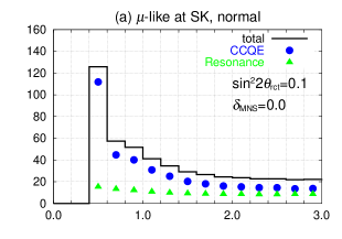
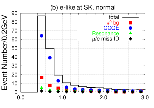
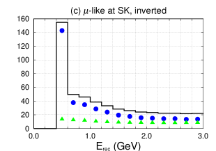
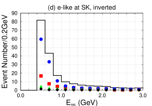
Figure 5: Typical numbers of the $\mu$-like events, (a) and (c), and $e$-like events, (b) and (d), for the $3.0^{\circ}$ OAB at SK with $5\times 10^{21}$POT. (a) and (b) are for the normal hierarchy, and (c) and (d) are for the inverted hierarchy. The histograms gives the total event numbers, the circles and the triangles are the CCQE and the “resonance” event numbers, respectively. The squares and diamonds in (a) and (c) stand for the background event numbers from the misidentified $\pi^{0}$ and $\mu^{\pm}$, respectively. The inputs are listed in eqs. (43)-(45). We show only those events with $E_{\rm rec}>0.4$ GeV used in our analysis.

In Fig. 5(a) and (b), typical $e$- and $\mu$-like event numbers with $5\times 10^{21}$POT for the $3.0^{\circ}$ OAB at SK is shown, when the normal hierarchy is assumed. Figures 5(c) and (d) are for the inverted hierarchy. The histogram gives the total event numbers, and the circles and the triangles give the CCQE and non-CCQE “resonance” event numbers, respectively. The squares and the diamonds in (b) and (d) show the background event numbers from the misidentified $\pi^{0}$ and $\mu^{\pm}$, respectively. Events with $E_{\rm rec}<0.4$ GeV $(i=0$ and $1)$ are not shown because we do not use them in our analysis.

The input values of the neutrino mass and mixing parameters adopted for Fig. 5 are

$$\left|\delta m^{2}_{13}\right| = 2.5\times 10^{-3}\mbox{{eV${}^{2}$}}\,,\hskip 21.52771pt\sin^{2}\theta_{\scriptscriptstyle{\rm ATM}}=0.5\,,$$ (43a)

$$\delta m^{2}_{12} = 8.2\times 10^{-5}\mbox{{eV${}^{2}$}}\,,\hskip 21.52771pt\sin^{2}2\theta_{\scriptscriptstyle{\rm SOL}}=0.83\,,$$ (43b)

$$\sin^{2}2\theta_{\scriptscriptstyle{\rm RCT}} = 0.10\,,\hskip 21.52771pt\delta_{\scriptscriptstyle{\rm MNS}}=0^{\circ}\,.$$ (43c)

Although the central values of the most recent measurements in eqs. (2) and (4) are slightly different, we use the above values in order to compare our results quantitatively with those of the previous studies in ref. [23, 24].

The matter density along the baseline between J-PARC and SK, and that between J-PARC and the far detector in Korea are taken as

$$\rho_{\rm SK} = 2.6\mbox{{g/cm${}^{3}$ for SK}}\,,$$ (44a)

$$\rho_{\rm Kr} = 3.0\mbox{{g/cm${}^{3}$ for Korea}}\,.$$ (44b)

These average matter densities along the baseline are obtained [34] from the recent geophysical measurements [40, 41] which have typical errors of about $6\%$. The value for the T2K baseline eq. (44a) is slightly lower than $2.8$g/cm³ quoted in ref. [19], because of the “Fossa Magna” along the baseline, in which the average density is as low as $2.5$g/cm³. The average matter density along the baseline for the far detector in Korea depends slightly on the baseline length between $L=1000$ km and $1200$ km, because it goes through the upper mantle. Those details as well as the impacts of the matter profile along the baseline will be reported elsewhere [34].

Finally, the efficiencies for detecting $\mu^{\pm}$ and $e^{\pm}$ sinal events in eq. (41) and the probability of misidentifying $\mu^{\pm}$ as $e^{\pm}$ ($P_{e/\mu}$) and that of misidentifying $e^{\pm}$ as $\mu^{\pm}$ ($P_{\mu/e}$) in eq. (42) are respectively,

$$\varepsilon_{\mu} = 100\%\,,\hskip 21.52771pt\varepsilon_{e}=90\%\,,$$ (45a)

$$P_{e/\mu} = 1\%\,,\hskip 30.1388ptP_{\mu/e}=0\%\,.$$ (45b)

Hereafter we set $P_{\mu/e}=0$ for simplicity, because $P_{\mu/e}\sim 1\%$ does not affect our results significantly due to the smallness of the expected number of $e^{\pm}$ events.

The $\nu_{\mu}$ survival probability is less than $40\%$ in the region $0.4$ GeV $<E_{\nu}<1.0$ GeV, because of the oscillation dip for $P_{\nu_{\mu}\to\nu_{\mu}}$ at $E_{\nu}\simeq 0.6$ GeV. Nevertheless, we expect many CCQE events with $E_{\rm rec}<1.0$ GeV in Fig. 5(a) and (c) due to the high intensity of the $\nu_{\mu}$ flux at $3.0^{\circ}$ off-axis angle, which has a peak at $E_{\nu}\simeq 0.5$ GeV. It catches our eyes that the $\mu$-like event rate in the first bin (0.4 GeV$\leq E_{\rm rec}\leq$0.6 GeV) is significantly larger for the inverted hierarchy than for the normal hierarchy. This is because the oscillation phase shift, the factor $B^{\mu}$ in eqs. (21a) and (23b), is negative for the parameters of eq. (43) so that the location of the dip occurs at slightly higher $E_{\nu}$ for the inverted hierarchy. Such small difference in the dip location between the two hierarchies, however, can be compensated by a small shift in $|\delta m^{2}_{13}|$ of several percent order. This in turn tells that $|\delta m^{2}_{13}|$ cannot be measured beyond the accuracy of several percent unless the mass hierarchy pattern is determined; see discussions in section 5.4 for more details.

Typical $e$-like events at SK are shown in Figs. 5(b) and (d). The CCQE events dominate the $e$-like events for both mass hierarchies. Because there is little high energy tail for the $3.0^{\circ}$ OAB and the probability of misidentifying $\pi^{0}$ as $e^{\pm}$ is not large at $E_{\nu}<1.0$ GeV, as can be seen from Figs. 4(a) and (b), respectively, the $\pi^{0}$ background events given by the squares do not dominate over the CCQE signal events. Nevertheless, they consist of about $20\%$ of the total number of $e$-like events in the first three bins of $E_{\nu}<1.0$ GeV. Quantitative estimate of the $\pi^{0}$ background should hence be essential to measure the $\nu_{\mu}\to\nu_{e}$ transition probability with confidence.

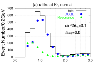
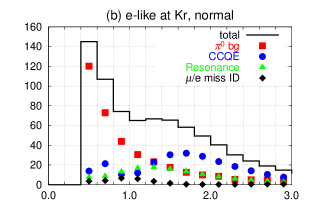
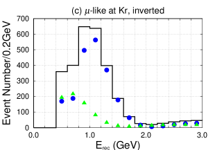
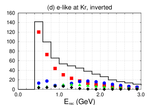
Figure 6: The same as Fig. 5, but for the $0.5^{\circ}$ OAB at $L=1000$ km with a 100 kton water $\check{\rm C}$erenkov detector.

In Fig. 6, we show the $E_{\rm rec}$ distributions of the $\mu$-like and $e$-like events expected for a 100 kton far detector at $L=1000$ km and with the $0.5^{\circ}$ OAB, for exactly the same model parameters of eq. (43) and the systematics of eq. (45), but with the average matter density of eq. (44b).

The $E_{\rm rec}$ distributions of the $\mu$-like events are shown for the normal and inverted hierarchy in Figs. 6(a) and (b), respectively, where little dependence on the mass hierarchy pattern can be observed. The $\nu_{\mu}\to\nu_{\mu}$ oscillation dip at $E_{\nu}\sim 2.0$ GeV is clearly seen in both cases, despite the contribution from the non-CCQE “resonance” events shown by the triangles, which has a dip at lower $E_{\rm rec}$.

What is most surprising in Fig. 6 is the overwhelmingly large contribution of the $\pi^{0}$ background events, shown by the squares, in the $e$-like event distributions, both in (b) and (d), respectively, for the normal and the inverted hierarchies. They dominate the CCQE signal at low $E_{\rm rec}$, $E_{\rm rec}<1.4$ GeV for the normal hierarchy and $E_{\rm rec}<1.6$ GeV for the inverted hierarchy. This is essentially because of the hard energy (broad band) spectrum of the $0.5^{\circ}$ OAB, which gives rise to copious production of single $\pi^{0}$ events via the NC. Nevertheless, the CCQE event numbers supersede the $\pi^{0}$ background at high $E_{\rm rec}$, $E_{\rm rec}>1.4$ GeV for the normal hierarchy, and $E_{\rm rec}$, $E_{\rm rec}>1.6$ GeV for the inverted hierarchy. The significant difference in the $E_{\rm rec}$ distributions of the $e$-like events expected at a far detector, between Figs. 6(b) and (d), in contrast to the similarity of the corresponding distributions at SK, between Figs. 5(b) and (d), may allow us to determine the neutrino mass hierarchy even in the presence of the $\pi^{0}$ background, since the $\pi^{0}$ background due to the NC events do not depend on the mass hierarchy. The non-CCQE “resonance” events, shown by the triangle, behave similarly to the CCQE signal events; the number of events is enhanced for the normal hierarchy and suppressed for the inverted hierarchy. Therefore, we expect that the contribution from the “resonance” events will enhance the sensitivity of the T2KK experiment to the mass hierarchy.

4 Analysis Method

In order to quantify the physics potential of the T2KK neutrino oscillation experiment, we introduce a $\chi^{2}$ function

$$\chi^{2}\equiv\chi^{2}_{\rm SK}+\chi^{2}_{\rm Kr}+\chi^{2}_{\rm sys}+\chi^{2}_{\rm para}\,,$$ (46)

which measures the sensitivity of the expected measurements on the physics parameters such as the neutrino mass hierarchy, $\sin^{2}2\theta_{\scriptscriptstyle{\rm RCT}}$ and $\delta_{\scriptscriptstyle{\rm MNS}}$, in the presence of statistical errors as well as various systematic errors including the uncertainties in the other parameters of the three neutrino model.

The first two terms in eq. (46), $\chi^{2}_{\rm SK}$ and $\chi^{2}_{\rm Kr}$, respectively, measure the constraints from the measurements at SK and a far detector in Korea;

$$\chi^{2}_{D}=\sum_{i}\left\{\left(\displaystyle\frac{(N_{\mu,D}^{i})^{\rm fit}-(N_{\mu,D}^{i})^{\rm input}}{\sqrt{(N^{i}_{\mu,D})^{\rm input}}}\right)^{2}+\left(\displaystyle\frac{(N_{e,D}^{i})^{\rm fit}-(N_{e,D}^{i})^{\rm input}}{\sqrt{(N^{i}_{e,D})^{\rm input}}}\right)^{2}\right\}\,,(D={\rm SK,Kr})\,.$$ (47)

Here $(N_{\mu,D}^{i})^{\rm input}$ and $(N_{e,D}^{i})^{\rm input}$ denotes the $\mu$-like and $e$-like event numbers, respectively, at SK ($D=$ SK) and at a far detector in Korea ($D=$ Kr), in the $i$-th bin of $E_{\rm rec}$ calculated as in eq. (38)-(42), and its square root gives the statistical error. The summation is over all bins from $0.4$ GeV to $5.0$ GeV at both detectors for $N_{\mu}$, $0.4$ GeV to $1.2$ GeV at SK, and $0.4$ GeV to $2.8$ GeV at Korea for $N_{e}$. In order to compare our results quantitatively with those of the previous studies in ref. [23, 24, 25], we use the same input values of the neutrino model parameters, as in eq. (43), when calculating the expected number of events in each bin.

The event numbers for the fit, $(N_{\mu,D}^{i})^{\rm fit}$ and $(N_{e,D}^{i})^{\rm fit}$ are calculated as

$$\left(N_{\mu,D}^{i}\right)^{\rm fit}\!\!\! = \!\!\!f_{\rm V}^{D}\left[\left(1-P_{e/\mu}\right)\sum_{X,\alpha,\beta}\varepsilon_{\mu}f_{\nu_{\alpha}}^{D}f_{\beta}^{X}N_{\mu,D}^{i,X}(\nu_{\alpha})\right]\,,$$ (48a)

$$\left(N_{e,D}^{i}\right)^{\rm fit}\!\!\! = \!\!\!f_{\rm V}^{D}\left[\sum_{X,\alpha,\beta}\left\{\varepsilon_{e}f_{\nu_{\alpha}}^{D}f_{\beta}^{X}N_{e,D}^{i,X}(\nu_{\alpha})+P_{e/\mu}f_{\nu_{\alpha}}^{D}f_{\beta}^{X}N_{\mu,D}^{i,X}(\nu_{\alpha})\right\}+f_{\nu_{\mu}}^{D}f_{\pi^{0}}N^{i,NC}_{\pi^{0},D}\right]\,,~{}~{}~{}~{}~{}~{}~{}~{}$$ (48b)

where the initial neutrino flavor, $\nu_{\mu}$, $\bar{\nu}_{\mu}$, $\nu_{e}$, $\bar{\nu}_{e}$, are denoted as $\nu_{\alpha}$ with $\alpha=\mu$, $\bar{\mu}$, $e$, $\bar{e}$, respectively, and the superscript $X$ denotes the event type, $X=$ CCQE for the signal, or $X=$ Res for the non-CCQE “resonance” events that pass the CCQE selection criteria of eq. (26). The subscript $\beta$ distinguishes neutrinos ($\beta=\nu$ for $\nu_{\mu}$ or $\nu_{e}$) and anti-neutrino ($\beta=\bar{\nu}$ for $\nu_{\mu}$ or $\nu_{e}$), while $D=$ SK or $D=$ Kr as in eq. (47). We introduce 17 normalization factors whose deviation from unity measures systematic uncertainties, 15 of which appear explicitly in eq. (48); $f_{V}^{D}$ for the fiducial volume and $f_{\nu_{\alpha}}^{D}$ for the initial neutrino flux at $D=$ SK and $D=$ Kr, $f_{\beta}^{X}$ for the CC cross section of $X=$ CCQE or $X=$ Res with neutrino ($\beta=\nu$) or anti-neutrino ($\beta=\bar{\nu}$), and $f_{\pi^{0}}$ for the NC cross section of producing the single $\pi^{0}$ background. In addition the factor $f_{\rho}^{D}$ takes account of the uncertainty in the average matter density along the baseline between J-PARC and SK ($D=$ SK) or Korea ($D=$ Kr), which appear in the computation of the oscillation probability $P_{\nu_{\alpha}\to\nu_{\beta}}$ by modifying the matter density as

$$\rho_{D}^{\rm fit} = f^{D}_{\rho}\,\rho^{\rm input}_{D}\,,\hskip 21.52771pt(D={\rm SK,~{}Kr})\,.$$ (49)

By using the above 17 normalization factors, the detection efficiencies ($\varepsilon_{e}$ and $\varepsilon_{\mu}$) and the $\mu$-to-$e$ misidentification probability ($P_{e/\mu}$), we estimate the systematic effects as follows;

$$\chi^{2}_{\rm sys} = \sum_{D={\rm SK,~{}Kr}}\left\{\left(\displaystyle\frac{f^{D}_{\rm V}-1}{0.03}\right)^{2}+\left(\displaystyle\frac{f^{D}_{\rho}-1}{0.06}\right)^{2}+\sum_{\alpha=e,\bar{e},\mu,\bar{\mu}}\left(\displaystyle\frac{f_{\nu_{\alpha}}^{D}-1}{0.03}\right)^{2}\right\}$$ (50)

$$+\sum_{\beta=\nu,\bar{\nu}}\left\{\left(\displaystyle\frac{f^{\rm CCQE}_{\beta}-1}{0.03}\right)^{2}+\left(\displaystyle\frac{f^{\rm Res}_{\beta}-1}{0.20}\right)^{2}\right\}+\left(\displaystyle\frac{f_{\pi^{0}}-1}{0.50}\right)^{2}$$

$$+\left(\displaystyle\frac{\varepsilon_{e}-0.9}{0.05}\right)^{2}+\left(\displaystyle\frac{\varepsilon_{\mu}-1}{0.01}\right)^{2}+\left(\displaystyle\frac{P_{e/\mu}-0.01}{0.01}\right)^{2}\,.~{}~{}$$

All the errors in the first row of eq. (50) depend on the detector and its location, $D=$ SK and $D=$ Kr. The first term is the uncertainty of the fiducial volume, for which we assign $3\%$ error independently for SK ($f_{\rm V}^{\rm SK}$) and a far detector in Korea ($f_{\rm V}^{\rm Kr}$). The second one is for the matter density uncertainties along the T2K ($f^{\rm SK}_{\rho}$) and the Tokai-to-Korea ($f^{\rm Kr}_{\rho}$) baseline. The dominant source of the error in the matter density arises when the sound velocity data are translated into the matter density [34, 42], and we assign 6$\%$ error independently for each baseline. The last term of the first row is for the overall normalization of each neutrino flux, which are taken independently for each neutrino species and the detector location. This is a conservative estimate, since it is likely that all the flux normalization errors are positively correlated. The second row gives the uncertainty in the cross sections. Because the CCQE cross section for $\nu_{e}$ and $\nu_{\mu}$ are expected to be very similar theoretically, we assign a common overall error of $3\%$ for $\nu_{e}$ and $\nu_{\mu}$ ($f_{\nu}^{\rm CCQE}$) and an independent $3\%$ error for $\bar{\nu}_{e}$ and $\bar{\nu}_{\mu}$ ($f_{\bar{\nu}}^{\rm CCQE}$). For non-CCQE “resonance” events ($f_{\beta}^{\rm Res}$), we assume $20\%$ error for $\beta=\nu$ and $\beta=\bar{\nu}$ independently, since it depends not only on the single $\pi$ production cross section but also on the momentum distribution and the detector performance. We allow $50\%$ error for the NC cross section of producing single $\pi^{0}$ background ($f_{\pi^{0}}$), since it takes account of the uncertainty in the $\pi^{0}$-to-$e$ misidentification probability ($P_{\pi^{0}/e}$). The systematic errors in the last row of eq. (50) account for the performance of a water $\check{\rm C}$erenkov detector. The first and the second terms denote the uncertainty of the detection efficiency for $e$- and $\mu$-like events, respectively. In this analysis, we adopt $\delta\varepsilon_{e}=5\%$ and $\delta\varepsilon_{\mu}=1\%$, which are taken common for SK and a far detector in Korea. The last one is the probability of misidentifying a $\mu$-event as an $e$-event, for which a common error of 1$\%$ is assumed. In total, we adopt 20 parameters in simulating the systematic errors.

Finally, $\chi^{2}_{\rm para}$ accounts for external constraints on the model parameters:

$$\chi^{2}_{\rm para} = \left(\displaystyle\frac{\left(\delta m^{2}_{12}\right)^{\rm fit}-8.2\times 10^{-5}\mbox{{eV}${}^{2}$}}{0.6\times 10^{-5}}\right)^{2}+\left(\displaystyle\frac{\sin^{2}2\theta_{\scriptscriptstyle{\rm SOL}}^{\rm fit}-0.83}{0.07}\right)^{2}$$ (51)

$$+\left(\displaystyle\frac{\sin^{2}2\theta_{\scriptscriptstyle{\rm RCT}}^{\rm fit}-\sin^{2}2\theta_{\scriptscriptstyle{\rm RCT}}^{\rm input}}{0.01}\right)^{2}\,.$$

Although the errors of the smaller mass-squared difference and the solar mixing angle in eq. (51) are somewhat larger than their most recent values in eq. (4), we stick to the above estimates in order to compare our results quantitatively with those of the previous studies in ref. [23, 24, 25]. In the last term, we assume that the planned future reactor experiments [16, 17, 18] will measure $\sin^{2}2\theta_{\scriptscriptstyle{\rm RCT}}$ with the uncertainty of 0.01.

5 Mass hierarchy

In this section, we study the sensitivity of the T2KK experiment on the neutrino mass hierarchy. First, we look for the best combination of the off-axis angle at SK and the location of a far detector in Korea, which can be parameterized in terms of the baseline length $L$ and the off axis angle from the beam center. Second, we examine carefully the impacts of the systematic errors, including the contribution from the uncertainty in the $\pi^{0}$ background. In subsection 5.3, we show the sensitivity of the T2KK experiment on the neutrino mass hierarchy, as contour plots on the plane of $\sin^{2}2\theta_{\scriptscriptstyle{\rm RCT}}$ and $\delta_{\scriptscriptstyle{\rm MNS}}$. In last subsection, we show the impacts of the mass hierarchy uncertainty on the measurement of $|\delta m^{2}_{13}|$.

5.1 The best combination

Here we repeat the analysis of ref. [23, 24] in which the combination of the off-axis angle at SK and the location of a far detector in Korea that maximizes the sensitivity to the neutrino mass hierarchy has been looked for, by assuming a water $\check{\rm C}$erenkov detector of 100 kton fiducial volume at a distance between $L=1000$ km and $1200$ km from J-PARC. It should be noted here that because the detector should be placed on the earth surface, the allowed range of the off-axis angle at a far detector depends on the off-axis angle at SK. For instance, the off-axis angle observable in Korea is larger than $0.5^{\circ}$ for the $3.0^{\circ}$ OAB at SK, while it is larger than $1.0^{\circ}$ for the $2.5^{\circ}$ OAB at SK.

(a) normal hierarchy (OAB:3.0@SK)

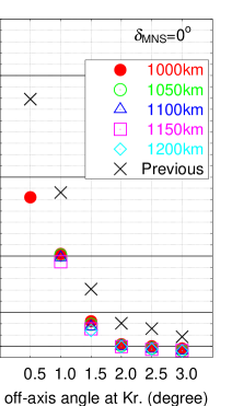
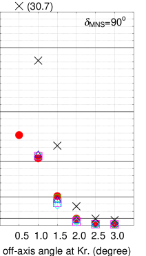
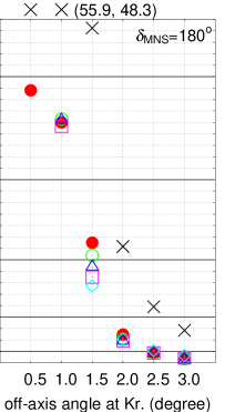
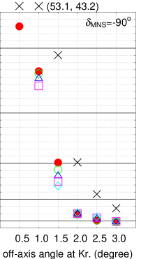
(b) inverted hierarchy (OAB:3.0@SK)

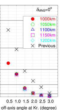
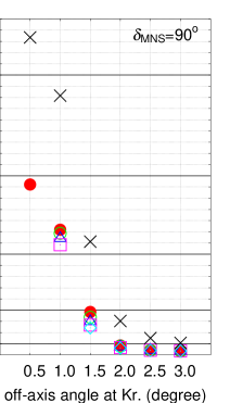
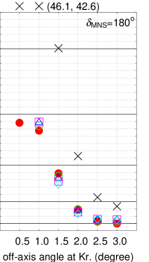
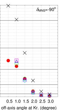
Figure 7: (a): Minimum $\Delta\chi^{2}$ of the T2KK experiment as a function of the off-axis angle and the baseline length ($L$) of a far detector from J-PARC, after $5\times 10^{21}$ POT exposure of the $3.0^{\circ}$ OAB at SK with a water $\check{\rm C}$erenkov detector of 100 kton fiducial volume in Korea. The normal hierarchy is assumed in generating the events and the inverted hierarchy is assumed in the fit. The solid-circle, open-circle, open-triangle, open-square, and open-diamond, shows $\Delta\chi^{2}_{\rm min}$ for $L=1000$ km, 1050 km, 1100 km, 1150 km, and 1200 km, respectively. We take $\sin^{2}2\theta_{\scriptscriptstyle{\rm RCT}}=0.1$ for all figures and $\delta_{\scriptscriptstyle{\rm MNS}}=0^{\circ}$, $90^{\circ}$, $180^{\circ}$, and $-90^{\circ}$, from the left to the right plots. All the other input parameters are listed in eqs. (43)-(45). The cross symbols show the highest $\Delta\chi^{2}_{\rm min}$ value of the previous study in ref. [24]. (b): The same as (a), but the inverted hierarchy is assumed in generating the events and the normal hierarchy is assumed in the fit.

We show in Fig. 7 the minimum $\Delta\chi^{2}$ expected for the T2KK experiment after $5\times 10^{21}$ POT exposure as a function of the off-axis angle and the baseline length ($L$) of the far detector in Korea, when the off-axis angle is $3.0^{\circ}$ at SK. Figure 7(a) shows the results when the normal hierarchy is assumed in generating the events and the inverted hierarchy is assumed in the fit. The opposite case, the results when the events are generated for the inverted hierarchy and the normal hierarchy is assumed in the fit are shown in Fig. 7(b). The solid-circle, open-circle, open-triangle, open-square, and open-diamond, give the minimum $\Delta\chi^{2}$ for the baseline length $L=1000$ km, 1050 km, 1100 km, 1150 km, and 1200 km, respectively. The results depend strongly on the input values of $\sin^{2}2\theta_{\scriptscriptstyle{\rm RCT}}$ and $\delta_{\scriptscriptstyle{\rm MNS}}$: $\sin^{2}2\theta_{\scriptscriptstyle{\rm RCT}}=0.1$ is assumed for all the plots and $\delta_{\scriptscriptstyle{\rm MNS}}$ is $0^{\circ}$, $90^{\circ}$, $180^{\circ}$, and $-90^{\circ}$, from the left to the right plots. All the other input parameters are listed in eqs. (43)-(45). In each plot, we show by the cross symbols the highest $\Delta\chi^{2}_{\rm min}$ values of the previous study in ref. [24]. When they are higher then 30, the cross symbols are given on top of the frame and their values are shown in parentheses.

All the plots in Fig. 7 confirm the trend observed in the previous studies in ref. [23, 24] that the sensitivity to the neutrino mass hierarchy is highest when the off-axis angle at a far detector is smallest and that there is little dependence on the baseline length between $1000$ km and $1200$ km. This is essentially because the first oscillation maximum in the $\nu_{\mu}$-to-$\nu_{e}$ transition probability occurs at around $E_{\nu}=2$ GeV in Korea, which can be observed via the wide-band beam of small off-axis angle but not with the narrow-band beam with $~{}{\hbox to0.0pt{\lower 3.5pt\hbox{$\mathchar 0\relax\sim$}\hss}\raise 1.0pt\hbox{$>$}}\,2.0^{\circ}$ off-axis angle [23, 24]. It is re-assuring that the mass hierarchy pattern can still be determined at $3\sigma$ level just by adding a $100$ kton level water $\check{\rm C}$erenkov detector at a right place (off-axis angle $~{}{\hbox to0.0pt{\lower 3.5pt\hbox{$\mathchar 0\relax\sim$}\hss}\raise 1.0pt\hbox{$<$}}\,1^{\circ}$) in Korea during the T2K experimental period ($5\times 10^{21}$POT), even after the realistic estimation for the reconstructed energy resolution and the background from single $\pi^{0}$ production via neutral current are taken into account.

Unfortunately, the reduction of the $\Delta\chi^{2}_{\rm min}$ values from the previous results are most significant at lower off-axis angles $(~{}{\hbox to0.0pt{\lower 3.5pt\hbox{$\mathchar 0\relax\sim$}\hss}\raise 1.0pt\hbox{$<$}}\,1^{\circ})$ where the mass hierarchy discrimination power of the T2KK experiment is highest. This is because the high-energy tail of the wide-band beam that gives the high sensitivity to the mass hierarchy also gives rise to the higher rate of the single $\pi^{0}$ events via the neutral currents, as shown in Fig. 4(a). This results in the larger $\pi^{0}$ background to the $\nu_{\mu}$-to-$\nu_{e}$ oscillation signal at a far detector; see Figs. 6(b) and (d). At the most favorable location of $0.5^{\circ}$ OAB at $L=1000$ km, the reduction in $\Delta\chi^{2}_{\rm min}$ is as large as $40\%$ to $60\%$, depending on $\delta_{\scriptscriptstyle{\rm MNS}}$ and the hierarchy. We also note that the $\delta_{\scriptscriptstyle{\rm MNS}}$-dependence of the sensitivity to the mass hierarchy is somewhat smaller than that of the previous analysis: For instance, the reduction of $\Delta\chi^{2}_{\rm min}$ value is largest for $\delta_{\scriptscriptstyle{\rm MNS}}=180^{\circ}$ in Fig. 7, where the highest $\Delta\chi^{2}_{\rm min}$ value was reported in ref. [24]. This is because the contribution proportional to $\cos\delta_{\scriptscriptstyle{\rm MNS}}$ in the “phase-shift” term $B^{e}$ in eq. (24b) is made less effective in discriminating the hierarchy by the smearing in $E_{\rm rec}$ due to the nucleon Fermi motion and the finite detector resolutions, which have not been taken into account in ref. [23, 24].

	$\delta_{\scriptscriptstyle{\rm MNS}}^{\rm input}$
parameters	$0^{\circ}$	$90^{\circ}$	$180^{\circ}$	$-90^{\circ}$
$\sin^{2}2\theta_{\scriptscriptstyle{\rm RCT}}$	0.74	0.18	0.90	1.8
$\sin^{2}2\theta_{\scriptscriptstyle{\rm SOL}}$	0.024	-0.010	0.052	0.12
$\delta m^{2}_{12}$	0.14	0.067	0.35	0.48
$f_{\rho}^{\rm SK}$	0.090	0.10	0.083	0.061
$f_{\rho}^{\rm Kr}$	-0.67	-0.55	-0.86	-1.0
$f_{\nu_{\mu}}^{\rm SK}$	-0.31	-0.28	-0.25	-0.21
$f_{\bar{\nu}_{\mu}}^{\rm SK}$	0.032	0.036	0.036	0.027
$f_{\nu_{e}}^{\rm SK}$	-0.050	-0.067	-0.077	-0.056
$f_{\bar{\nu}_{e}}^{\rm SK}$	-0.0013	-0.0026	0.0044	-0.0038
$f_{\nu_{\mu}}^{\rm Kr}$	0.14	0.086	0.13	0.18
$f_{\bar{\nu}_{\mu}}^{\rm Kr}$	0.0034	0.015	0.011	0.0063
$f_{\nu_{e}}^{\rm Kr}$	0.068	0.068	0.078	0.084
$f_{\bar{\nu}_{e}}^{\rm Kr}$	0.0052	0.0042	0.0042	0.0038
$f_{\nu}^{\rm CCQE}$	-0.16	-0.20	-0.14	-0.029
$f_{\bar{\nu}}^{\rm CCQE}$	0.032	0.041	0.039	0.031
$f_{\nu}^{\rm Res}$	0.13	0.085	0.099	0.11
$f_{\bar{\nu}}^{\rm Res}$	0.043	0.075	0.055	0.031
$f_{\pi^{0}}$	-0.13	-0.10	0.047	0.12
$f_{V}^{\rm SK}$	-0.33	0.32	0.30	0.24
$f_{V}^{\rm Kr}$	0.22	0.17	0.22	0.27
$\varepsilon_{e}$	0.48	0.11	0.61	1.2
$\varepsilon_{\mu}$	-0.12	-0.066	-0.14	-0.23
$P_{e/\mu}$	0.48	0.71	1.3	1.2
$\chi^{2}_{\rm para}$+$\chi^{2}_{\rm sys}$	1.8	1.2	4.0	7.6
($\chi^{2}_{\rm para}$+$\chi^{2}_{\rm sys}$)/$\Delta\chi^{2}_{\rm min}$	0.13	0.091	0.17	0.27

Table 2: The pull factors of the parameters that characterize systematic errors at $\Delta\chi^{2}_{\rm min}$ for $3.0^{\circ}$ OAB at SK and $0.5^{\circ}$ OAB at $L=1000$ km, when the normal hierarchy is assumed in generating the events and the inverted hierarchy is assumed in the fit. The model parameters are taken as in eqs. (43)-(45) for $\sin^{2}2\theta_{\scriptscriptstyle{\rm RCT}}=0.1$ and $\delta_{\scriptscriptstyle{\rm MNS}}=0^{\circ}$, $90^{\circ}$, $180^{\circ}$, and $-90^{\circ}$. The pull factors whose magnitudes are larger than unity are shown by bold face letters. The bottom lines give the squared sum of all the pull factors and its fraction in the total $\Delta\chi^{2}_{\rm min}$.

In Table 2, we list the pull factors of all the parameters for systematic errors at $\Delta\chi^{2}_{\rm min}$, for $3.0^{\circ}$ OAB at SK and $0.5^{\circ}$ OAB at $L=1000$ km, for the normal hierarchy and for all the four $\delta_{\scriptscriptstyle{\rm MNS}}$ values in Fig. 7(a). It is clearly seen that the pull factors for $\sin^{2}2\theta_{\scriptscriptstyle{\rm RCT}}$, $f_{\rho}^{\rm Kr}$, $\varepsilon_{e}$, and $P_{e/\mu}$ are most significant. The $\sin^{2}2\theta_{\scriptscriptstyle{\rm RCT}}^{\rm fit}$ is shifted upwards in order to compensate for the small event numbers expected for the inverted hierarchy. The matter density between J-PARC and Korea is reduced to make the matter effect in the wrong sign small. On the other hand, $\rho_{\rm SK}$ is slightly shifted in the positive direction, because it is the difference in the matter effects along the two baselines that is sensitive to the mass hierarchy. The positive pull factors of $\varepsilon_{e}$ and $P_{e/\mu}$ also increase the number of $e$-like events at a far detector in Korea. Reduction of these errors, in particular that of $\sin^{2}2\theta_{\scriptscriptstyle{\rm RCT}}$ by the next-generation reactor experiments, should hence improve the sensitivity of the T2KK experiment on the neutrino mass hierarchy. On the other hand, the fraction of the systematic errors in the total $\Delta\chi^{2}_{\rm min}$ is not large for a 100 kton detector with $5\times 10^{21}$POT, as shown in the bottom line of Table 2. Therefore, a larger detector and/or higher beam power will improve the sensitivity of the experiment.

		$\delta_{\scriptscriptstyle{\rm MNS}}^{\rm input}$
	analysis condition	$0^{\circ}$	$90^{\circ}$	$180^{\circ}$	$-90^{\circ}$
(0)	previous results [24]	22.9	30.7	55.9	53.1
(1)	$\rho_{\rm SK}/\rho_{\rm Kr}=2.6/3.0\times(1\pm 0.06)$ g/cm3, $\varepsilon_{\mu}=(100^{+0}_{-1})\%$	22.8	30.3	54.0	50.5
(2)	$\varepsilon_{e}=(90\pm 5)\%$	20.4	26.8	47.4	42.7
(3)	$E_{\rm rec}$ for event energy with detector resolution	18.3	23.3	39.8	37.1
(4)	$P_{e/\mu}=(1\pm 1)\%$	17.4	19.8	31.7	31.5
(5)	$\pi^{0}$ background	11.1	10.3	20.7	23.2
(6)	non-CCQE “resonance” events	14.2	12.7	23.8	28.0

Table 3: Changes in $\Delta\chi^{2}_{\rm min}$ with various assumptions on the systematic effects of the T2KK experiment, for the combination of $3.0^{\circ}$ OAB at SK and $0.5^{\circ}$ OAB at $L=1000$ km, when the normal hierarchy is assumed in generating the events and the inverted hierarchy in the fit. We take $\sin^{2}2\theta_{\scriptscriptstyle{\rm RCT}}=0.1$ and $\delta_{\scriptscriptstyle{\rm MNS}}=0^{\circ}$, $90^{\circ}$, $180^{\circ}$, and $-90^{\circ}$ as inputs and all the others are as in eqs. (43)-(45). The top (0) row gives the previous results of ref. [24], and each row gives the results after changing the conditions one by one. The bottom (6) row gives our results shown in Fig. 7(a)

(a) normal hierarchy (OAB:2.5@SK)

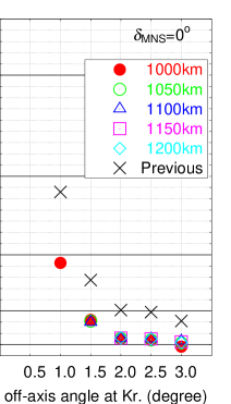
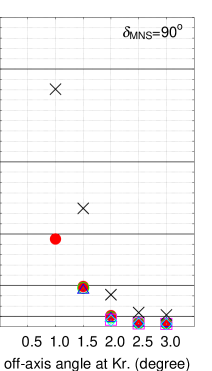
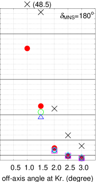
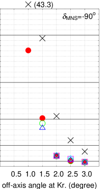
(b) inverted hierarchy (OAB:2.5@SK)

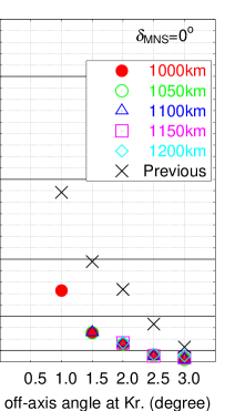
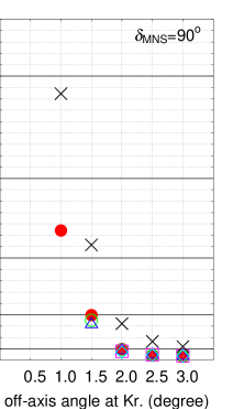
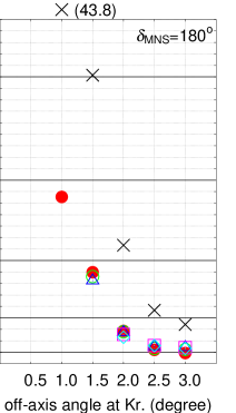
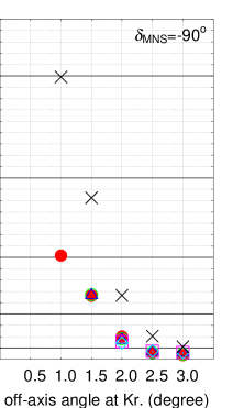
Figure 8: The same as Figure 7, but with $2.5^{\circ}$ OAB at SK.

In Table 3, we show how $\Delta\chi^{2}_{\rm min}$ changes from the values in ref. [24] by adding successively the effects introduced in this analysis, for the combination of $3.0^{\circ}$ OAB at SK and $0.5^{\circ}$ OAB at $L=1000$ km, when the normal hierarchy is assumed in generating the events and the inverted hierarchy is assumed in the fit. The first row (0) gives the results of the previous study in ref. [24]. In the row (1), we change the average matter density along the T2K baseline from 2.8 to 2.6 g/cm³ and the error of $\rho_{\rm SK}$ and $\rho_{\rm Kr}$ are doubled from $3\%$ to $6\%$, and we also introduced a $1\%$ error in the $\mu$ detection efficiency. The $\Delta\chi^{2}$ values are slightly reduced for $\delta_{\scriptscriptstyle{\rm MNS}}=180^{\circ}$ and $-90^{\circ}$ cases, mainly because of the increase in the matter density errors. In the row (2), we further introduce the detection efficiency for the $e$-like events, $\varepsilon_{e}=(90\pm 5)\%$, and the $\Delta\chi^{2}_{\rm min}$ for all $\delta_{\scriptscriptstyle{\rm MNS}}$ decrease by about $10\%$ reflecting the $10\%$ decrease of the signal events. In the row (3), we introduce smearing in $E_{\rm rec}$ due to the nuclear Fermion motion and realistic energy resolution of detectors. Because the matter effects in the phase-shift term $B^{e}$ is diluted by the smearing, the decrease in $\Delta\chi^{2}_{\rm min}$ is largest $\delta=180^{\circ}$; see the term proportional to $\cos\delta_{\scriptscriptstyle{\rm MNS}}$ in eq. (24b). In the row (4), we take into account the particle misidentification probability $P_{e/\mu}=(1\pm 1)\%$. Since this change makes the fake $e$-like events around the dip of the $\nu_{\mu}\to\nu_{e}$ transition probability, the reduction in $\Delta\chi^{2}_{\rm min}$ is significant even for $1\%$ misidentification probability, if its error is as large as $100\%$. In the row (5), the single $\pi^{0}$ events reduce the physics potential of the T2KK experiment significantly, because the $\nu_{\mu}\to\nu_{e}$ signal at small $E_{\rm rec}$ is dominated by the $\pi^{0}$ background at a far detector in Korea, as shown in Fig. 6. In the bottom row (6), we add the non-CCQE “resonance” events in the analysis. These events make $\Delta\chi^{2}_{\rm min}$ large, because their magnitudes are also proportional to the $\nu_{\mu}\to\nu_{e}$ transition probability.

In Fig. 8, we show the minimum $\Delta\chi^{2}$, the mass hierarchy discrimination power of the T2KK experiment, when the beam center is $2.5^{\circ}$ below the SK. All the other contents of Fig. 8 are the same as those of Fig. 7. Because of the geological constraint, the $2.5^{\circ}$ OAB at SK cannot provide $0.5^{\circ}$ OAB in Korean peninsula [23, 24]. When the off-axis angle is $2.5^{\circ}$ at SK, the optimum OAB for a far detector in Korea is $1.0^{\circ}$ at $L=1000$ km. The value of $\Delta\chi^{2}_{\rm min}$ is not significantly different between the $3.0^{\circ}$ OAB at SK and the $2.5^{\circ}$ OAB at SK, when the off-axis angle in Korea is fixed as $1.0^{\circ}$. It confirms our understanding that the energy profile or the hardness of the neutrino beam observed at a far detector is essential for the mass hierarchy discrimination.

5.2 Uncertainty of the $\pi^{0}$ background

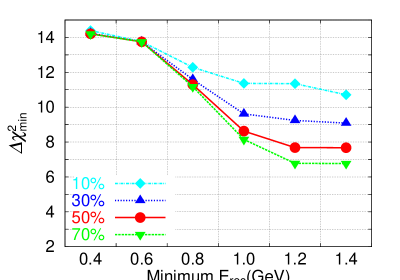
Figure 9: Minimum $\Delta\chi^{2}$ of the T2KK experiment as a function of the minimum $E_{\rm rec}$, when only those $e$-like events with larger $E_{\rm rec}$ values are retained in the analysis at a far detector. The events are calculated for the $3.0^{\circ}$ OAB at SK and a 100 kton water $\check{\rm C}$erenkov detector at $0.5^{\circ}$ OAB and $L=1000$ km with $5\times 10^{21}$ POT exposure, for $\sin^{2}2\theta_{\scriptscriptstyle{\rm RCT}}=0.1$ and $\delta_{\scriptscriptstyle{\rm MNS}}=0^{\circ}$ and the parameters of eqs. (43)-(45), for the normal hierarchy, while the inverted hierarchy is assumed in the fit. The dashed-dotted line with diamonds, the dotted line with up-triangles, the solid line with circles, and the dashed line with down-triangles give $\Delta\chi^{2}_{\rm min}$ when the uncertainty in the $\pi^{0}$ background rate $\Delta f_{\pi^{0}}$ is $10\%$, $30\%$, $50\%$, and $70\%$, respectively.

In this subsection, we examine the impacts of the $\pi^{0}$ background in more detail. In our analysis, we adopt the following uncertainties for the relevant cross sections

$$f_{\beta}^{\rm CCQE}=1\pm 0.03\,,\hskip 21.52771ptf_{\beta}^{\rm Res}=1\pm 0.2\,,\hskip 21.52771ptf_{\pi^{0}}=1\pm 0.5\,,$$ (52)

where $\beta=\nu$ and $\bar{\nu}$; see eq. (50). The $3\%$ error in the CCQE cross sections should be achieved in the near future, whereas there is a possibility that the non-CCQE “resonance” cross sections and the neutral current single $\pi^{0}$ production cross section can be measured more accurately than $20\%$ and $50\%$, respectively, assumed in this analysis. We therefore repeat the fit by varying $\Delta f_{\beta}^{\rm Res}$ between $10\%$ and $30\%$, and $\Delta f_{\pi^{0}}$ between $10\%$ and $70\%$. We find little impacts of those variations on the magnitude of $\Delta\chi^{2}_{\rm min}$, which conform with the small pull factors for these parameters in Table 2. It turns out that the uncertainty in the non-CCQE cross section does not affect the mass hierarchy sensitivity of the T2KK experiment because it tends to cancel in the ratio of the $\mu$-like and $e$-like events.

In case of the $\pi^{0}$ background to the $e$-like events, however, the smallness of the impacts of varying $\Delta f_{\pi^{0}}$ between $10\%$ and $70\%$ is striking, and we examine the cause carefully. In Fig. 9, we show $\Delta\chi^{2}_{\rm min}$ of the T2KK experiment as a function of the lowest $E_{\rm rec}$ above which the $e$-like events are counted at the far detector in Korea. All the other conditions and the input parameters are the same as those of Fig. 7(a) and Table 3, for $\delta_{\scriptscriptstyle{\rm MNS}}=0^{\circ}$. The dash-dotted line with diamonds, the dotted line with upper triangles, the solid line with circles, and the dashed line with lower triangles are obtained with the $\pi^{0}$ background normalization error of $\Delta f_{\pi^{0}}=10\%$, $30\%$, $50\%$, and $70\%$, respectively.

It is clearly seen that there is little dependence on the error $\Delta f_{\pi^{0}}$ when we use all the data with $E_{\rm rec}\geq 0.4$ GeV as has been assumed in our analysis. As the $E_{\rm rec}$ threshold is increased, however, the reduction in $\Delta\chi^{2}_{\rm min}$ becomes significant as $\Delta f_{\pi^{0}}$ increases. This is because the normalization of the $\pi^{0}$ background can be determined by the $e$-like event rate at low $E_{\rm rec}$ where the $\pi^{0}$ background dominates the oscillation signal; see Fig. 6(b) and (d). This suggests strongly that we should understand not only the overall normalization of the $\pi^{0}$ background but also the energy and angular distribution of singly produced $\pi^{0}$’s in the neutral current events as well as the momentum dependence of the error of the $\pi^{0}$-to-$e$ misidentification probability $P_{e/\pi^{0}}$, whose parameterization is given in Fig. 4(b). Detailed studies of the normalization and the shape of the $\pi^{0}$ background should be the most important task before the physics case of the T2KK experiment can be established.

5.3 Dependence of the OAB at SK

In Figs. 7 and 8, we find that the best location of the far detector to determine the neutrino mass hierarchy is at $L=1000$ km away from the J-PARC, where $0.5^{\circ}$ OAB can be observed for the $3.0^{\circ}$ OAB at SK (Fig. 7), or $1.0^{\circ}$ OAB for the $2.5^{\circ}$ OAB at SK (Fig. 8). In this subsection, we compare carefully the two combinations since they can be interchanged, or the $(1.0-\theta)^{\circ}$ OAB can be observed for the $(2.5+\theta)^{\circ}$ OAB at SK, simply by adjusting the beam direction at J-PARC (up to $|\theta|~{}{\hbox to0.0pt{\lower 3.5pt\hbox{$\mathchar 0\relax\sim$}\hss}\raise 1.0pt\hbox{$<$}}\,0.5^{\circ}$) for a fixed far detector location along the baseline at $L\simeq 1000$ km.

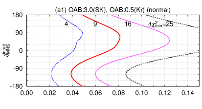
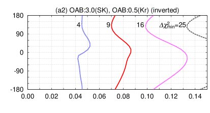
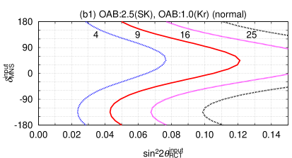
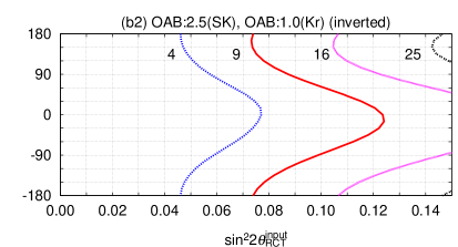
Figure 10: The $\Delta\chi^{2}_{\rm min}$ contour plot for the capability of the T2KK experiment to determine the neutrino mass hierarchy on the $\sin^{2}2\theta_{\scriptscriptstyle{\rm RCT}}^{\rm input}$ and $\delta_{\scriptscriptstyle{\rm MNS}}^{\rm input}$ plain. (a1) and (b1) are for the normal hierarchy, while (a2) and (b2) are for the inverted hierarchy. The OAB combination for (a1) and (a2) is $3.0^{\circ}$ OAB at SK and $0.5^{\circ}$ OAB at $L=1000$ km, $2.5^{\circ}$ OAB at SK and $1.0^{\circ}$ OAB at $L=1000$ km is for (b1) and (b2). All the input parameters other than $\sin^{2}2\theta_{\scriptscriptstyle{\rm RCT}}^{\rm input}$ and $\delta_{\scriptscriptstyle{\rm MNS}}^{\rm input}$ are the same as those in Figs. 7 and 8.

In Fig. 10, we show the contours for $\Delta\chi^{2}_{\rm min}=4$, $9$, $16$, $25$ in the plane of $\sin^{2}2\theta_{\scriptscriptstyle{\rm RCT}}^{\rm input}$ and $\delta_{\scriptscriptstyle{\rm MNS}}^{\rm input}$. The wrong hierarchy can be excluded with the $n$-$\sigma$ confidence level, if the true values of $\sin^{2}2\theta_{\scriptscriptstyle{\rm RCT}}$ and $\delta_{\scriptscriptstyle{\rm MNS}}$ lie in the right-hand side of the $\Delta\chi^{2}_{\rm min}=n^{2}$ contour. The upper figures (a1) and (a2) are for $3.0^{\circ}$ OAB at SK with $0.5^{\circ}$ OAB at $L=1000$ km, and the lower figures (b1) and (b2) are for the $2.5^{\circ}$ OAB at SK with $1.0^{\circ}$ OAB also at $L=1000$ km.

It is clearly seen from the figures that the mass hierarchy can be determined better by the combination of $3.0^{\circ}$ OAB at SK and $0.5^{\circ}$ OAB at $L=1000$ km than the combination of $2.5^{\circ}$ and $1.0^{\circ}$ for all the input values of $\sin^{2}2\theta_{\scriptscriptstyle{\rm RCT}}$ and $\delta_{\scriptscriptstyle{\rm MNS}}$ and for both hierarchy patterns. For instance, by comparing the figures (a1) and (b1) we find that the normal hierarchy can be established at $3\sigma$ level, $\Delta\chi^{2}_{\rm min}>9$, when $\sin^{2}2\theta_{\scriptscriptstyle{\rm RCT}}~{}{\hbox to0.0pt{\lower 3.5pt\hbox{$\mathchar 0\relax\sim$}\hss}\raise 1.0pt\hbox{$>$}}\,0.08$ $(0.12)$ for the combination of $3.0^{\circ}$ and $0.5^{\circ}$ ($2.5^{\circ}$ and $1.0^{\circ}$). Likewise, from the figures (a2) and (b2), the inverted hierarchy can be established when $\sin^{2}2\theta_{\scriptscriptstyle{\rm RCT}}~{}{\hbox to0.0pt{\lower 3.5pt\hbox{$\mathchar 0\relax\sim$}\hss}\raise 1.0pt\hbox{$>$}}\,0.09$ $(0.12)$ for the combination of $3.0^{\circ}$ and $0.5^{\circ}$ ($2.5^{\circ}$ and $1.0^{\circ}$). The difference is significant when $|\delta_{\scriptscriptstyle{\rm MNS}}|~{}{\hbox to0.0pt{\lower 3.5pt\hbox{$\mathchar 0\relax\sim$}\hss}\raise 1.0pt\hbox{$<$}}\,90^{\circ}$ where it is difficult to determine the mass hierarchy. On the other hand, we find little dependence on the off-axis angle between $3.0^{\circ}$ and $2.5^{\circ}$ at SK when $\delta_{\scriptscriptstyle{\rm MNS}}\simeq 180^{\circ}$, where the mass hierarchy can be determined with relative ease.

The reason for the strong dependence on the off-axis angle when $|\delta_{\scriptscriptstyle{\rm MNS}}|~{}{\hbox to0.0pt{\lower 3.5pt\hbox{$\mathchar 0\relax\sim$}\hss}\raise 1.0pt\hbox{$<$}}\,90^{\circ}$ can be explained by the hardness of the $0.5^{\circ}$ OAB that provides sufficient flux at the $\nu_{\mu}\to\nu_{e}$ oscillation maximum around $E_{\nu}\sim 2.0$ GeV. It is essentially the mass hierarchy dependence of the amplitude shift term, $A^{e}$, in eqs. (22) and (24a), which contribute to the determination, and the hardness of the $0.5^{\circ}$ OAB helps enhancing the signal. When $\delta_{\scriptscriptstyle{\rm MNS}}\simeq 180^{\circ}$, in addition to the amplitude shift term, the phase-shift term $B^{e}$, in eq. (22), becomes significant because the leading term and the sub-leading term in eq. (24b) adds up to make $|B^{e}|$ large at $\cos\delta_{\scriptscriptstyle{\rm MNS}}\simeq-1$. The mass hierarchy dependence due to the phase shift term $B^{e}$ turns out to give significant difference in the $\nu_{\mu}\to\nu_{e}$ transition probability at lower $E_{\nu}$ [23, 24], and the downward shift of the flux maximum $E_{\nu}$ in the $1.0^{\circ}$ OAB can be compensated for.

In the absence of a concrete evidence that the nature chooses $\cos\delta_{\scriptscriptstyle{\rm MNS}}\simeq 180^{\circ}$, it is clear that the effort to make the off-axis angle at the far detector as small as possible should be valuable. The sensitivity difference between $0.5^{\circ}$ OAB and $1.0^{\circ}$ OAB in Fig. 10 corresponds to about a factor of two difference in the product of the fiducial volume of the far detector and the POT, the beam power times the running period.

5.4 Impacts on the $|\delta m^{2}_{13}|$ measurement

In this subsection, we comment on the implication of the mass hierarchy uncertainty in the measurement of the absolute value of the larger mass-squared difference.

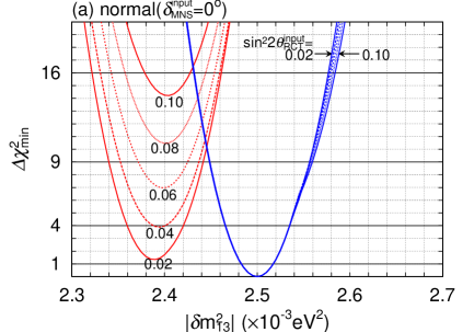
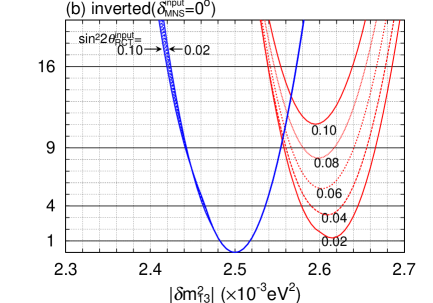
Figure 11: $\Delta\chi^{2}_{\rm min}$ of the T2KK experiment as a function of $|\delta m^{2}_{13}|$ for $3.0^{\circ}$ OAB at SK and $0.5^{\circ}$ OAB at $L=1000$ km. (a): The normal hierarchy case at $\delta_{\scriptscriptstyle{\rm MNS}}^{\rm input}=0^{\circ}$. The solid line, long-dashed, short-dashed, dotted, and the solid line again, show the results for $\sin^{2}2\theta_{\scriptscriptstyle{\rm RCT}}^{\rm input}=0.02$, $0.04$, $0.06$, $0.08$, and $0.1$, respectively. All the other input parameters are those in eqs. (43)-(45). The blue lines, which are almost degenerate, are obtained when the right hierarchy is chosen in the fit, whereas the red lines are obtained with the wrong hierarchy. (b): The inverted hierarchy case.

In Fig. 11, we show the minimum $\Delta\chi^{2}$ of the T2KK experiment as a function of $|\delta m^{2}_{13}|$ with the optimum OAB combination of $3.0^{\circ}$ at SK and $0.5^{\circ}$ at $L=1000$ km. Fig. 11(a) is for the normal hierarchy and Fig. 11(b) is for the inverted hierarchy. The five curves are for $\sin^{2}2\theta_{\scriptscriptstyle{\rm RCT}}^{\rm input}=0.02$, $0.04$, $0.06$, $0.08$, and $0.1$, which are denoted by the solid, long-dashed, short-dashed, dotted, and the solid line again, respectively. The CP phase is fixed at $\delta_{\scriptscriptstyle{\rm MNS}}=0^{\circ}$ and all the other parameters are those of eqs. (43)-(45). In both cases there is a set of five curves with $\Delta\chi^{2}_{\rm min}=0^{\circ}$ at $|\delta m^{2}_{13}|=2.5\times 10^{-3}$ eV², the input value. All the five curves are almost degenerate in the set, which exhibits the insensitivity of the $\nu_{\mu}\to\nu_{\mu}$ survival probability on $\sin^{2}2\theta_{\scriptscriptstyle{\rm RCT}}$; see eqs. (21a) and (23). On the other hand, there is another set of five curves with $\Delta\chi^{2}_{\rm min}$ at $0.1\times 10^{-3}$ eV² smaller (larger) than the input value when the mass hierarchy is normal (inverted). These curves with $\sin^{2}2\theta_{\scriptscriptstyle{\rm RCT}}$ dependent $\Delta\chi^{2}_{\rm min}$ are obtained when the opposite hierarchy is assumed in the fit.

The larger mass-squared difference is determined from the T2KK experiment correctly as

$$\left|\delta m^{2}_{13}\right|=\left(2.5\pm 0.02\right)\times 10^{-3}\mbox{{eV${}^{2}$}}\,,$$ (53)

if we know the mass hierarchy pattern. However, if we do not know the mass hierarchy pattern, the other solution

$$\left|\delta m^{2}_{13}\right| \simeq (2.4\pm 0.02)\times 10^{-3}\mbox{{eV${}^{2}$~{}~{}~{}~{}(for the normal hierarchy)}}\,,$$ (54)

$$\simeq (2.6\pm 0.02)\times 10^{-3}\mbox{{eV${}^{2}$~{}~{}~{}~{}(for the inverted hierarchy)}}\,,$$

appears for every $\sin^{2}2\theta_{\scriptscriptstyle{\rm RCT}}^{\rm input}$. The wrong solution (54) are about $3.5\sigma$ away from the correct solution (53). The difference of $\mp 0.1\times 10^{-3}$ eV² in the mean value can be explained by the phase shift term $B^{\mu}$ in the $\nu_{\mu}\to\nu_{\mu}$ survival probability; see eqs. (21a) and (23b). From the peak location at

$$\frac{\Delta_{13}}{2}+B^{\mu}=\displaystyle\frac{\pi}{2}\,,$$ (55)

the location of the solution with the wrong hierarchy can be estimated as

$$\left|\left(\delta m^{2}_{13}\right)^{\rm fit}\right|-\left|\left(\delta m^{2}_{13}\right)^{\rm input}\right|$$ (56)

$$\simeq -\displaystyle\frac{\left(\delta m^{2}_{13}\right)^{\rm input}}{\left|\left(\delta m^{2}_{13}\right)^{\rm input}\right|}\left(0.11-0.023\left(\displaystyle\frac{\sin^{2}2\theta_{\scriptscriptstyle{\rm RCT}}^{\rm input}}{0.10}\right)^{1/2}\cos\delta_{\scriptscriptstyle{\rm MNS}}^{\rm input}\right)\times 10^{-3}\mbox{{eV${}^{2}$}}\,.$$

The magnitude of the difference is almost $0.09\times 10^{-3}$ eV² for $\sin^{2}2\theta_{\scriptscriptstyle{\rm RCT}}^{\rm input}=0.1$ at $\cos\delta_{\scriptscriptstyle{\rm MNS}}^{\rm input}=1$, and it grows to $0.11\times 10^{-3}$ eV² as $\sin^{2}2\theta_{\scriptscriptstyle{\rm RCT}}$ decreases, as can be observed from the figures. This result suggests that the absolute value of the larger mass-squared difference cannot be determined uniquely, if the mass hierarchy pattern is not known. Because the T2KK experiment can determine the mass hierarchy from the $\nu_{\mu}\to\nu_{e}$ transition rates for sufficiently large $\sin^{2}2\theta_{\scriptscriptstyle{\rm RCT}}^{\rm input}$, the fake $|\delta m^{2}_{13}|$ can be excluded for larger $\sin^{2}2\theta_{\scriptscriptstyle{\rm RCT}}^{\rm input}$ as shown by the $\Delta\chi^{2}_{\rm min}$ values of the wrong solutions in Figs. 11(a) and (b), which grow with increasing $\sin^{2}2\theta_{\scriptscriptstyle{\rm RCT}}^{\rm input}$. If we do not make use of the $\nu_{\mu}\to\nu_{e}$ transition signal in the fit, all the solutions with the wrong mass hierarchy has $\Delta\chi^{2}_{\rm min}\simeq 0$, indistinguishable from the correct solution.

Let us note in passing that the T2K experiment suffers from the same uncertainty in the measurement of $|\delta m^{2}_{13}|$. If we drop all the data from the far detector in the above analysis with $\delta m^{2}_{13}=\pm 2.5\times 10^{-3}$ eV², we find the fake solution with

$$\left|\delta m^{2}_{13}\right| \simeq (2.4\pm 0.04)\times 10^{-3}\mbox{{eV${}^{2}$~{}~{}~{}~{}(for the normal hierarchy)}}\,,$$ (57)

$$\simeq (2.6\pm 0.04)\times 10^{-3}\mbox{{eV${}^{2}$~{}~{}~{}~{}(for the inverted hierarchy)}}\,,$$

instead of eq. (54). The $\Delta\chi^{2}_{\rm min}$ values for the wrong solutions are indistinguishable from zero for all the $\sin^{2}2\theta_{\scriptscriptstyle{\rm RCT}}$ input values. The difference of about $0.1\times 10^{-3}$ eV² between the correct and the wrong solutions remains the same, because the formulae (55) and (56) are valid near the oscillation maximum at all baseline length $L$ as long as the earth matter effect remains a small perturbation as in eqs. (21) and (23). Since the two solutions are about $2\sigma$ away, the experiment should present two values of $|\delta m^{2}_{13}|$ until the mass hierarchy is determined.

6 CP phase

In this section, we study the capability of the T2KK experiment for measuring the leptonic CP phase $\delta_{\scriptscriptstyle{\rm MNS}}$ with the optimum OAB combination, $3.0^{\circ}$ OAB at SK and $0.5^{\circ}$ OAB at $L=1000$ km, with $5\times 10^{21}$ POT exposure.

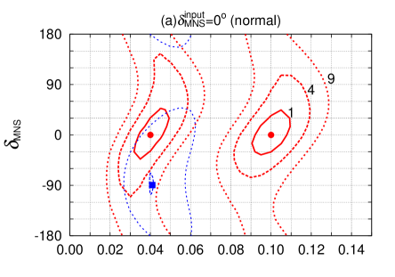
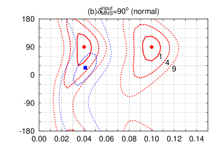
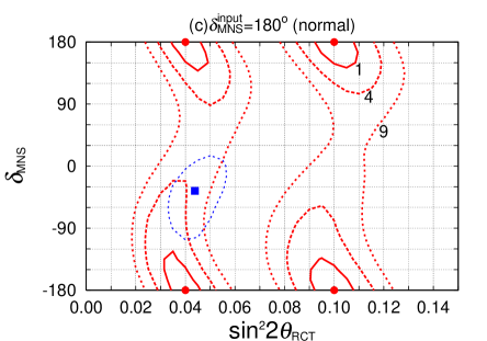
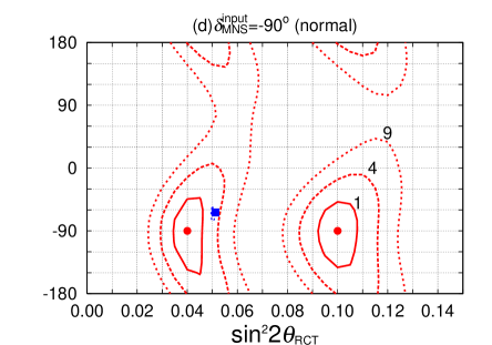
Figure 12: The $\Delta\chi^{2}$ contour plot for the T2KK experiment in the plane of $\sin^{2}2\theta_{\scriptscriptstyle{\rm RCT}}$ and $\delta_{\scriptscriptstyle{\rm MNS}}$ when the mass hierarchy is normal. Allowed regions in the plane of $\sin^{2}2\theta_{\scriptscriptstyle{\rm RCT}}$ and $\delta_{\scriptscriptstyle{\rm MNS}}$ are shown for the combination of $3.0^{\circ}$ OAB at SK and $0.5^{\circ}$ OAB at $L=1000$ km with $5\times 10^{21}$ POT. The input value of $\sin^{2}2\theta_{\scriptscriptstyle{\rm RCT}}$ is 0.10 and 0.04 for $\delta_{\scriptscriptstyle{\rm MNS}}=0^{\circ}$ (a), $\delta_{\scriptscriptstyle{\rm MNS}}=90^{\circ}$ (b), $\delta_{\scriptscriptstyle{\rm MNS}}=180^{\circ}$ (c), and $\delta_{\scriptscriptstyle{\rm MNS}}=-90^{\circ}$ (d), and the other input parameters are listed in eqs. (43)-(45). The input points are indicated as the solid blobs. The contours for $\Delta\chi^{2}=1$, $4$, and $9$ are shown by the solid, dashed, and dotted lines, respectively. The thick red contours are obtained when the right hierarchy is assumed in the fit, whereas the thin blue contours with the local minimum by the solid square show the results when the opposite mass hierarchy is assumed in the fit.

In Fig. 12, we show $\Delta\chi^{2}$ contours in the plane of $\sin^{2}2\theta_{\scriptscriptstyle{\rm RCT}}$ and $\delta_{\scriptscriptstyle{\rm MNS}}$ when the mass hierarchy is normal ($m^{2}_{3}-m^{2}_{1}>0$). The input values are $\sin^{2}2\theta_{\scriptscriptstyle{\rm RCT}}^{\rm input}=0.10$ and 0.04, and $\delta_{\scriptscriptstyle{\rm MNS}}^{\rm input}=0^{\circ}$, $90^{\circ}$, $180^{\circ}$, and $-90^{\circ}$ in Figs. (a), (b), (c), and (d), respectively. The other input parameters are those in eqs. (43)-(45). The contours for $\Delta\chi^{2}=1$, $4$, and $9$ are shown by the solid, dashed, and dotted lines, respectively. The thick red lines show the $\Delta\chi^{2}$ contours when the right hierarchy is chosen in the fit, whereas the thin blue lines show the results when the wrong hierarchy is assumed in the fit. The solid blobs in each figure denote the input points ($\Delta\chi^{2}=0$) and the solid squares are the local minima for the fit with the wrong hierarchy.

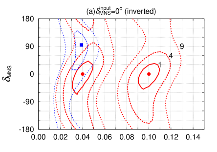
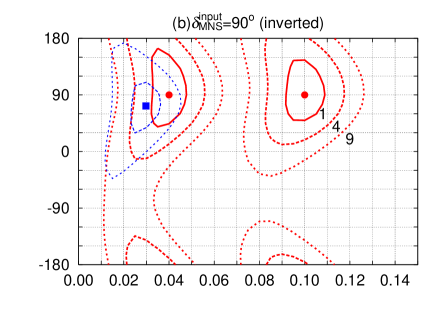
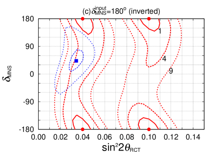
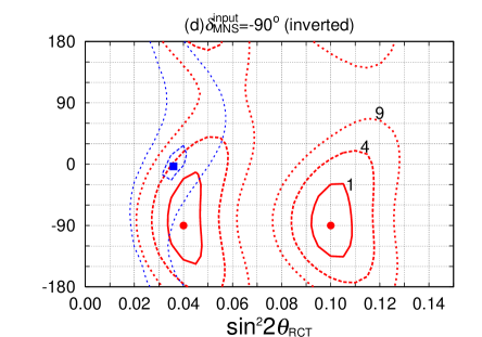
Figure 13: The same as Fig. 12, but when the mass hierarchy is inverted ($m^{2}_{3}-m^{2}_{1}<0$).

We find from the figures that $\delta_{\scriptscriptstyle{\rm MNS}}$ can be constrained to about $\pm 45^{\circ}$ at $1\sigma$ level for all the input value of $\delta_{\scriptscriptstyle{\rm MNS}}^{\rm input}$ and $\sin^{2}2\theta_{\scriptscriptstyle{\rm RCT}}$. The insensitivity of the measurement error of $\delta_{\scriptscriptstyle{\rm MNS}}$ on $\sin^{2}2\theta_{\scriptscriptstyle{\rm RCT}}$ [23, 24, 29] persists. However, at $3\sigma$ level, the contour closes only for $\delta_{\scriptscriptstyle{\rm MNS}}^{\rm input}=\pm 90^{\circ}$ at $\sin^{2}2\theta_{\scriptscriptstyle{\rm RCT}}^{\rm input}=0.1$; (b) and (d). Moreover, there appears a shadow island where the inverted hierarchy is assumed in the fit, for all the four $\delta_{\scriptscriptstyle{\rm MNS}}^{\rm input}$ cases at $\sin^{2}2\theta_{\scriptscriptstyle{\rm RCT}}^{\rm input}=0.04$. The shadow contours cover the whole $\delta_{\scriptscriptstyle{\rm MNS}}$ region when $\delta_{\scriptscriptstyle{\rm MNS}}^{\rm input}=90^{\circ}$, where the number of the $\nu_{\mu}\to\nu_{e}$ signal events is the smallest among the four $\delta_{\scriptscriptstyle{\rm MNS}}^{\rm input}$ cases.

These observations are in sharp contrast with the previous ones, shown in e.g., Fig. 8 of ref. [24], where it has been shown that the $\delta_{\scriptscriptstyle{\rm MNS}}$ can be constrained to about $\pm 30^{\circ}$ for all the four input $\delta_{\scriptscriptstyle{\rm MNS}}$ values at $\sin^{2}2\theta_{\scriptscriptstyle{\rm RCT}}^{\rm input}~{}{\hbox to0.0pt{\lower 3.5pt\hbox{$\mathchar 0\relax\sim$}\hss}\raise 1.0pt\hbox{$>$}}\,0.02$ and that the shadow islands from the wrong hierarchy solution are small and they appear only for $\delta_{\scriptscriptstyle{\rm MNS}}^{\rm input}=90^{\circ}$ at $\sin^{2}2\theta_{\scriptscriptstyle{\rm RCT}}^{\rm input}=0.04$ and for $\delta_{\scriptscriptstyle{\rm MNS}}^{\rm input}=0^{\circ}$, $90^{\circ}$, and $180^{\circ}$ at $\sin^{2}2\theta_{\scriptscriptstyle{\rm RCT}}^{\rm input}=0.02$. We find that both the reduction of the sensitivity from $\pm 30^{\circ}$ to $\pm 45^{\circ}$ and the appearance of the big shadow islands are mainly due to the $\pi^{0}$ background for the $e$-like events, while the smearing effects due to nuclear Fermi motion and the detector resolution also contribute at the sub-leading level.

In Fig. 13, we show the same contour plots as in Fig. 12, but for the inverted hierarchy case. We find that the $1\sigma$ constraints on $\delta_{\scriptscriptstyle{\rm MNS}}$ are slightly worse than those of the normal hierarchy case in Fig. 12: The $1\sigma$ error remains at about $\pm 45^{\circ}$ for $\delta_{\scriptscriptstyle{\rm MNS}}^{\rm input}=0^{\circ}$ and $180^{\circ}$, but it grows to about $\pm 60^{\circ}$ or larger for $\delta_{\scriptscriptstyle{\rm MNS}}^{\rm input}=\pm 90^{\circ}$. As in the case of the normal hierarchy, $\delta_{\scriptscriptstyle{\rm MNS}}$ can be constrained at $3\sigma$ level only for $\delta_{\scriptscriptstyle{\rm MNS}}^{\rm input}=\pm 90^{\circ}$ at $\sin^{2}2\theta_{\scriptscriptstyle{\rm RCT}}^{\rm input}=0.1$. The $2\sigma$-level shadow islands appear for all the four $\delta_{\scriptscriptstyle{\rm MNS}}^{\rm input}$ cases at $\sin^{2}2\theta_{\scriptscriptstyle{\rm RCT}}^{\rm input}=0.04$, which is consistent with the observation of Fig. 10(a2) where all $\delta_{\scriptscriptstyle{\rm MNS}}^{\rm input}$ points lie below the $\Delta\chi_{\rm min}^{2}=4$ contours. The $3\sigma$ contours of the wrong solutions, denoted by the thin blue dotted lines, cover the whole $\delta_{\scriptscriptstyle{\rm MNS}}$ region for $\delta_{\scriptscriptstyle{\rm MNS}}^{\rm input}=0^{\circ}$ and $-90^{\circ}$ at $\sin^{2}2\theta_{\scriptscriptstyle{\rm RCT}}^{\rm input}=0.04$. The significant loss of the sensitivity to $\delta_{\scriptscriptstyle{\rm MNS}}$ as compared to Fig. 9 of ref. [24] can also be explained by the $\pi^{0}$ background to the $\nu_{\mu}\to\nu_{e}$ oscillation signal.

In summary, the capability of the T2KK experiment to measure the CP phase of the lepton flavor mixing (MNS) matrix is significantly worsened by the $\pi^{0}$ background in both normal and inverted hierarchy cases. This is because the large $\pi^{0}$ background to the $\nu_{\mu}\to\nu_{e}$ oscillation signal at the far detector, as shown in Figs. 6(b) and (d), reduce significantly the sensitivity to the amplitude-shift term $A^{e}$ and the phase-shift term $B^{e}$ which have contributions proportional to $\sin\delta_{\scriptscriptstyle{\rm MNS}}$ and $\cos\delta_{\scriptscriptstyle{\rm MNS}}$, respectively [23, 24]. These terms proportional to $\Delta_{12}$ in eq. (24) can be measured by comparing the shifts at a near ($L\simeq 300$ km) and a far ($L\simeq 1000$ km) detectors [23, 24, 29] without using the $\bar{\nu}_{\mu}$ beam. Since the $\pi^{0}$ background worsens the measurements of $A^{e}$ and $B^{e}$ at the far detector, the sensitivity to $\delta_{\scriptscriptstyle{\rm MNS}}$ deteriorates significantly. The use of $\bar{\nu}_{\mu}$ beam in addition to the $\nu_{\mu}$ beam [28, 29] may be helpful in recovering the sensitivity, since at least the detector-dependent errors of the $\pi^{0}$ background events should be common for both beams.

7 Summary and conclusion

In this paper, we elaborate the previous analyses of ref. [23, 24] on the physics potential of the T2KK experiment by taking into account the smearing of reconstructed neutrino energy due to the Fermi motion of the target nucleus and the finite resolution of $e^{\pm}$ and $\mu^{\pm}$ momenta in a water $\check{\rm C}$erenkov detector. We also include the events from the non-CCQE “resonance” events that survive the CCQE event selection cut of eq. (26), and the contribution from the single $\pi^{0}$ production via the neutral current interactions, which mimic the $\nu_{e}$ appearance signal in a water $\check{\rm C}$erenkov detector.

In order to estimate the reconstructed energy ($E_{\rm rec}$) distribution efficiently, we introduce the smearing functions for the CCQE and non-CCQE “resonance” events that map the incoming neutrino energy $E_{\nu}$ onto the reconstructed energy $E_{\rm rec}$ by using the Mote Carlo event generator nuance [30]. The effect of the detector resolution for $e^{\pm}$ and $\mu^{\pm}$, see Table 1, has also been taken into account. The smearing functions for the CCQE events are given in eq. (28) with eqs. (A7)-(A6) for $\nu_{\mu}$, and eqs. (A10)-(A9) for $\nu_{e}$ . Those for non-CCQE “resonance” events are parameterized as in eq. (30) with eqs. (A15)-(A20) in the region of $0.55\leq E_{\nu}\leq 1.2$ GeV and eq. (31) with eqs. (A22)-(A27) for $1.2$ GeV$<E_{\nu}<6.0$ GeV. For estimating the background from the single $\pi^{0}$ production, we generate single $\pi^{0}$ events from the NC interactions for each off-axis beam (OAB) also by using nuance [30], and parameterize the probability that a $\pi^{0}$ is misidentified as an $e^{\pm}$-like event, $P_{e/\pi}$, in terms of the energy ratio and the opening angle of the two photons for the $\pi^{0}$ decay-in-flight; see Fig. 4(b) and eqs. (36) and (37).

We study the sensitivity of the T2KK experiment on the neutrino mass hierarchy by placing a water $\check{\rm C}$erenkov detector with 100 kton fiducial volume at various location in Korea for the $3.0^{\circ}$ and $2.5^{\circ}$ OAB at SK. The neutrino beam at an off-axis angle greater than about 0.5 (1.0) can be observed in Korea, at the baseline length $1000$ km$~{}{\hbox to0.0pt{\lower 3.5pt\hbox{$\mathchar 0\relax\sim$}\hss}\raise 1.0pt\hbox{$<$}}\,L~{}{\hbox to0.0pt{\lower 3.5pt\hbox{$\mathchar 0\relax\sim$}\hss}\raise 1.0pt\hbox{$<$}}\,1200$ km, for the $3.0^{\circ}$ OAB ($2.5^{\circ}$ OAB) at SK. We find that the highest sensitivity is achieved for the combination of $3.0^{\circ}$ OAB at SK and $0.5^{\circ}$ OAB at $L=1000$ km, confirming the results of ref. [23, 24]. With $5\times 10^{21}$ POT, which is the planned exposure of the T2K experiment, the mass hierarchy can be determined at $3\sigma$ level if $\sin^{2}2\theta_{\scriptscriptstyle{\rm RCT}}~{}{\hbox to0.0pt{\lower 3.5pt\hbox{$\mathchar 0\relax\sim$}\hss}\raise 1.0pt\hbox{$>$}}\,0.08$ ($0.09$) for the above OAB combination, when the neutrino mass hierarchy is normal (inverted). For the combination of $2.5^{\circ}$ OAB at SK and $1.0^{\circ}$ OAB at $L=1000$ km, the $3\sigma$ sensitivity is obtained for $\sin^{2}2\theta_{\scriptscriptstyle{\rm RCT}}~{}{\hbox to0.0pt{\lower 3.5pt\hbox{$\mathchar 0\relax\sim$}\hss}\raise 1.0pt\hbox{$>$}}\,0.12$ for both hierarchies; see Fig. 10 in section 5.3. These figures show significant reduction of the sensitivity as compared to the results of the previous studies, such as Fig.6 of ref. [24], which show that the neutrino mass hierarchy can be determined for $\sin^{2}2\theta_{\scriptscriptstyle{\rm RCT}}~{}{\hbox to0.0pt{\lower 3.5pt\hbox{$\mathchar 0\relax\sim$}\hss}\raise 1.0pt\hbox{$>$}}\,0.05(0.06)$ at $3\sigma$, when the hierarchy is normal (inverted), with the same combinations of the OAB’s, and with the same detector size and the POT.

We find that the main cause of the reduction in the sensitivity is the background from the single $\pi^{0}$ production; see Table 3 in section 5.1. The smearing in the reconstructed energy has a significant effect when $\delta_{\scriptscriptstyle{\rm MNS}}\simeq 180^{\circ}$, where the mass hierarchy dependent oscillation phase-shift term is large. The contribution from the non-CCQE “resonance” events help discriminating the mass hierarchy, because these events are also a part of the $\nu_{\mu}\to\nu_{e}$ oscillation signal.

We also examine the prospect of the CP phase measurement for the T2KK experiment with the above OAB combination. The sensitivity of the $\delta_{\scriptscriptstyle{\rm MNS}}$ measurement is also reduced significantly from that of the previous study in ref. [24], which found the $1\sigma$ error of about $\pm 30^{\circ}$, to about $\pm 45^{\circ}$ or even $\pm 60^{\circ}$ in some cases. The main cause of the worsening of the error is again the $\pi^{0}$ background for the $e$-like events at the far detector that makes it difficult to measure the baseline dependence of the $\nu_{\mu}\to\nu_{e}$ oscillation amplitude and the phase: $\sin\delta_{\scriptscriptstyle{\rm MNS}}$ is measured by the amplitude difference and $\cos\delta_{\scriptscriptstyle{\rm MNS}}$ is measured by the phase difference [23, 24].

The $\pi^{0}$ background reduces significantly the physics potential for the mass hierarchy determination and the CP phase measurement of the T2KK experiment. If we understand better the physics of the $\pi^{0}$ production and its decay signal inside the water $\check{\rm C}$erenkov detector, the sensitivity of the experiment on these fundamental parameters should be improved. Detailed investigation of the normalization and the shape of the $\pi^{0}$ background should be one of the most important tasks to evaluate quantitatively the physics discovery potential of the T2KK experiment.

Appendix Appendix A Smearing functions $f^{X}_{\alpha}(E_{\rm rec};E_{\nu})$

In the appendix, we show our parameterization of the smearing functions, $f^{X}_{\alpha}(E_{\rm rec};E_{\nu})$, which map the incoming neutrino energy, $E_{\nu}$, onto the reconstructed energy, $E_{\rm rec}$, for the quasi-elastic events. The superscript $X$ denotes the event type, $X=$ CCQE for the CCQE events, or $X=$ Res for the non-CCQE “resonance” events that pass the CCQE selection criteria of eq. (26), and the subscript $\alpha$ is for $\mu$ or $e$: $\alpha=\mu$ for $\nu_{\mu}$ events and $\alpha=e$ for $\nu_{e}$ events. These functions take account of the Fermi motion of the target nucleon inside the oxygen nucleus and the finite energy-momentum resolutions of a muon and an electron in a water $\check{\rm C}$erenkov detector listed in Table 1.

Appendix A.1 CCQE events

The $E_{\rm rec}$ distribution of the CCQE events, which are generated by nuance [30], can be parameterized accurately by 3 Gaussians,

$$f^{\rm CCQE}_{\alpha}(E_{\rm rec};E_{\nu})=\displaystyle\frac{1}{A^{\alpha}(E_{\nu})}\sum_{n=1}^{3}r^{\alpha}_{n}(E_{\nu})\exp\left(-\displaystyle\frac{(E_{\rm rec}-E_{\nu}+{\delta}E^{\alpha}_{n}(E_{\nu}))^{2}}{2(\sigma^{\alpha}_{n}(E_{\nu}))^{2}}\right)\,,$$ (A1)

in the region of

$$0.3\mbox{{~{}GeV}}\leq E_{\nu}\leq 6.0\mbox{{~{}GeV}}\mbox{{~{}~{}for~{}~{}}}0.4\mbox{{~{}GeV}}\leq E_{\rm rec}\leq 5.0\mbox{{~{}GeV}}\,.$$ (A2)

The index $\alpha$ takes $\mu$ for $\nu_{\mu}$ and $e$ for $\nu_{e}$ events, and each function is normalized by

$$A^{\alpha}(E_{\nu})=\sqrt{2\pi}\sum_{n=1}^{3}r^{\alpha}_{n}(E_{\nu})\sigma_{n}^{\alpha}(E_{\nu})\,.$$ (A3)

The variance $\sigma^{\alpha}_{n}$, the energy shift ${\delta}E^{\alpha}_{n}$, and the normalization factors $r^{\alpha}_{2,3}$ are functions of the incoming neutrino energy $E_{\nu}$, with $r^{\alpha}_{1}(E_{\nu})=1$. The first and the second Gaussians account mainly for the nuclear Fermi motion, and we can set $\delta E_{2}^{\mu}=\delta E_{1}^{\mu}$. The third Gaussian is necessary to account for the asymmetry in the $E_{\rm rec}-E_{\nu}$ distribution such as the Fermi block effect at the low energies, and the asymmetric momentum resolution effects at high energies.

All the coefficients are parameterized compactly by using the variables

$$x=E_{\nu}~{}\mbox{{[GeV]}}-1\,,\hskip 43.05542pt\xi=\sqrt{E_{\nu}~{}\mbox{{[GeV]}}}-1\,,$$ (A4)

which vanish at $E_{\nu}=1$ GeV. The variance $\sigma^{\mu}_{n}$(MeV) of the three Gaussians

$$\sigma^{\mu}_{1} = 39.7+68.5\xi\,,$$ (A5a)

$$\sigma^{\mu}_{2} = 82.7-50.2x+259\xi\,,$$ (A5b)

$$\sigma^{\mu}_{3} = 197+486x-606\xi+203x\xi\,,$$ (A5c)

and the energy shift terms $\delta E_{n}^{\mu}$ (MeV)

$${\delta}E^{\mu}_{1}={\delta}E^{\mu}_{2} = 35-2.5x(1-1.2x)/(1+x)\,,$$ (A6a)

$${\delta}E^{\mu}_{3} = \sigma_{3}^{\mu}\left[0.053+0.033x\left(\displaystyle\frac{1+5.27x-8.67x^{2}+1.83x^{3}}{1+3.65x+4.35x^{2}}\right)\right]\,,$$ (A6b)

are given in units of MeV. The normalization factors are $r^{\mu}_{1}=1$ and

$$r^{\mu}_{2} = 1.1-0.96x+0.44x^{2}-0.076x^{3}+0.0047x^{4}\,,$$ (A7a)

$$r^{\mu}_{3} = 0.365-1.97\xi(1-0.634\xi+0.464\xi^{2}+0.293\xi^{3}-0.342\xi^{4})/(1+1.23x)\,.~{}~{}~{}~{}~{}$$ (A7b)

The first and second variances are determined mainly by the sum of the nuclear Fermi motion and the momentum resolution of the water $\check{\rm C}$erenkov detector. In the absence of the momentum resolution error, two Gaussians, one with a constant variance of $\sim 60$ MeV and the other with a larger variance of $\sim 190$ MeV at $E_{\nu}\sim 1$ GeV which decreases slowly with energy, can account for the bulk of the Fermi motion effects on the $E_{\rm rec}-E_{\nu}$ distribution; see Fig. 1. It is the smearing effect due to the energy resolution which increases the first two variances as $\sqrt{E_{\nu}}$ at high energies. The value of $\delta E_{1,2}^{\mu}$ does not depend on $E_{\nu}$ much, because they are essentially determined by the nucleon and lepton masses; see eq. (25). The third Gaussian has much larger variance than the first two, and it accounts for the Fermi-blocking effect at small $E_{\nu}$ and the momentum resolution asymmetry at high energies. Consequently, $r_{3}^{\mu}$ is significant only at low energies ($E_{\nu}<0.7$ GeV) and at high energies ($E_{\nu}\geq 4$ GeV).

For the $\nu_{e}$ case, the variance $\sigma^{e}_{n}$(MeV) is expressed as

$$\sigma^{e}_{1} = 55.5-19.6x+98.9\xi\,,$$ (A8a)

$$\sigma^{e}_{2} = 125-51.3x+201\xi\,,$$ (A8b)

$$\sigma^{e}_{3} = 273-102x+1560\xi+111x\xi\,,$$ (A8c)

the shift term ${\delta}E_{n}^{e}$(MeV) is given as

$${\delta}E^{e}_{1}={\delta}E^{e}_{2} = 40-0.99x+3.3x^{2}-0.71x^{3}-2.2x/(1+x)\,,$$

$${\delta}E^{e}_{3} = \sigma_{3}^{e}\left[-0.16+0.68x-2.6\xi+1.1x/(1+x)\right]\,,$$ (A9a)

and the normalized factors are $r^{e}_{1}=1$ and

$$r^{e}_{2} = 0.67-0.58x+0.58x^{2}-0.16x^{3}+0.019x^{4}\,,$$ (A10a)

$$r^{e}_{3} = 0.094-0.040x+0.031x^{2}-0.016x^{3}+0.0059x^{4}\,.$$ (A10b)

The three variances in eq. (A8) behave similarly to those for $\nu_{\mu}$, but $\sigma_{n}^{e}$ is larger than $\sigma_{n}^{\mu}$, because the energy resolution of the $e$-like events are worse than that of the $\mu$-like events; see Table 1 in section 3. The energy shifts $\delta E_{1,2}^{e}$ behave similarly to $\delta E_{1,2}^{\mu}$, while $\delta E_{3}^{e}$ differs significantly from $\delta E_{3}^{\mu}$ at low energies, because the asymmetry of the $E_{\rm rec}-E_{\nu}$ distribution in the sub-GeV region is sensitive to the mass and the momentum resolution of the emitted charged lepton. The normalizations $r_{2,3}^{e}$ behave similarly to $r_{2,3}^{\mu}$, except at very low energies ($E_{\nu}~{}{\hbox to0.0pt{\lower 3.5pt\hbox{$\mathchar 0\relax\sim$}\hss}\raise 1.0pt\hbox{$<$}}\,0.7$ GeV) when the muon mass in not negligible and at very high energies ($E_{\nu}~{}{\hbox to0.0pt{\lower 3.5pt\hbox{$\mathchar 0\relax\sim$}\hss}\raise 1.0pt\hbox{$>$}}\,3.5$ GeV) due to resolution effects.

Appendix A.2 Nuclear Resonance Events

The $E_{\rm rec}$ distribution generated by nuance [30] for the non-CCQE events that pass the CCQE selection criteria of eq. (26) is also parameterized for $\nu_{\mu}$ or $\nu_{e}$. We find that 3 Gaussians

$$f^{\rm res}_{\alpha}(E_{\rm rec};E_{\nu}\leq 1.2\mbox{~{}GeV})=\displaystyle\frac{1}{\hat{A}^{\alpha}(E_{\nu})}\sum_{n=1}^{3}\hat{r}^{\alpha}_{n}(E_{\nu})\exp\left(-\displaystyle\frac{(E_{\rm rec}-E_{\nu}+\delta\hat{E}_{n}^{\alpha}(E_{\nu}))^{2}}{2(\hat{\sigma}_{n}^{\alpha}(E_{\nu}))^{2}}\right)\,,$$ (A11)

suffice in the region of

$$0.55\mbox{{~{}GeV}}\leq E_{\nu}\leq 1.2\mbox{{~{}GeV}}\mbox{{~{}~{}for~{}~{}}}0.4\mbox{{~{}GeV}}\leq E_{\rm rec}\leq 5.0\mbox{{~{}GeV}}\,,$$ (A12)

whereas 4 Gaussians

$$f^{\rm res}_{\alpha}(E_{\rm rec};E_{\nu}>1.2\mbox{~{}GeV})=\displaystyle\frac{1}{\tilde{A}^{\alpha}(E_{\nu})}\sum_{n=1}^{4}\tilde{r}^{\alpha}_{n}(E_{\nu})\exp\left(-\displaystyle\frac{(E_{\rm rec}-E_{\nu}+{\delta}\tilde{E}^{\alpha}_{n}(E_{\nu}))^{2}}{2(\tilde{\sigma}_{n}^{\alpha}(E_{\nu}))^{2}}\right)\,,$$ (A13)

are necessary in the region of

$$1.2\mbox{{~{}GeV}}<E_{\nu}\leq 6.0\mbox{{~{}~{}GeV}}\mbox{{~{}~{}for~{}~{}}}0.4\mbox{{~{}GeV}}\leq E_{\rm rec}\leq 5.0\mbox{{~{}~{}GeV}}\,,$$ (A14)

because the number of contributing resonances grow at high energies. Here again $\alpha=\mu$ for $\nu_{\mu}$ and $\alpha=e$ for $\nu_{e}$ events, and the functions are normalized as in eq. (A3).

By using the same variables $x$ and $\xi$ in eq. (A4), the variances $\hat{\sigma}_{n}^{\mu}$(MeV) of the 3 Gaussians in eq. (A11) are

$$\hat{\sigma}^{\mu}_{1} = 97.8-3670x+7410\xi+1540x\xi\,,$$ (A15a)

$$\hat{\sigma}^{\mu}_{2} = 98+390x+500x^{2}\,,$$ (A15b)

$$\hat{\sigma}^{\mu}_{3} = 27-22x-33x^{2}-480x^{3}-1000x^{4}\,,$$ (A15c)

and the energy shift terms $\delta\hat{E}_{n}^{\mu}$(MeV) are

$$\delta\hat{E}^{\mu}_{1} = 382-8170x+16200\xi+3670x\xi\,,$$ (A16a)

$$\delta\hat{E}^{\mu}_{2} = 579-22600x+45800\xi+10800x\xi\,,$$ (A16b)

$$\delta\hat{E}^{\mu}_{3} = 210-12x-7.8x^{2}-170x^{3}\,,$$ (A16c)

and the normalized factors are $\hat{r}_{1}^{\mu}=1$ and

$$\hat{r}^{\mu}_{2} = 0.42+0.16x-1.9x^{2}\,,$$ (A17a)

$$\hat{r}^{\mu}_{3} = 0.1-0.202x/\left(1+2.03x\right)\,.$$ (A17b)

The first Gaussian is mainly related to the $\Delta$-resonance. The order of the first variance is similar to the sum of the width of the $\Delta(1232)$, $\Gamma_{\Delta}\simeq 60$ MeV [15], the Fermi motion of the target, $\sigma_{\rm Fermi}\simeq 60$ MeV, and the momentum resolution $\sigma_{\delta p/p}\sim 30$ MeV at $E_{\nu}\simeq 1$ GeV. The value of $\delta\hat{E}_{1}^{\mu,e}$ is roughly the distance between the peak of the CCQE events and that of the $\Delta$ events, which is about 400 MeV. The second Gaussian with growing variance of about $100$ MeV at $E_{\nu}=1$ GeV and with larger energy shift of $600$ MeV accounts for contribution of N(1440) and higher resonances. The third Gaussian is necessary to take account of the nuclear effects and the asymmetry from the momentum resolution.

For the $\nu_{e}$ case, we find

$$\hat{\sigma}^{e}_{1} = 102-2960x+5940\xi+1300x\xi\,,$$ (A18a)

$$\hat{\sigma}^{e}_{2} = 114+370.0x+244x^{2}\,,$$ (A18b)

$$\hat{\sigma}^{e}_{3} = 27.1-717x+1390\xi+425x\xi\,,$$ (A18c)

and

$$\delta\hat{E}^{e}_{1} = 372-9530x+18900\xi+4630x\xi\,,$$ (A19a)

$$\delta\hat{E}^{e}_{2} = 580.0-15600x+31400\xi+6070x\xi\,,$$ (A19b)

$$\delta\hat{E}^{e}_{3} = \hat{\sigma}^{e}_{3}\left(7.6+5.3x-9.4x^{2}-24x^{3}\right)\,,$$ (A19c)

both in MeV units, $\hat{r}^{e}_{1}=1$ and

$$\hat{r}^{e}_{2} = 0.37-5.8x+13\xi\,,$$ (A20a)

$$\hat{r}^{e}_{3} = 0.067-0.068x-0.37x^{2}-3.4x^{3}\,.$$ (A20b)

There are no large difference between $\nu_{e}$ and $\nu_{\mu}$ for all variances, energy shift terms, and the normalization factors. The small differences are mainly due to the difference in the $e$ and $\mu$ momentum resolutions.

In the high-energy region of eq. (A14), we introduce variables $y$ and $\eta$

$$y=E_{\nu}~{}\mbox{{[GeV]}}-2\,,\hskip 43.05542pt\eta=\sqrt{E_{\nu}~{}\mbox{{[GeV]}}/2}-1\,,$$ (A21)

which vanish at $E_{\nu}=2$ GeV. For $\nu_{\mu}$ $(\alpha=\mu)$, the four variances are

$$\tilde{\sigma}^{\mu}_{1} = 110+12y+y^{2}\,,$$ (A22a)

$$\tilde{\sigma}^{\mu}_{2} = 160+36y+2.4y^{2}\,,$$ (A22b)

$$\tilde{\sigma}^{\mu}_{3} = 320-1240y+5640\eta+328y\eta\,,$$ (A22c)

$$\tilde{\sigma}^{\mu}_{4} = 177+2580y-9190\eta-747y\eta\,,$$ (A22d)

and the energy shift terms are

$$\delta\tilde{E}^{\mu}_{1} = 350-1.2y+1.4y^{2}\,,$$ (A23a)

$$\delta\tilde{E}^{\mu}_{2} = 530+20y-4.9y^{2}+0.58y^{3}\,,$$ (A23b)

$$\delta\tilde{E}^{\mu}_{3} = 823-\left(3550y-14100\eta-1840y\eta\right)/\left(1+0.921y\right)\,,$$ (A23c)

$$\delta\tilde{E}^{\mu}_{4} = 1500+990y-1500\eta-760y\eta\,,$$ (A23d)

both in MeV units. The normalization factors are $\tilde{r}_{1}^{\mu}=1$ and

$$\tilde{r}^{\mu}_{2} = 0.31-0.18y+0.22y^{2}-0.096y^{3}+0.015y^{4}\,,$$ (A24a)

$$\tilde{r}^{\mu}_{3} = 0.194+0.316y-1.37\eta-0.122y\eta\,,$$ (A24b)

$$\tilde{r}^{\mu}_{4} = 0.0369-0.0728y+0.254\eta+0.0356y\eta\,.$$ (A24c)

The first Gaussian is mainly related to the $\Delta$-resonance; $\tilde{\sigma}_{1}^{\mu}\simeq 100$ MeV and $\delta\tilde{E}_{1}^{\mu}\simeq 350$ MeV at all energies, similarly to $\sigma_{1}^{\mu}$ and $\delta E_{1}^{\mu}$ in eqs. (A15) and (A16). Because the number of the resonance modes which contribute to the second Gaussian increases with $E_{\nu}$, the second variance grows from $\tilde{\sigma}_{2}^{\mu}\simeq 160$ MeV at $E_{\nu}=2$ GeV to $240$ MeV at $E_{\nu}=4$ GeV. $N(1440)$ dominates the second Gaussian, and $\delta\tilde{E}_{2}^{\mu}$ does not grow much from $530$MeV at $E_{\nu}=2$ GeV. The resonances of mass greater than $2$ GeV contribute to the third Gaussians; $\tilde{\sigma}_{3}^{\mu}\simeq 320$ MeV and $\delta\tilde{E}_{3}^{\mu}\simeq 830$ MeV at $E_{\nu}=2$ GeV, which grow to $450$ MeV and $900$ MeV, respectively, at $E_{\nu}=4$ GeV. The last Gaussian is necessary to reproduce the tail at low energies.

For the $\nu_{e}$ events at $E_{\nu}>1.2$ GeV, we find

$$\tilde{\sigma}^{e}_{1}(y) = 110+14y-0.50y^{2}\,,$$ (A25a)

$$\tilde{\sigma}^{e}_{2}(y) = 181+2150y+207y^{2}-8440\eta-1890y\eta\,,$$ (A25b)

$$\tilde{\sigma}^{e}_{3}(y) = 334-1750y+7620\eta+556y\eta\,,$$ (A25c)

$$\tilde{\sigma}^{e}_{4}(y) = 222+10300y-4030\eta-3570y\eta\,,$$ (A25d)

and

$$\delta\tilde{E}^{e}_{1}(y) = 360-y-1.6y^{2}+0.95y^{3}-0.026y^{4}\,,$$ (A26a)

$$\delta\tilde{E}^{e}_{2}(y) = 510-61.1y+261\eta\,,$$ (A26b)

$$\delta\tilde{E}^{e}_{3}(y) = 796-\left(3260y+115y^{2}-12900\eta-2070y\eta\right)/(1+0.94y)\,,$$ (A26c)

$$\delta\tilde{E}^{e}_{4}(y) = 1500-690y+4600\eta\,,$$ (A26d)

both in MeV units. The normalization factors are $\tilde{r}^{e}_{1}=1$ and

$$\tilde{r}^{e}_{2} = 0.28-0.092y+0.23y^{2}-0.11y^{3}+0.017y^{4}\,,$$ (A27a)

$$\tilde{r}^{e}_{3} = 0.196-0.487y+2.02\eta+0.148y\eta\,,$$ (A27b)

$$\tilde{r}^{e}_{4} = 0.0298+0.05\eta-0.213\eta^{2}+0.23\eta^{3}\,.$$ (A27c)

There is no big difference between $\nu_{\mu}$ and $\nu_{e}$, because these Gaussians account for the same resonance modes.

References

- [1] SNO Collaboration, Phys. Rev. Lett. 87, 071301 (2001) [arXiv:nucl-ex/0106015]; Phys. Rev. Lett. 89, 011301 (2002) [arXiv:nucl-ex/0204008]; Phys. Rev. Lett. 92, 181301 (2004) [arXiv:nucl-ex/0309004]; Phys. Rev. C72, 055502 (2005) [arXiv:nucl-ex/0502021]; arXive:nucl-ex/0610020.
- [2] Super-Kamiokande Collaboration, Phys. Rev. Lett. 97, 171801 (2006) [arXiv:hep-ex/0607059]; Phys. Rev. Lett. 85, 3999 (2000) [arXiv:hep-ex/0009001].
- [3] The MiniBooNE Collaboration, Phys. Rev. Lett. 98, 231801 (2007) [arXiv:0704.1500(hep-ex)]; arXiv:0707.1115(hep-ex).
- [4] LSND Collaboration, Phys. Rev. C54, 2685 (1996) [arXiv:nucl-ex/9605001]; Phys. Rev. Lett. 77, 3082 (1996) [arXiv:nucl-ex/9605003]; Phys. Rev. C58, 2489 (1998) [arXiv:nucl-ex/9706006]; Phys. Rev. Lett. 81, 1774 (1998) [arXiv:nucl-ex/9709006]; A. Aguilar et al., Phys. Rev. D64, 112007 (2001) [arXiv:hep-ex/0104049].
- [5] Z. Maki, M. Nakagawa, S. Sakata, Prog. Theor. Phys. 28, 870 (1962).
- [6] B. Pontecorvo, J. Expt. Theor. Phys. 53, 1717 (1967) [Sov.Phys.JETP 26, 984 (1968)]; V. Gribov and B. Pontecorvo, Phys. Lett. B28, 493 (1969).
- [7] Super-Kamiokande Collaboration, Phys. Rev. Lett. B433, 9 (1998) [arXiv:hep-ex/9803006]; Phys. Rev. Lett. 81, 1562 (1998) [arXiv:hep-ex/9807003]; Nucl. Phys. Proc. Suppl. 77, 123 (1999) [arXiv:hep-ex/9810001].
- [8] Super-Kamiokande Collaboration, Phys. Rev. D71, 112005 (2005) [arXiv:hep-ex/0501064].
- [9] Soudan 2 Collaboration, Phys. Lett. B391, 491 (1997) [arXiv:hep-ex/9611007]; Phys. Rev. D68, 113004 (2003) [arXiv:hep-ex/0307069]; MACRO Collaboration, Phys. Lett. B434, 451 (1998) [arXiv:hep-ex/9807005]; Phys. Lett. B566, 35 (2003) [arXiv:hep-ex/0304037].
- [10] K2K collaboration, Phys. Lett. B511, 178 (2001) [arXiv:hep-ex/0103001]; Phys. Rev. Lett. 90, 041801 (2003) [arXiv:hep-ex/0212007]; Phys. Rev. Lett. 94, 081802 (2005) [arXiv:hep-ex/0411038]; Phys. Rev. Lett. 96, 181801 (2006) [arXiv:hep-ex/0603004]; Phys. Rev. D74, 072003 (2006) [arXiv:hep-ex/0606032].
- [11] MINOS Collaboration, Phys. Rev. Lett. 97, 191801 (2006) [arXiv:hep-ex/0607088]; Phys. Rev. D76, 072005 (2007) [arXiv:0706.0437(hep-ex)]; Phys. Rev. D77, 072002 (2008) [arXiv:0711.0769(hep-ex)]; Phys. Rev. Lett. 101, 131802 (2008) [arXiv:0806.2237(hep-ex)].
- [12] Homestake Collaboration, Astro. J. 496 505 (1998); SAGE Collaboration, Phys. Rev. C 60, 055801 (1999)[arXiv:astro-ph/9907113]; J. Exp. Theor. Phys. 95 181 (2002) [Zh. Eksp. Teor. Fiz. 95, 211 (2002)] [arXiv:astro-ph/0204245]; GALLEX Collaboration, Phys. Lett. B447, 127 (1999); Super-Kamiokande Collaboration, Phys. Rev. Lett. 81, 1158 (1998); Erratum ibid 81 4279, (1998) [arXiv:hep-ex/9805021]; Phys. Rev. D78, 032002 (2008) [arXiv:0803.4312(hep-ex)]; GNO Collaboration, Phys. Lett. B490, 16 (2000) [arXiv:hep-ex/0006034]; Phys. Lett. B616, 174 (2005) [arXiv:hep-ex/0504037]; Borexino Collaboration, Phys. Lett. B658, 101 (2008) [arXiv:0708.2251(astro-ph)]; Phys. Rev. Lett. 101, 091302 (2008) [arXiv:0805.3843(astro-ph)]; arXiv:0808.2868(astro-ph).
- [13] The KamLAND collaboration, Phys. Rev. Lett. 90, 021802 (2003) [arXiv:hep-ex/0212021]; Phys. Rev. Lett. 94, 081801 (2005) [arXiv:hep-ex/0406035]; Phys. Rev. Lett. 100, 221803 (2008) [arXiv:0801.4589(hep-ex)].
- [14] CHOOZ collaboration, Phys. Lett. B420, 397 (1998) [arXiv:hep-ex/9711002]; M. Apollonio et al., Eur. Phys. J. C27, 331 (2003) [arXiv:hep-ex/0301017].
- [15] Review of the particle phyics, C. Amsler,et al., Phys. Lett. B667, 1 (2008); see also the particle data group web site, http://pdg.lbl.gov/
- [16] F. Ardellier et al., arXiv:hep-ex/0405032; arXiv:hep-ex/0606025.
- [17] J. Cao, Nucl. Phys. Proc. Suppl. 155, 229 (2006) [arXiv:hep-ex/0509041]; Y. Wang, arXiv:hep-ex/0610024; Daya Bay Collaboration, arXiv:hep-ex/0701029; see also, http://dayawane.ihep.ac.cn/.
- [18] S.B. Kim, talk presented in “Fourth Workshop on Future Low Energy Neutrino Experiments”, Angra dos Reis, RJ - Brazil (2005); see also, http://neutrino.snu.ac.kr/RENO/.
- [19] Y. Itow et al., [arXiv:hep-ex/0106019]; see also the JHF Neutrino Working Group’s home page, http://jnusrv01.kek.jp/public/t2k.
- [20] N. Haba and N. Okamura Eur. Phys. J. C14, 347 (2000) [arXiv:hep-ph/9906481]; N. Haba, Y. Matsui, N. Okamura, ibid. C17,513(2000) [arXiv:hep-ph/0005075].
- [21] P. Minkowski, Phys. Lett. B67, 421 (1977); T. Yanagida, in Proceedings of the Workshop on Unified Theory and Baryon Number in the Universe, ed. O. Sawada and A. Sugamoto (KEK, report 79-18, 1979), p.95; M. Gell-Mann, P. Ramond, S. Slansky, in Supergravity, ed. P. van Nieuwenhuizen and D.Z. Freedman (North-Holland, Amsterdam, 1979), p315; R. Mohapatra and S. Senjanović, Phys. Rev. Lett. 44, 912 (1980).
- [22] T. Yoshida et al., Phys. Rev. Lett. 96, 091101 (2006) [arXiv:astro-ph/0602195]; Astrophys. J. 649,319(2006) [arXiv:astro-ph/0606042]; H. Duan, G.M. Fuller, J. Carlson, Y.-Z. Qian, Phys. Rev. Lett. 99, 241802 (2007) [arXiv:0707.0290(astro-ph)].
- [23] K. Hagiwara, N. Okamura, K. Senda, Phys. Lett. B637, 266 (2006)[arXiv:hep-ph/0504061]; Erratum ibid. B641 486 (2006).
- [24] K. Hagiwara, N. Okamura, K. Senda, Phys. Rev. D76, 093002 (2007)[arXiv:hep-ph/0607255].
- [25] K. Hagiwara and N. Okamura, JHEP01, 022 (2008)[arXiv:hep-ph/0611058].
- [26] K. Hagiwara, talk at Fujihara Seminar on Neutrino Mass and Seesaw Mechanism (SEESAW 1979-2004), Tsukuba, Ibaraki, Japan, 23-25 Feb. 2004, Published in Nucl. Phys. Proc. Suppl. 137 84 (2004) [arXiv:hep-ph/0410229].
- [27] J-PARC home page, http://j-parc.jp/.
- [28] M. Ishitsuka, T. Kajita, H. Minakata, H. Nunokawa, Phys. Rev. D72, 033003 (2005) [arXiv:hep-ph/0504026]; T. Kajita, H. Minakata, S. Nakayama, H. Nunokawa, ibid D75, 013006 (2007) [arXiv:hep-ph/0609286].
- [29] O. Mena Requejo, S. Palomares-Ruiz, S. Pascoli, Phys. Rev. D72, 053002 (2005) [arXiv:hep-ph/0504015]; O. Mena, S. Palomares-Ruiz, S. Pascoli, ibid., D73 073007 (2006) [arXiv:hep-ph/0510182].
- [30] D. Casper, Nucl. Phys. Proc. Suppl. 112,161 (2002) [arXiv:hep-ph/0208030]; see also, http://nuint.ps.uci.edu/nuance/; we used nuance V3.504 for generating events.
- [31] K. Hagiwara and N. Okamura, Nucl. Phys. B548, 60 (1999) [arXiv:hep-ph/9811495].
- [32] L. Wolfenstein, Phys. Rev. D17, 2369 (1978); R.R. Lewis, ibid. D21, 663 (1980); V. Barger, S. Pakvasa, R.J.N. Phillips, K. Whisnant, ibid. D22, 2718 (1980); S.P. Mikheyev and A.Yu. Smirnov, Yad. Fiz. 42, 1441 (1985) [Sov.J.Nucl.Phys.42, 913 (1986)]; Nuovo Cimento C9, 17 (1986).
- [33] G.L. Fogli, E. Lisi, A. Marrone, A. Palazzo, Prog. Part. Nucl. Phys. 57 742 (2006) [arXiv:hep-ph/0506083]; M. Maltoni, T. Schwetz, M.A. Tortola, J.W.F. Valle, New J. Phys. 6, 122 (2004) [arXiv:hep-ph/0405172]; T. Schwetz, M. Tortola, J.W.F. Valle, New J. Phys. 10, 113011 (2008) [arXiv:0808.2016(hep-ph)].
- [34] K. Hagiwara, N. Okamura, K-i. Senda, in preparation.
- [35] J. Arafune, M. Koike, J. Sato, Phys. Rev. D56, 3093 (1997) [arXiv:hep-ph/9703351]; Erratum, ibid D60, 119905 (1999).
- [36] M. Koike, N. Okamura, M. Saito, T. Takeuchi, Phys. Rev. D73, 053010 (2006)[arXiv:hep-ph/0510082]; M. Honda, N. Okamura, T. Takeuchi, arXiv:hep-ph/0603268.
- [37] see http://www2.yukawa.kyoto-u.ac.jp/~okamura/T2KK/.
- [38] A.K. Ichikawa, private communication.
- [39] R.A. Smith and E.J. Moniz, Nucl. Phys. B43, 605 (1972); Erratum. ibid B101 547 (1975).
- [40] T. Takeda et al., Earth Planets Space, 56, 1293 (2004); Geological Sheet Map 1:500,000 No. 8 TOKYO (2nd ed., 2nd print); D. Zhao, S. Horiuchi, A. Hasegawa, Tectonophys. 212 389 (1992).
- [41] T.W. Chung, Geophys. J. Int 109, 620 (1992); H.J. Kim et al., Tectonophys. 364, 25 (2004); H.M. Cho et al., Geophys. Res. Lett. 33, L06307 (2006).
- [42] W.J. Ludwig, J.E. Nafe, C.L. Drake, Seismic Refraction, in the sea, ed. A.E. Maxwell, Wiley-Interscience, New York.
- [43] C. Andreopoulos, Nucl. Phys. Proc. Suppl. B159, 217 (2006); Act. Phys. Pol. B37, 8:2349 (2006); see also, http://www.genie-mc.org/.