Interaction of ballistic quasiparticles and vortex configurations in superfluid ³He-B

Abstract

The vortex line density of turbulent superfluid ³He-B at very low temperature is deduced by detecting the shadow of ballistic quasiparticles which are Andreev reflected by quantized vortices. Until now the measured total shadow has been interpreted as the sum of shadows arising from interactions of a single quasiparticle with a single vortex. By integrating numerically the quasi-classical Hamiltonian equations of motion of ballistic quasiparticles in the presence of nontrivial but relatively simple vortex systems (such as vortex-vortex and vortex-antivortex pairs and small clusters of vortices) we show that partial screening can take place, and the total shadow is not necessarily the sum of the shadows. We have also found that it is possible that, upon impinging on complex vortex configurations, quasiparticles experience multiple reflections, which can be classical, Andreev, or both.

I Introduction

The context of this work is quantum turbulence BDV2001 at temperatures $T\ll T_{c}$, where $T_{c}$ is the critical temperature. In this regime, the viscous normal fluid component and the mutual friction can be neglected, and quantum turbulence takes its purest form: a tangle of quantized vortex filaments which move in a fluid without viscosity.

Experiments at these very low temperatures have produced intriguing results in both ³He and ⁴He. In ⁴He, McClintock and collaborators discovered that quantum turbulence, initially generated by a moving grid, quickly decays, despite the absence of viscous dissipation Davis2000 . In ³He-B, Fisher and collaborators found that quantum turbulence, initially confined in a small region, spreads in space and decays Fisher2001 ; evaporation . These and other results raise challenging questions to low temperature physicists and fluid mechanicists alike.

In the case of homogeneous quantum turbulence, the turbulence’s intensity is characterized, at least in the first approximation, by the vortex line density $L$ (vortex length per unit volume), a quantity which can be measured using techniques such as second sound and ion trapping. From the vortex line density, the typical distance between vortices, $\ell\sim L^{-1/2}$, can be inferred. The current understanding of quantum turbulence Vinen-Niemela at very low temperatures is that, at length scales much larger than $\ell$, the nonlinear interaction between the vortex lines results in partial alignment and polarization, such that, for $k\ll 1/\ell$, the superfluid supports an energy cascade from large scales to small scales, which manifests itself in the classical Kolmogorov energy spectrum $E_{k}\sim k^{-5/3}$ where $k$ is the wavenumber. Numerical simulations performed using the vortex filament model Araki2002 and the nonlinear Schroedinger equation model Nore1997 ; Kobayashi2005 confirmed the existence of such spectrum. The energy cascade implies the existence of an energy sink, and the natural question arises as what should be this energy sink in the absence of viscous dissipation. The likely energy sink is acoustic: it is thought that kinetic energy decreases due to the emission of phonons by Kelvin waves Vinen2001 ; Mitani . Kelvin waves are helical displacements of vortex filaments which rotate with angular frequency $\omega\sim k^{2}$. To efficiently radiate sound, $\omega$, hence $k$, must be very large: at the length scale of vortex separation, $\ell$, sound radiation is negligible. To bridge this gap we have to appeal to the existence of a Kelvin wave cascade process which generates smaller scales, and, in analogy to the classical Kolmogorov cascade, shifts the energy to the required high wavenumbers $k$. Numerical simulations revealed that vortex reconnections decrease the kinetic energy directly sound ; pulse and trigger the Kelvin wave cascade Kivotides2001

The details of this scenario still need to be properly understood. First of all, the possibility has been raised that there is an energy bottleneck between the Kolmogorov cascade at $k\ll 1/\ell$ and the Kelvin wave cascade at $k\gg 1/\ell$ Lvov ; Kozik2007 . Secondly, recently experiments Walmsley ; Golov2008 suggest the existence of a new form of turbulence: a less structured, one-scale, ”ultraquantum” turbulence state (also called ”Vinen” turbulence Volovik ), which decays as $L\sim t^{-1}$, in contrast to the more structured, multi-scale ”semi-classical” quantum turbulence which decays as $L\sim t^{-3/2}$ (consistently with the $k^{-5/3}$ energy spectrum). Thirdly, the nature of the spectrum of $L$ is still unclear: if we naively interpret $L$ as a measure of vorticity, the spectrum of $L$ should increase with $k$ if $E_{k}\sim k^{-5/3}$, but experiments show otherwise Roche ; Roche-Barenghi ; Lancaster-spectrum .

Homogeneous turbulence is clearly the most important turbulence problem, but, as mentioned before, there are also experiments in which turbulence is confined in a fraction of the experimental cell, that is to say it is inhomogeneous and it can spread in space. Examples of inhomogeneous or anisotropic turbulence are turbulence generated by a vibrating wire Yano2007 ; BradleyJLTP2005 , or grid BradleyPRL2005 , fork fork , counterflow Gordeev and rotating counterflow Swanson ; Tsubota in ⁴He, and the twisted vortex state accompanied by a moving vortex front Eltsov2006 ; Eltsov2008 observed in rotating ³He-B. Inhomogeneous turbulence may seem less generic than homogeneous turbulence, but is equally worth of attention. The reason is that at very low temperatures, in a pure superfluid, the key difference Barenghi2008 between classical and quantum fluid behaviour becomes more apparent: vortex reconnections are forbidden in a classical inviscid Euler fluid, but can take place in a superfluid.

The experimental study of quantum turbulence would be greatly facilitated if better visualization techniques were available. Classical turbulence can be investigated using a large variety of methods: ink, smoke, Kalliroscope flakes, hydrogen bubbles, hot wire anemometry, laser Doppler anemometry, particle image velocimetry (PIV), etc. On the contrary, there are few techniques available in liquid helium; the most used are second sound and ion trapping in ⁴He and NMR in ³He. A drawback of these techniques is that they only measure quantities which are averaged over a large region, and we know from the study of classical turbulence that it is important to have local information about fluctuations. Fortunately this problem has been recognized: work is in progress to build smaller sensors, and new measurement techniques have been developed. In ⁴He, at temperatures above $1~{}K$, a major breakthrough has been the implementation of the PIV technique using micron-size spheres made of glass and polymers VanSciver and solid hydrogenLathrop .

In the more difficult regime of very low temperatures ³He-B, the Andreev reflection technique pioneered at Lancaster has been a major advance in providing experimentalists with a tool for studying turbulence. The technique is based on the fact that the dispersion curve $E=E({\bf p})$ of quasiparticles is tied to the reference frame of the superfluid, so, in a superfluid moving with velocity ${\bf v}_{s}$, the dispersion curve becomes $E({\bf p})+{\bf p}\cdot{\bf v}_{s}$, where ${\bf p}$ is the momentum Bradley-PRL2004 ; Fisher2008 . Thus a side of a vortex line presents a potential barrier to oncoming quasiparticles, which can be reflected back almost exactly becoming quasiholes; the other side of the vortex lets the quasiparticles to go through. Quasiholes are reflected or transmitted in the opposite way. The vortex thus casts a symmetric shadow for quasiparticles at one side and quasiholes at the other, and, by measuring the flux of excitations, one detects vortices and infer the vortex line density. A similar problem of interaction of rotons with quantized vortices in ⁴He and formation of shadows for $R^{+}$ and $R^{-}$ rotons was considered by Samuels and Donnelly Samuels .

A related problem of Andreev reflection within the vortex core was analyzed in Refs. Kopnin ; Stone (see also the book of Volovik Volovik-book ). The analysis in cited works was concerned with the bound states, whereas our concern is the propagation of thermal excitations outside vortex cores.

In a recent paper Nugzar we have solved analytically the semi-classical equations of motion of ballistic quasiparticles in the presence of a single stationary vortex. When extrapolated to a disordered vortex tangle, our result is in agreement with simpler order of magnitude estimates which have been used Bradley-PRL2004 ; Fisher2008 to infer the vortex line density in turbulence experiments. The aim of this article is to develop our understanding of the interaction of ballistic quasi-particles and vortices by considering more complex vortex configurations.

II Governing equations

For the sake of simplicity, we consider the problem of motion of quasiparticles in the $(x,\,y)$-plane in the presence of $N$ straight vortex lines aligned in the $z$ direction. The kinetic energy of a thermal excitation of momentum ${\bf{p}}$ measured with respect to the Fermi energy $\epsilon_{F}$ is

$${\mbox{$\epsilon_{p}$}}=\frac{p^{2}}{2m^{*}}-{\mbox{$\epsilon_{F}$}},$$ (1)

where $p=|{\bf{p}}|$. Hereafter we use numerical values taken at zero bar pressure Wheatley for the quantities which are necessary to describe the motion of the excitation: the Fermi velocity ${\mbox{$v_{F}$}}\approx 5.48\times 10^{3}~{}\rm cm/s$, the Fermi momentum ${\mbox{$p_{F}$}}=m^{*}{\mbox{$v_{F}$}}\approx 8.28\times 10^{-20}~{}\rm g~{}cm/s$, the Fermi energy ${\mbox{$\epsilon_{F}$}}={\mbox{$p_{F}$}}^{2}/(2m^{*})\approx 2.27\times 10^{-16}~{}\rm erg$, and the effective mass $m^{*}\approx 3.01m=1.51\times 10^{-23}~{}\rm g$, where $m$ is the mass of the ³He atom.

Let $\Delta_{0}$ be the magnitude of the superfluid energy gap. Near the vortex axis, at radial distances $r$ smaller than the zero-temperature coherence length $\xi_{0}=\hbar v_{F}/\pi\Delta_{0}\approx 0.85\times 10^{-5}~{}\rm cm$, the energy gap falls to zero and can be approximated by $\Delta(r)\approx\Delta_{0}\tanh(r/\xi_{0})$ Bardeen ; TsunetoBook . Since we are mainly concerned with what happens to the excitation for $r\gg\xi_{0}$, we neglect the spatial dependence of the energy gap and assume the constant value, $\Delta_{0}=1.76k_{B}T_{c}\approx 2.43\times 10^{-19}~{}\rm erg$, where $k_{B}$ is Boltzmann’s constant and $T_{c}$ the critical temperature.

The intersection of each vortex line with the $(x,\,y)$-plane is a vortex point. Each vortex point moves with the flow field generated by all other vortex points. The $i^{\rm th}$ vortex point, located at the position ${{\bf{r}}}_{i}(t)=x_{i}(t){\bf i}+y_{i}(t){\bf j}$ generates the following velocity field at the point ${\bf{r}}$:

$${{\bf{v}}}_{i}({{\bf{r}}},\,t)=\frac{\kappa_{i}}{2\pi|{{\bf{r}}}-{{\bf{r}}}_{i}(t)|^{2}}[-{\bf i}(y-y_{i}(t))+{\bf j}(x-x_{i}(t))],$$ (2)

where ${\bf{r}}=x{\bf i}+y{\bf j}$, ${\bf i}$ and ${\bf j}$ are respectively the unit vectors along the $x$ and $y$ axes, and the circulation $\kappa_{i}$ of the $i^{\rm th}$ vortex is $\kappa_{i}=\pm\kappa$; the $+$ and $-$ signs denote respectively a vortex (anticlockwise rotation in the $(x,\,y)$-plane) and an antivortex (clockwise rotation). The quantity

$$\kappa=\frac{h}{2m}=\frac{\pi\hbar}{m}=0.662\times 10^{-3}~{}\textrm{cm}^{2}/\textrm{s}$$ (3)

is the quantum of circulation in ³He-B. The velocity field at the point ${\bf{r}}$ created by the $N$ vortices is

$${\bf{v}}_{s}({\bf{r}},\,t)=\sum_{i=1}^{i=N}{\bf{v}}_{i}({\bf{r}},\,t),$$ (4)

thus the velocity of the $i^{\rm th}$ vortex point ${\bf{r}}_{i}$ is

$$\frac{d{\bf{r}}_{i}(t)}{dt}=\sum_{j=1,j\neq i}^{i=N}{\bf{v}}_{j}({\bf{r}}_{i}).$$ (5)

In the presence of vortices the energy of the thermal excitation becomes

$$E=\sqrt{{\mbox{$\epsilon_{p}$}}^{2}+\Delta_{0}^{2}}+{\bf{p}}\cdot{\bf{v}}_{s}({\bf{r}},\,t).$$ (6)

In writing Eq. (6), the spatial variation of the order parameter is not taken into account for the sake of simplicity. We also assume that the interaction term ${\bf{p}}\cdot{\bf{v}}_{s}$ varies on a spatial scale which is larger than $\xi_{0}$, and that the excitation can be considered a compact object of momentum ${\bf{p}}={\bf{p}}(t)$, position ${\bf{r}}={\bf{r}}(t)$, and energy $E=E({\bf{p}},\,{\bf{r}},\,t)$. This gives us the opportunity to use the method developed in Ref. Leggett , and consider Eq. (6) as an effective Hamiltonian, for which the equations of motion are

$$\frac{d{\bf{r}}}{dt}=\frac{\partial E({\bf{p}},{\bf{r}})}{\partial{\bf{p}}}=\frac{{\mbox{$\epsilon_{p}$}}}{\sqrt{{\mbox{$\epsilon_{p}$}}^{2}+\Delta_{0}^{2}}}\frac{{\bf{p}}}{m^{*}}+{\bf{v}}_{s},$$ (7)

$$\frac{d{\bf{p}}}{dt}=-\frac{\partial E({\bf{p}},{\bf{r}})}{\partial{\bf{r}}}=-\frac{\partial}{\partial{\bf{r}}}({\bf{p}}\cdot{\bf{v}}_{s}).$$ (8)

Eq. (7) represents the group velocity of the excitation in the velocity field of the vortices. Excitations such that ${\mbox{$\epsilon_{p}$}}>0$ are called quasiparticles, and excitations such that ${\mbox{$\epsilon_{p}$}}<0$ are called quasiholes. The right-hand-side of Eq. (8) is thus the force acting on the excitation.

Before solving numerically Eqs. (7) and (8) it is convenient to rewrite them in dimensionless form. We introduce the following dimensionless variables:

$$H=\frac{E}{\Delta_{0}},$$ (9)

$${\bf{\Pi}}=\frac{{{\bf{p}}}}{{\mbox{$p_{F}$}}},$$ (10)

$${\bf V}_{s}=\frac{\xi_{0}}{\kappa}{\bf{v}}_{s},$$ (11)

$${\bf R}=(X,\,Y)=\biggl{(}\frac{x}{\xi_{0}},\,\frac{y}{\xi_{0}}\biggr{)}=\frac{{\bf{r}}}{\xi_{0}},$$ (12)

$$\tau=t/t_{0},$$ (13)

where $t_{0}=\xi_{0}{\mbox{$p_{F}$}}/\Delta_{0}=2.9\times 10^{-6}~{}{\rm s}$. The Hamiltonian, Eq. (6) and the equations of motion, Eqs. (7) and (8) then become:

$$H({\bf\Pi},{\bf R},\tau)=\lambda\sqrt{({\Pi}^{2}-1)^{2}+\lambda^{-2}}+\frac{m^{*}}{m}\pi^{2}{\bf\Pi}\cdot{\bf V}_{s}({\bf R},\tau),$$ (14)

and

$$\frac{dX}{d\tau}=\lambda\frac{2(\Pi^{2}-1)}{\sqrt{(\Pi^{2}-1)^{2}+\lambda^{-2}}}\Pi_{x}+\frac{m^{*}}{m}\pi^{2}V_{sx}({\bf R},\,\tau),$$ (15)

$$\frac{dY}{d\tau}=\lambda\frac{2(\Pi^{2}-1)}{\sqrt{(\Pi^{2}-1)^{2}+\lambda^{-2}}}\Pi_{y}+\frac{m^{*}}{m}\pi^{2}V_{sy}({\bf R},\,\tau),$$ (16)

$$\frac{d\Pi_{x}}{d\tau}=-\frac{m^{*}}{m}\pi^{2}\biggl{(}\Pi_{x}\frac{dV_{sx}}{dX}+\Pi_{y}\frac{dV_{sy}}{dX}\biggr{)},$$ (17)

$$\frac{d\Pi_{y}}{d\tau}=-\frac{m^{*}}{m}\pi^{2}\biggl{(}\Pi_{x}\frac{dV_{sx}}{dY}+\Pi_{y}\frac{dV_{sy}}{dY}\biggr{)},$$ (18)

where the dimensionless parameter $\lambda$ is

$$\lambda=\frac{{\mbox{$\epsilon_{F}$}}}{\Delta_{0}}.$$ (19)

In our numerical calculations we shall assume the value $\lambda=10^{3}$. Finally, the dimensionless superfluid velocity is

$${\bf V}_{s}({\bf R},\,\tau)=\sum_{i=1}^{i=N}{\bf V}_{i}({\bf R},\,\tau)=\sum_{i=1}^{i=N}\frac{\Gamma_{i}}{2\pi|{\bf R}-{\bf R}_{i}(\tau)|^{2}}[-{\bf i}(Y-Y_{i}(\tau))+{\bf j}(X-X_{i}(\tau))],$$ (20)

where $\Gamma_{i}=1$ for vortices, $\Gamma_{i}=-1$ for antivortices, and

$$\frac{d{\bf R}_{i}(\tau)}{d\tau}=\sum_{j=1,j\neq i}^{j=N}{\bf V}_{j}({\bf R}_{i}).$$ (21)

III Single vortex

The numerical solution of Eqs. (15)-(18) which govern the trajectory of quasiparticles and vortices requires special care due to the absence of dissipation mechanisms. Our preliminary investigations revealed that the most commonly used differential equation solvers, such as for example the Runge-Kutta fourth order method, are not satisfactory, even using a very small time step; in the case of a single vortex, these solvers failed to conserve the total energy and the total angular momentum of the quasiparticle by large amounts (10% or more). In the case of more complex, time dependent vortex configurations, energy and momentum of quasiparticles would not be conserved, but clearly we could not trust our results if the basic conservation laws were not satisfied in the simplest case of a single vortex.

Ideally, to build the conservation law into the numerical scheme, the numerical method must be symplectic and conserve phase-space volume Sanz-Serna . Unfortunately the known symplectic algorithms are geared to problems (mainly in the context of gravity) in which the Hamiltonian has the additive form $H=T({\bf{p}})+V({\bf{q}})$, where ${\bf{p}}$ and ${\bf{q}}$ are the generalized momenta and positions, $T$ is the kinetic energy, and $V$ the potential energy, whereas in our problem the variables ${\bf{p}}$ and ${\bf{q}}$ appear in nonlinear combinations. The second difficulty is the stiffness of our equations of motion, as very rapid time-scales appear at the Andreev turning points. After some experimenting, we have found that we can solve the governing equations with satisfactory accuracy using the Matlab code ode15s, which is a quasi-constant step size implementation of the numerical differentiation formulas (NDF) particularly efficient for solving stiff problems (for detailed description of the ode15s Matlab solver and corresponding software see Ref. ode15s ). When solving Eqs. (15)-(18), error tolerances were lowered until the particle trajectory had sufficiently converged, in particular at reflections.

To test our numerical method we determine the trajectories of excitations in the presence of a single vortex located at the origin, and compare the results with previous analytical results Nugzar . The velocity field of the vortex is simply

$${\bf V}_{s}({\bf R})=\frac{1}{2\pi R^{2}}(-{\bf i}Y+{\bf j}X).$$ (22)

Since the vortex does not move, this velocity field is time-independent, and the governing equations (15)-(18) have two integrals of motion: the first is the energy, defined by the Hamiltonian, Eq. (14); the second is the $z$-component of the angular momentum, which is

$$J=\Pi_{y}X-\Pi_{x}Y.$$ (23)

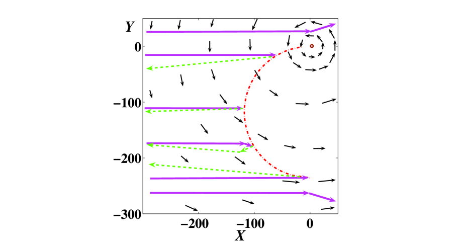
Figure 1: (Color online). Trajectories of excitations with initial momentum ${\bf\Pi}_{0}=(1.0001,0)$ and initial position $(X_{0},Y_{0})$ with $X_{0}=-10^{4}$ for different values of $Y_{0}$ in the presence of a single (positive) vortex at the origin (marked by the dot). The (anticlockwise) superfluid velocity field of the vortex is indicated by arrows. Quasiparticles trajectories are solid (purple) lines, quasiholes trajectories are dashed (green) lines. The dashed-dotted (red) curve denotes the locus of Andreev reflection.

The initial conditions at $\tau=0$ for our calculations are the following. The initial momentum is ${\bf\Pi}_{0}=(1.0001,~{}0)$ and corresponds to a quasiparticle moving in the $x$ direction with energy $E=\Delta_{0}+k_{B}T$ for temperature $T\approx 0.1T_{c}$. The initial position is $(X_{0},Y_{0})$ with $X_{0}=-10^{4}$, far away from the vortex. We study the trajectory of the quasiparticle as a function of $Y_{0}$, which plays the role of impact parameter. Fig. 1 shows results for some typical values of $Y_{0}$. We distinguish three cases:

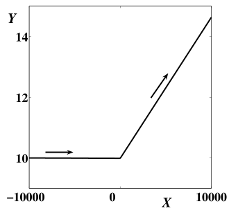
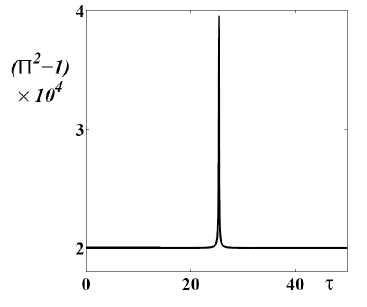
Figure 2: Left: trajectory of the quasiparticle with initial momentum ${\bf\Pi}_{0}=(1.0001,\,0)$ and position $(X_{0},\,Y_{0})=(-10^{4},\,10)$ in the presence of a single anticlockwise vortex at the origin. The arrows indicate the direction of motion. Right: plot of $\Pi^{2}-1$ vs time $\tau$ corresponding to the left part of the figure; note that the quasiparticle remains a quasiparticle.

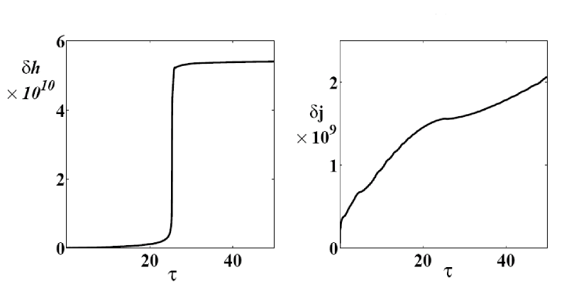
Figure 3: Plot of relative energy variation $\delta h=(H-H_{0})/H_{0}$ vs time $\tau$ (left) and relative angular momentum variation $\delta j=(J-J_{0})/J_{0}$ (right) corresponding to Fig. 2.

Case 1: For $Y_{0}\geq 0$ we have no reflection, in agreement with previous work Nugzar . For example, Fig. 2 (left) shows the quasiparticle’s trajectory for $Y_{0}=10$; Fig. 2 (right) shows that $\Pi^{2}-1$ remains positive at all times $\tau$, which means that the quasiparticle retains its nature of quasiparticle. Fig. 3 confirms that our numerical method conserves energy and angular momentum very well. The left hand side of Fig. 3 shows that the relative error in the energy, $\delta h(\tau)=(H(\tau)-H_{0})/H_{0}$, where $H_{0}$ is the initial energy, is less than $6\times 10^{-10}$; the right hand side of Fig. 3 shows that the relative error in computing the angular momentum, $\delta j(\tau)=(J(\tau)-J_{0})/J_{0}$, where $J_{0}$ is the initial angular momentum, is less than $2.5\times 10^{-9}$.

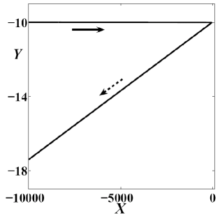
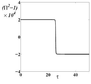
Figure 4: Left: trajectory of quasiparticle with initial momentum ${\bf\Pi}_{0}=(1.0001,\,0)$ and position $(X_{0},\,Y_{0})=(-10^{4},-10)$ in the presence of a single anticlockwise vortex at the origin. The arrows indicate the direction of motion. Right: plot of $\Pi^{2}-1$ vs time $\tau$ corresponding to the left part of the figure; note that the quasiparticle becomes a quasihole.

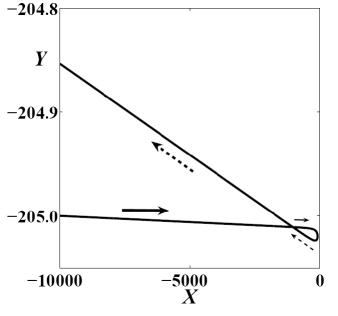
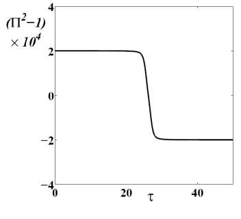
Figure 5: Left: trajectory of the quasiparticle with initial momentum ${\bf\Pi}_{0}=(1.0001,\,0)$ and position $(X_{0},\,Y_{0})=(-10^{4},\,-205)$ in the presence of a single anticlockwise vortex at the origin. The arrows indicate the direction of motion. Right: plot of $\Pi^{2}-1$ vs time $\tau$ corresponding to the left part of the figure; note that the quasiparticle becomes a quasihole.

Case 2: If $Y_{0}<0$ but $|Y_{0}|$ is not too large, the incident quasiparticle is Andreev reflected, as shown for example in Fig. 4 (left) for $Y_{0}=-10$. Fig. 4 (right) shows that $\Pi^{2}-1$ changes sign, thus confirming that, upon reflection, the quasiparticle becomes a quasihole. In this calculation, the numerical errors in conserving energy and angular momentum are $\delta h<8\times 10^{-10}$ and $\delta j<2\times 10^{-9}$ respectively. Fig. 5 shows another Andreev reflection, this time for $Y_{0}=-205$.

In our previous paper Nugzar we determined the distance from the vortex at which, if $Y_{0}<0$, the incident quasiparticle is Andreev reflected; the dashed-dotted (red) curve in Fig. 1 marks this location. It is apparent that there is a maximum value of $|Y_{0}|$ past which a quasiparticle with energy $\epsilon_{p}$ is not Andreev reflected; this value (in our dimensionless units) is approximately equal to $S_{0}=3\pi(\Delta_{0}/\epsilon_{p})^{2}\approx 269$ where we used $\epsilon_{p}=\epsilon_{F}(\Pi^{2}-1)\approx 0.0002\epsilon_{F}$ for $\Pi=1.0001$. We call $S_{0}=269$ the (dimensionless) Andreev shadow of a single vortex to quasiparticles of that particular (dimensionless) momentum $\Pi$.

Case 3: Finally, if $0>-S>Y_{0}$, the quasiparticle’s trajectory is deflected by the vortex but remains a quasiparticle.

IV Vortex-Vortex Pair

The velocity field of two vortices is time-dependent, thus the Hamiltonian of the thermal excitation has no integrals of motion. Unlike the previous case of a single vortex, $H$ and $J$ are not conserved. The only quantity in the problem which is constant is the the distance between the vortices. There are two cases to consider: two vortices of the same circulation (vortex-vortex pair), and two vortices of the opposite circulations (vortex-antivortex pair). This section is concerned with the former.

Two vortices of the same circulation at distance $d$ from each other rotate around a point halfway between them with velocity

$$v_{rot}=\frac{\kappa}{2\pi d}.$$ (24)

In dimensionless variables we have

$$V_{rot}=\frac{1}{2\pi D},~{}~{}~{}~{}~{}D=\frac{d}{\xi_{0}}.$$ (25)

Far from the vortices, the velocity of the quasiparticle can be estimated from Eqs. (15) and (16):

$$\frac{d{\bf R}}{d\tau}\approx 2\lambda^{2}(\Pi^{2}-1){\bf\Pi}.$$ (26)

To get a more clear picture of the problem, it is useful to make the following simple estimates. Away from the vortices, the velocity of the quasiparticle is approximately $400$. If $D=10$, the velocity of the vortices is approximately $0.016$. For a typical timescale of approximately $25$ to $30$ time units, the vortices travel approximately the distance $0.4$ to $0.5$, which means that they rotate about the center of rotation by an angle $\delta\phi\approx 2.3^{o}$ to $3^{o}$. If $D$ is larger than $10$ the vortices move slower and $\delta\phi$ is even smaller. We conclude that, in the first approximation, the vortex system is static to quasiparticles with the momentum ${\bf\Pi}_{0}=(1.0001,\,0)$. However, if ${\bf\Pi}_{0}=(1.00005,\,0)$, in the corresponding time scale the vortices move by a more substantial angle, $\delta\phi\approx 4.5^{o}$ to $6^{o}$. If $D=10$, a significant displacement can be observed for quasiparticles with ${\bf\Pi}_{0}=(1.00002,\,0)$ and the vortex configuration cannot be considered static.

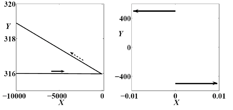
Figure 6: Left: trajectory of the quasiparticle with initial momentum ${\bf\Pi}_{0}=(1.0001,\,0)$ and position $(X_{0},\,Y_{0})=(-10^{4},\,316)$ in the presence of a vortex-vortex pair; the first vortex is at $(Q_{x1},\,Q_{y1})=(0,\,-500)$, and the second vortex is at $(Q_{x2},\,Q_{y2})=(0,\,500)$. The solid arrow indicates the incident quasiparticle, the dashed arrow the reflected quasihole. Right: Directions of motion of the two vortices.

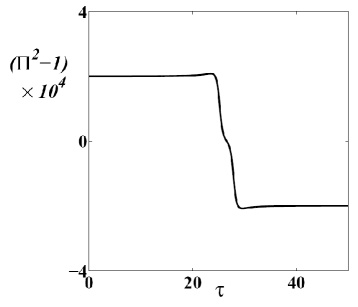
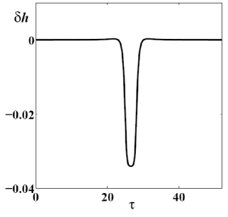
Figure 7: Left: plot of $\Pi^{2}-1$ vs time $\tau$ corresponding to the left part of Fig. 6; note that the quasiparticle becomes a quasihole. Right: plot of relative energy difference $\delta h=(H(\tau)-H_{0})/H_{0}$ vs time $\tau$.

We proceed with our calculations and consider two vortices of the same circulation at distance $D=1000$ from each other, initially located at positions $(Q_{x1},\,Q_{y1})=(0,\,-500)$ and $(Q_{x2},\,Q_{y2})=(0,\,500)$. We integrate the equations of motion of quasiparticles with ${\bf\Pi}_{0}=(1.0001,\,0)$, keeping $X_{0}=-10^{4}$ fixed and varying $Y_{0}$. In this configuration, the relative angle $\theta$ between the direction of the incoming quasiparticle (the $x$ axis) and the line which joins the two vortices (the $y$ axis) is $\theta=90^{o}$. Fig. 6 illustrates the trajectories of the quasiparticle for $Y_{0}=316$ as well as the path of the vortices; Fig. 7 (left) shows that the incident quasiparticle is reflected as a quasihole; since the ${\bf{p}}\cdot{\bf v}_{s}$ term in the Hamiltonian is time-dependent, the energy is not constant during the evolution, as confirmed in Fig. 7 (right). We find that the Andreev shadow of the first vortex of the pair is $S_{1}=290$, slightly more than $S_{0}$ (the Andreev shadow of an isolated stationary vortex), and that the shadow of the second vortex of the pair is $S_{2}=184$, which is slightly less than $S_{0}$. Note that in this case $S_{1}+S_{2}\approx 2S_{0}$.

If the relative angle $\theta$ between the direction of the incoming quasiparticle and the direction between the vortices is reduced from $\theta=90^{o}$ to $\theta=45^{o}$, the Andreev shadow of the first vortex decreases from $S_{1}=290$ to $S_{1}=272$, but the Andreev shadow of the second vortex increases from $S_{2}=184$ to $S_{2}=205$, so that the total shadow $S_{1}+S_{2}$ of the vortex configuration remains approximately equal to twice the shadow $S_{0}$ of a single isolated vortex. For example, if the vortices are located at $(Q_{x1},\,Q_{y1})=(-353,\,-353)$ and $(Q_{x2},\,Q_{y2})=(353,\,353)$, the angle is $\theta=45^{o}$, $S_{1}=272$, $S_{2}=205$, and $S_{1}+S_{2}=477$. If $\theta$ is further reduced from $\theta=45^{o}$ to $14.1^{o}$, the total shadow of both vortices increases and reaches its maximum size: $S_{1}=263$, $S_{2}=242$, and $S_{1}+S_{2}=505$. If $\theta>14.1^{o}$ the two shadows merge, and the two vortices screen each other. If $\theta=0^{o}$ then $S_{1}+S_{2}=251$ only.

Qualitatively, the same behaviour is observed if the distance between the vortices is even smaller, e.g. $D=100$. If the angle between the direction of motion of the excitation and the direction of the line through the vortices is $\theta=90^{o}$, the shadow of the first vortex at $(Q_{x1},\,Q_{y1})=(0,\,50)$ is only $S_{1}=44.7$ (significantly smaller than $S_{0}$) and the shadow of the second vortex at $(Q_{x2},\,Q_{y2})=(0,\,-50)$ is $S_{2}=443.3$ (significantly larger than $S_{0}$), and the total shadow is $S_{1}+S_{2}=488$. If $\theta$ is reduced the two shadows merge when $\theta\approx 75^{o}$; at this angle $S_{1}+S_{2}=526$. At $\theta=45^{o}$, the total shadow is $S_{1}+S_{2}=510$, and at $\theta=0^{o}$ $S_{1}+S_{2}=469$.

What happens if $D$ is further reduced? Consider for simplicity the angle $\theta=90^{o}$: for large $D$ the two vortices have independent shadows (one reduced in size, the other increased in size). By decreasing the distance between the vortices the shadows approach each other; for distances $D\lesssim 16$ they merge and the vortex configuration has a single shadow independent of $\theta$, as if it were a single vortex of strength approximately equal to $2\kappa$.

V Vortex-antivortex pair

A vortex and an antivortex, set at distance $D$ from each other, move through the fluid with (dimensionless) translational velocity

$$V_{tran}=\frac{1}{2\pi D},~{}~{}~{}~{}~{}D=\frac{d}{\xi_{0}}.$$ (27)

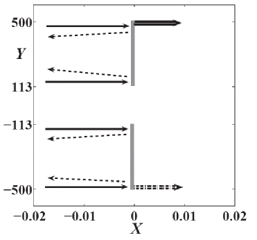
Figure 8: Andreev reflection of quasiparticles from the vortex-antivortex pair travelling in the same direction. The solid lines denote quasiparticles travelling left to right; the dotted lines denote the reflected quasiholes. The solid double arrow denotes the path of the vortex, initially located at $(Q_{x1},\,O_{y1})=(0,\,500)$ with separation $D=1000$; the dash-dotted double arrow denotes the path of the antivortex, initially located at $(Q_{x2},\,Q_{y2})=(0,\,-500)$. The thick vertical grey lines denote the shadows of the vortices.

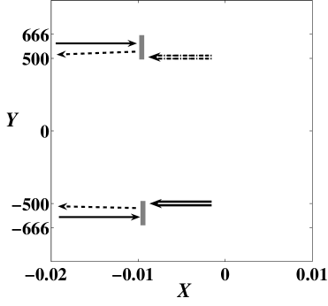
Figure 9: Andreev reflection of quasiparticles from the vortex-antivortex pair, with separation $D=1000$, travelling in the opposite direction. The solid lines denote quasiparticles travelling left to right; the dotted lines denote the reflected quasiholes. The dash-dotted double arrow denotes the path of the vortex, initially located at $(Q_{x1},\,Q_{y1})=(0,\,-500)$; the solid double arrow denotes the path of the antivortex, initially located at $(Q_{x2},\,Q_{y2})=(0,\,500)$. The thick vertical grey lines denote the shadows of the vortices. Note that the shadows are much smaller than in Fig. 8.

The same estimates which we have made at the beginning of the previous section apply. As before, we consider quasiparticles with initial momentum ${\bf\Pi}_{0}=(1.0001,\,0)$ and initial position $(X_{0},\,Y_{0})$ with $X_{0}=-10^{4}$ fixed and varying $Y_{0}$. Firstly we consider the case in which the vortex-antivortex pair and the quasiparticle move in the same direction. Let the positive (anticlockwise) vortex be located at $(Q_{x1},\,Q_{y1})=(0,\,500)$ and the negative (clockwise) vortex be at $(Q_{x2},\,Q_{y2})=(0,\,-500)$, with $D=1000$ the separation between the vortices. We find that the total shadow of the vortex configuration is $S_{1}+S_{2}=774$, as shown in Fig. 8. Secondly we consider the case in which the vortex-antivortex pair and the quasiparticle move in the opposite directions, letting the positive vortex be at $(Q_{x1},\,Q_{y1})=(0,\,-500)$ and the negative vortex at $(Q_{x2},\,Q_{y2})=(0,\,500)$: we find that the total shadow is greatly reduced: $S_{1}+S_{2}=332$, as shown in Fig. 9. In both cases, during the timescale of the calculation, the vortex pair moves by only $0.01$. We conclude that the relative motion of vortices and excitations has a strong effect on the shadow.

Now we examine the dependence of the Andreev reflection on $D$. Firstly, we consider the case in which the quasiparticle and the vortex pair move in the same direction. We said that, at $D=1000$, the total shadow is $S_{1}+S_{2}=774$. If we reduce $D$, the total shadow increases, and at the value $D=940$ the two shadows merge into a single shadow of size $S_{1}+S_{2}=940$. Upon further reduction of $D$, the total shadow decreases; for example, when $D=100$, $S_{1}+S_{2}=122$, and when $D=10$ we have $S_{1}+S_{2}=34$. Secondly, we consider the case in which the quasiparticle and the vortex pair move in opposite directions. We have said that if $D=1000$ the total shadow is only $S_{1}+S_{2}=332$. If $D$ decreases, $S_{1}+S_{2}$ decreases too: at $D=100$ and $D=10$ we have $S_{1}+S_{2}=222$ and $88$ respectively. We conclude that, independently of $D$, the total shadow of a vortex pair travelling in the opposite direction of the quasiparticle is about half that of a vortex pair travelling in the same direction.

The shadow of the vortex-antivortex pair also depends on the angle $\alpha$ between the direction of propagation of the quasiparticle and the direction of motion of the vortex-antivortex pair. Consider a vortex-antivortex pair of separation $D=100$. We have already seen that if $\alpha=0$ (vortex pair moving in the same direction as the quasiparticle), then $S=122$. If the positive vortex is at $(35.33,\,35.33)$ and the negative vortex is at $(-35.33,\,-35.33)$, the angle is $\alpha=-45^{o}$ and the shadow increases to $168$. If the positive vortex is at $(50,\,0)$ and the negative vortex at $(-50,\,0)$, the angle is $\alpha=-90^{o}$ and the shadow increases further to $S=233$. Finally, as said before, if the positive vortex is at $(0,\,-50)$ and the negative vortex is at $(0,\,50)$ (the vortex pair moving in the direction opposite to that of the quasiparticle), then $\alpha=-180^{o}$ and $S=222$.

VI Many vortices

We assume again that the quasiparticle has initial momentum ${\bf\Pi}_{0}=(1.0001,\,0)$ and initial position $(X_{0},\,Y_{0})$ with $X_{0}=-10^{4}$; we vary $Y_{0}$ and determine the total shadow of some simple vortex configurations.

In the first numerical experiment we initially place five vortex points in the square $-250\leq X\leq 250$, $-250\leq Y\leq 250$. More precisely, the initial positions of the vortices are $(-250,\,0)$, $(0,\,0)$, $(250,\,0)$, $(250,\,-250)$ and $(-250,\,-250)$.

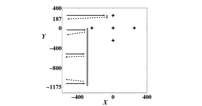
Figure 10: Trajectories of quasiparticles (solid lines), of initial momentum ${\bf\Pi}_{0}=(1.0001,\,0)$ and initial position $(-10^{4},\,Y_{0})$ for varying $Y_{0}$, interacting with a configuration of five positive vortices (denoted by crosses) initially located at $(-250,\,0)$, $(0,\,0)$, $(250,\,0)$, $(250,\,-250)$ and $(-250,\,-250)$. The reflected quasiholes are indicated as dotted lines; the shadow of the vortex configuration is the thick grey line.

If the vortices have the same (positive) polarity, they rotate around each other, forming the 2-dimensional equivalent of a vortex bundle of total circulation $5\kappa$; we find (see Fig. 10) that the total shadow of the vortex configuration is $S=1238$, which is less than five times the shadow of five individual vortices.

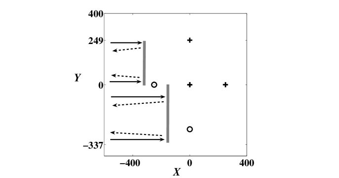
Figure 11: Trajectories of quasiparticles (solid lines), of initial momentum ${\bf\Pi}_{0}=(1.0001,\,0)$ and initial position $(-10^{4},\,Y_{0})$ for varying $Y_{0}$, interacting with an initial configuration of three positive vortices (denoted by crosses) located at $(0,\,0)$, $(250,\,0)$ and $(0,\,250)$ and two negative vortices located at $(-250,\,0)$ and $(0,\,-250)$ denoted by circles. The reflected quasiholes are indicated as dotted lines; the shadow of the vortex configuration is the thick grey line.

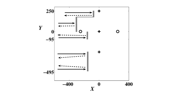
Figure 12: Trajectories of quasiparticles (solid lines), of initial momentum ${\bf\Pi}_{0}=(1.0001,\,0)$ and initial position $(-10^{4},\,Y_{0})$ for varying $Y_{0}$, interacting with an initial configuration of three positive vortices (crosses) located at $(0,\,0)$, $(0,\,250)$ and $(0,\,-250)$ and two negative vortices (circles) located at $(250,\,0)$ and $(-250,\,0)$. The reflected quasiholes are indicated as dotted lines; the total shadow of the vortex configuration, $S=589$, is the thick grey line. Note the gap in the shadow within the interval $-95\leq Y_{0}\leq 0$.

If we change the sign of some of the vortices, the total shadow which is cast changes dramatically. For example, let the vortices at $(0,\,0)$, $(0,\,250)$ and $(250,\,0)$ be positive, and the vortices at $(-250,\,0)$ and $(0,\,-250)$ be negative. The net circulation is now $\kappa$ and the total shadow is $S=585$ (see Fig. 11), which is much less than the previous value, but still more than the shadow of a single isolated vortex. A similar value of the total shadow, $S=589$, is obtained if the positive vortices are at $(0,\,0)$, $(0,\,250)$, $(0,\,-250)$ and the negative vortices are at $(-250,\,0)$, $(250,\,0)$, which corresponds to the same total circulation $\kappa$ as before, see Fig. 12.

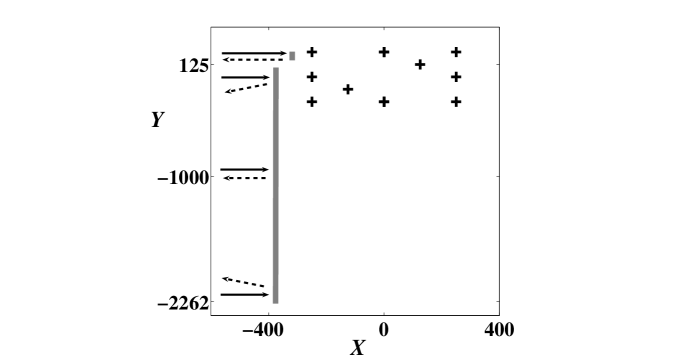
Figure 13: Schematic trajectories of quasiparticles (solid arrows), of initial momentum ${\bf\Pi}_{0}=(1.0001,\,0)$ and initial position $(-10^{4},\,Y_{0})$ for varying $Y_{0}$ interacting with an initial configuration of ten positive vortices (crosses) located at $(-250,\,0)$, $(-250,\,250)$, $(-125,\,-125)$, $(0,\,-250)$, $(0,\,250)$, $(125,\,125)$, $(250,\,-250)$, $(250,\,0)$ and $(250,\,250)$. The reflected quasiholes are indicated as dashed arrows. The thick grey vertical lines indicate the shadows of the vortices. The total shadow is $S=2445$.

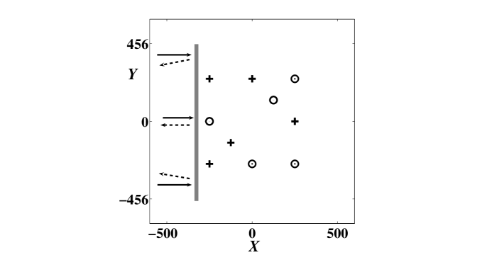
Figure 14: Schematic trajectories of quasiparticles (solid arrows), of initial momentum ${\bf\Pi}_{0}=(1.0001,\,0)$ and initial position $(-10^{4},\,Y_{0})$ for varying $Y_{0}$, interacting with an initial configuration of five positive vortices (crosses) located at $(-250,\,-250)$, $(-250,\,250)$, $(-125,\,-125)$, $(0,\,250)$, and five antivortices (circles) at the $(-250,\,0)$, $(0,\,-250)$, $(125,\,125)$, $(250,\,-250)$ and $(250,\,250)$. The reflected quasiholes are indicated as dashed arrows. The thick grey vertical line indicates the shadow of the vortices. The total shadow is $S=902$.

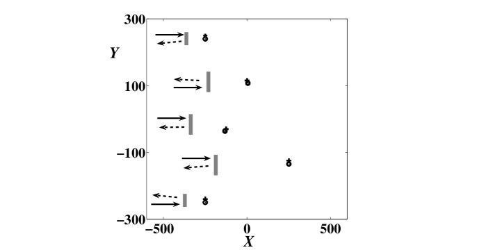
Figure 15: Schematic trajectories of quasiparticles (solid arrows), of initial momentum ${\bf\Pi}_{0}=(1.0001,\,0)$ and initial position $(-10^{4},\,Y_{0})$ for varying $Y_{0}$, interacting with an initial configuration of five vortex-antivortex pairs located at: vortex at $(-250,\,-240)$ and antivortex at $(-250,\,-250)$, vortex at $(-250,\,250)$ and antivortex at $(-250,\,-240)$, vortex at $(-125,\,-30)$ and antivortex at $(-132,\,-36)$, vortex at $(0,\,115)$ and antivortex at $(5,\,107)$, vortex at $(250,\,-125)$ and antivortex at $(250,\,-135)$. (Note that the distance between the vortex and the antivortex in each pair is 10 non-dimensional units and cannot be distinguished on this figure.) The schematic reflected quasiholes are indicated as dashed arrows. The thick grey vertical lines indicate the shadows of the vortices. The total shadow is $S=209$.

In the second numerical experiment we increase the vortex density and place ten vortices (twice as many as before) in the same square $-250\leq X\leq 250$, $-250\leq Y\leq 250$. We consider three cases: (i) ten vortices of the same polarity (total circulation $10\kappa$, see Fig. 13), which yields the total shadow $S=2445$ (about twice the shadow of a bundle of five vortices); (ii) five vortices and five antivortices (total circulation is zero, see Fig. 14), which yields $S=902$; (iii) five vortex-antivortex pairs (total circulation zero, see Fig. 15), which yields $S=209$.

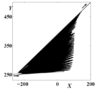
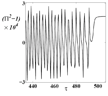
Figure 16: Left: trajectory of the quasiparticle with initial momentum ${\bf\Pi}_{0}=(1.0001,\,0)$ and position $(X_{0},\,Y_{0})=(-10^{4},\,10)$ in the presence of five positive vortices and five negative vortices as in Fig. 14. Note the multiple reflections before the particle’s escape from the vortex region. The arrows indicate the direction of motion. Right: plot of $\Pi^{2}-1$ vs time $\tau$ corresponding to a small time interval just before the escape. Note that the quasiparticle turns into a quasihole many times, before escaping as a quasiparticle.

We have found that it is possible that, upon impinging on complex vortex configurations, quasiparticles experience multiple reflections, which can be classical, Andreev, or both. An example of multiple Andreev reflection is shown in Fig. 16.

VII Conclusions

In conclusion, the above numerical experiments with simple vortex configurations show that partial screening takes place. The total Andreev shadow of a vortex system is not necessarily the sum of the shadows of individual vortices, and depends not only on the distance but also on the relative orientation between quasiparticles and vortex motion. This does not mean that the interpretation given to recent experiments is incorrect. It is possible that, for a large, random vortex system, the partial screening effects which we have found average out. If this is the case, screening effects can be taken into account by introducing a prefactor probably of order one for the total shadow, hence for the vortex line density which is inferred. Numerical investigations in 3-dimensions with realistic vortex line density are needed.

How random are vortex configurations of current experiments? Probably only the recently discovered Golov2008 ; Walmsley ultraquantum regime is truly random. Homogeneous isotropic turbulence contains coherent vortex structures Farge ; Sultan ; Kivotides and is organized in scales with different energy per scale. On the other hand, provided we are interested only in large scale properties averaged over a large region, such as the total vortex length, the partial screening effects can be accounted as said above.

The situation is very different when we move to rotating turbulence Tsubota ; Eltsov2008 ; Eltsov2006 and inhomogeneous turbulence, particularly if there are turbulent fronts. In these cases there is large scale anisotropy, and the Andreev reflection technique must be used with more care than we used to. The good news is that, by combining Andreev reflection measurements in different directions and numerical calculations such as those we have presented, it should be possible to gain more information about the geometry and the anisotropy of the turbulence.

Our results also indicate that the problem of interaction between rotons and quantized vortices in ⁴He Samuels , leading to calculation of the mutual friction, should be reconsidered in view of possible screening effects analyzed above in Secs. IV and V.

VIII Acknowledgments

N.S. was supported by the Georgian National Science Foundation Grant No. GNSF/ST06/4-018. We are grateful to S. N. Fisher for stimulating discussions.

References

- (1) C. F. Barenghi, R. J. Donnelly, and W. F. Vinen (Eds.), Quantised Vortex Dynamics And Superfluid Turbulence, Springer Verlag (2001).
- (2) S. I. Davis, P. C. Hendry, and P. V. E. McClintock, Physica B 280, 43 (2000).
- (3) S. N. Fisher, A. J. Hale, A. M. Guénault, and G. R. Pickett, Phys. Rev. Lett. 86, 244 (2001).
- (4) C. F. Barenghi and D. C. Samuels, Phys. Rev. Lett. 89, 155302 (2002).
- (5) W. F. Vinen and J. J. Niemela, J. Low Temp. Phys. 128, 167 (2002), and Erratum 129, 213 (2002).
- (6) T. Araki, M. Tsubota, and S. K. Nemirovskii, Phys. Rev. Lett. 89, 145301 (2002).
- (7) C. Nore, M. Abid and M. E. Brachet, Phys. Rev. Lett. 78, 3896 (1997).
- (8) M. Kobayashi and M. Tsubota, Phys. Rev. Lett. 94, 065302 (2005).
- (9) W. F. Vinen, Phys. Rev. B 64, 134520 (2001).
- (10) W. F. Vinen, M. Tsubota, and A. Mitani, Phys. Rev. Lett. 91, 135301 (2003).
- (11) C. F. Barenghi, N. G. Parker, N. P. Proukakis, and C. S. Adams, J. Low Temp. Phys. 138, 629 (2005);
- (12) M. Leadbeater, T. Winiecki, D. C. Samuels, C. F. Barenghi and C. S. Adams, Phys. Rev. Lett. 86, 1410 (2001).
- (13) D. Kivotides, J. C. Vassilicos, D. C. Samuels, and C. F. Barenghi, Phys. Rev. Lett. 86, 3080 (2001).
- (14) V. S. L’vov, S. V. Nazarenko, and G. E. Volovik, JETP Lett. 80, 479 (2004).
- (15) E. Kozik and B. Svistunov, Phys. Rev. Lett. 92, 035301 (2004).
- (16) P. M. Walmsley, A. I. Golov, H. E. Hall, A. A. Levchenko, and W. F. Vinen, Phys. Rev. Lett. 99, 265302 (2007).
- (17) P. M. Walmsley and A. I. Golov, arXiv:0802.2444v1 (2008).
- (18) G. E. Volovik, JETP Lett. 78, 533 (2003).
- (19) P.-E. Roche, P. Diribarne, T. Didelot, O. Francais, L. Rousseau, and W. H. Willaime, Europhys. Lett. 77, 66002 (2007).
- (20) P.-E. Roche and C. F. Barenghi, Europhys Lett. 81, 36002, 2008.
- (21) D. I. Bradley, S. N. Fisher, A. M. Guénault, R. P. Haley, S. O’Sullivan, G. R. Pickett, and V. Tsepelin, private communication (2007).
- (22) H. Yano, N. Hashimoto, A. Handa, M. Nakagawa, K. Obara, O. Ishikawa, and T. Hata, Phys. Rev. B 75, 012502 (2007).
- (23) D. I. Bradley, D. O. Clubb, S. N. Fisher, A. M. Guénault, R. P. Haley, C. J. Matthews, G. R. Pickett, V. Tsepelin, and K. L. Zaki, J. Low Temp. Phys. 138, 493 (2005).
- (24) D. I. Bradley, D. O. Clubb, S. N. Fisher, A. M. Guénault, R. P. Haley, C. J. Matthews, G. R. Pickett, V. Tsepelin, and K. Zaki Phys. Rev. Lett. 95, 035302 (2005).
- (25) L. Skrbek, in Vortices and Turbulence at Very Low Temperatures, edited by C. F. Barenghi and Y. A. Sergeev, CISM Courses and Lectures, Vol. 501 (Springer, Wien New York, 2008), pp. 91-137.
- (26) C. F. Barenghi, A. V. Gordeev, and L. Skrbek, Phys. Rev. E 74, 026309 (2006).
- (27) C. E. Swanson, C. F. Barenghi, and R. J. Donnelly, Phys. Rev. Lett. 50, 190 (1983).
- (28) M. Tsubota, T. Araki, and C. F. Barenghi, Phys. Rev. Lett. 90, 205301 (2003).
- (29) V. B. Eltsov, A. P. Finne, R. Hänninen, J. Kopu, M. Krusius, M. Tsubota, and E. V. Thuneberg, Phys. Rev. Lett. 96, 215302 (2006).
- (30) V. B. Eltsov, R. de Graaf, R. Hänninen, M. Krusius, R. F. Solntsev, V. S. L’vov, A. I. Golov, and P. M. Walmsley, ArXiv:0803.3225v1 (2008).
- (31) C.F. Barenghi, Physica D 237, 2195 (2008).
- (32) T. Zhang and S. W. Van Sciver, Nat. Phys. 1, 36 (2005).
- (33) M. S. Paoletti, M. E. Fisher, K. R. Sreenivasan, and D. P. Lathrop, Phys. Rev. Lett. 101, 154501 (2008).
- (34) D. I. Bradley, S. N. Fisher, A. M. Guénault, M. R. Lowe, G. R. Pickett, A. Rahm, and R. C. V. Whitehead, Phys. Rev. Lett. 93, 235302 (2004).
- (35) S.N. Fisher, in Vortices and Turbulence at Very Low Temperatures, edited by C. F. Barenghi and Y. A. Sergeev, CISM Courses and Lectures, Vol. 501 (Springer, Wien New York, 2008), pp. 177-257.
- (36) D. C. Samuels and R. J. Donnelly, Phys. Rev. Lett. 65, 187 (1990).
- (37) N. B. Kopnin and V. E. Kravtsov, Sov. Phys. JETP 44, 861 (1976).
- (38) M. Stone, Phys. Rev B 54, 13222 (1996).
- (39) G. E. Volovik, The Universe in a Helium Droplet (Clarendon, Oxford, 2003).
- (40) C. F. Barenghi, Y. A. Sergeev, and N. Suramlishvili, Phys. Rev. B 77, 104512 (2008)
- (41) J.C. Wheatley, Rev. Mod. Phys. 47, 415 (1975).
- (42) J. Bardeen, R. Kummel, A. E. Jacobs, and L. Tewordt, Phys. Rev. 187, 556 (1969).
- (43) T. Tsuneto, Superconductivity and Superfluidity (Cambridge University Press, Cambridge, England, 1998).
- (44) N. A. Greaves and A. J. Leggett, J. Phys. C (Solid State Physics) 16, 4383 (1983).
- (45) J. M. Sanz-Serna and M. P. Calvo, Numerical Hamiltonian Problems (Chapman & Hall, London, 1994).
- (46) L. F. Shampine and M. W. Reichelt, SIAM J. Sci. Comput. 16, 1 (1997).
- (47) M. Farge, G. Pellegrino, and K. Schneider, Phys. Rev. Lett. 87, 054501 (2001)
- (48) S. Alamri, A. Y. Youd and C. F. Barenghi, arXiv:0809.4746v1 (2008), to be published in Phys. Rev. Letters.
- (49) D. Kivotides, Phys. Rev. B 76, 054503 (2007).