Pulsars as Fantastic Objects and Probes

Abstract

Pulsars are fantastic objects, which show the extreme states of matters and plasma physics not understood yet. Pulsars can be used as probes for the detection of interstellar medium and even the gravitational waves. Here I review the basic facts of pulsars which should attract students to choose pulsar studies as their future projects.

Keywords: Pulsars, ISM, Gravitational waves

1 Pulsars: General Introduction

Pulsars are sending us pulses – we can receive these pulses in radio bands. A small number of pulsars also emit high energy radiation in optical and X-ray or even $\gamma$-ray bands. Here let me discuss the radio pulsars, and leave the high energy emission and its explanation to Prof. Qiao in this volume.

After the first pulsar discovered by Hewish et al. hbp+68 in 1968, it was soon realized that they are rotating neutron stars gold68 ; pac68 with a diameter of only 20 km but extremely high density ($10^{15}$g cm^-3) and extremely strong magnetic fields ($10^{8}$ to $10^{14}$ G). Because of revealing of this new state of matter in the universe, the pulsar discovery was awarded the Nobel Prize in 1974 in physics.

Pulsars take birth in supernova explosion, which is evident from the young pulsars and supernova remnants associations kas98 . For example, the Vela pulsar is located in the center of Vela nebula, the Crab pulsar is acting as the heart of Crab nebula. Pulsars get high velocity (a few 100 km s^-1) hllk05 ; wlh06 in the explosion so that pulsars are running away quickly from their birthplace, even about half pulsars have escaped from our Galaxy in last 100 Myr sh04 .

The broadband radio emission of pulsars leaves from the emission region almost simultaneously. However, after these signals pass through the interstellar medium (ISM), the radio waves at a lower frequency, $\nu_{1}$, in GHz, come later than these at a higher frequency $\nu_{2}$, with a time delay of

$$dt=4.15\left({1\over\nu_{1}^{2}}-{1\over\nu_{2}^{2}}\right)DM~{}~{}~{}{\rm ms},$$ (1)

where $DM$ is known as the dispersion effect from the ionized gas in the ISM along the path from a pulsar to us, given by

$$DM=\int_{0}^{D}n_{e}dl~{}~{}~{}\mbox{pc~{}cm${}^{-3}$},$$ (2)

where $n_{e}$ is the electron density in units of cm^-3 and $D$ the distance from observer to pulsar in pc. In Fig. 1 (left panel), we have plotted the signals received in each frequency channel as function of pulse phase. It is evident that the signals at low frequency are delayed in arrival time compared to those at high frequencies. After making the delay corrections and adding the channels we get the pulse profile (see Fig. 1 right panel).

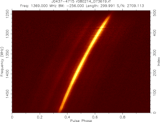
Figure 1: The dispersion of pulsed signals – the example is observation of PSR J0437-4715 (left). The dedispersion and adding signals from all frequency channels gives a strong and stable profile (right). Data is obtained by the author with Parkes telescope.

How to find pulsars? Because a pulsar have a very accurate period – the period change due to slow-down is small enough in half an hour, one can make Fourier transform of the recorded power, and found the period in the power-spectrum. Nowadays, there are many terrestrial radio frequency interferences (RFI) which look like pulsar signals. However, these RFI normally show the maximum power at zero dispersion. Therefore, when radio power from many frequency channels is recorded, only after the power from all channels are properly de-dispersed the pulsar signal should show the maximum power. Therefore, here are several steps to find a new pulsar: 1) record signals in time series at many frequency-channels; 2) de-disperse the channel signals with many trial DM and add all channels together to get one time series for each trial DM; 3) search for the periodicity from each dedispersed time series. Because most pulsars have only narrow pulses, the power-spectrum should show not only the primary pulsar rotation frequency, but also its harmonics. Often the harmonics are added together to enhance the searching signal-to-noise ratio; 4) verify the dedispersed pulse by searching for the best detection signal-to-noise ratio in the 2-D parameter space around the proposed $P$ and $DM$ and then folding data in the right period $P$ and $DM$; 5) finally re-observe again in this sky position and search the pulse again around the proposed $P$ and $DM$. If the pulse can be found in the same DM but slightly evolved period, then a pulsar is definitely found! See mlc+01 ; cfl+06 for the pulsar searching strategy.

Up to now, about 1800 pulsars have been discovered mht+05 , including some discovered using the GMRT fgr+04 ; jmk+07 . Most of pulsars are in our Milky way Galaxy, and only about 20 were discovered from extensive searches of nearby galaxies, the Large and Small Magellanic clouds. Pulsars have a period of 1.3 ms to $\sim$10 s. Some very fast rotating pulsars, so-called millisecond pulsars, have a period of only some milliseconds but very stable and very small period derivatives. From measurements of binary pulsars, it has been established that neutron stars normally have a mass pr06 about 1.4 solar mass ($M_{\odot}$) though some are heavier (probably up to 2 $M_{\odot}$) and some are lighter (1.2 $M_{\odot}$).

Here are pulsar books I would like to recommend to readers: 1). “Handbook of Pulsar Astronomy”, by D. Lorimer and M. Kramer lk05 , published by the Cambridge University Press (2005), contains many up-to-dated material of pulsar studies; 2) “Pulsar Astronomy” by A. Lyne & F. Graham-Smith lg06 , also published by the Cambridge University Press (2006), is an excellent text book for graduate students, covering all aspects of pulsar astrophysics.

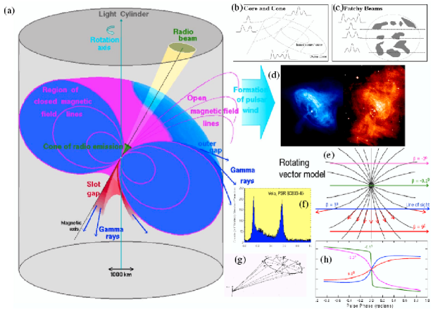
Figure 2: The magnetosphere and radiation of neutron stars: (a) the particles are accelerated in the inner gap, outer gap or the slot gap, and radio emission beams out near the magnetic poles. The radio beam is not uniformly illuminated but maybe more bright in (b) conal regions or (c) randomly in patches. The outflowing particles can form the pulsar wind nebula. The polarization of the radio emission depends on (e) the magnetic field planes – when the (g) line of sight impacts the beam, the observed polarization angles show variations in the (h) “S-shaped” curves. This demonstration is composed by using the artwork produced by Drs. B. Link, D. Lorimer, A. Harding, G.J. Qiao, as well as (d) the Chandra and HST images of the Crab pulsar nebula, and (f) the $\gamma$-ray profile of the Vela pulsar.

2 Pulsar emission

Radio emission from pulsars is generated in pulsar magnetosphere. We define the boundary of this magnetosphere by the light-cylinder, e.g. at the radius where the rotation speed is equal to the light speed. The particles, i.e. positrons and electrons, are accelerated along the magnetic fields above polar cap or the outer gap. These particles radiate gan04 so that we can see the emission in radio and high energy band. However, it is not clear what physical processes are involved for the particles to radiate. Pulsar wind or wind nebula sla08 can be formed if particles flow out through the open magnetic field lines passing through the light-cylinder.

It is the rotation that provides the energy source for pulsar emission and particle outflowing. One can calculate the braking torque due to magnetic dipole radiation, which finally result in $\dot{\mu}=-K\mu^{n}$, here the $\mu$ is the rotation frequency of the neutron star, and the $n$ is the braking index which theoretically should be equal to 3. However, the measurements show that it is usually significantly smaller than 3, which implies yxz07 that other reasons are also consuming the rotation energy, e.g. pulsar wind. Otherwise, magnetic fields may evolve. The smaller index means that the magnetic fields may be growing lz04 . In Fig. 2, I provide an over view on pulsars, and models in understanding their action.

2.1 Pulse profiles and emission beam

Pulsars emit broadband radio waves. We receive these signals when the emission beam is sweeping towards us. The line of sight impacts the emission beam so that we see a pulse profile. Now it is clear that 1) the average pulse profiles are very stable, except for a few pulsars with precession sls00 ; wt02 ; 2) profiles are the finger-prints of pulsars which differ from each other. Most pulsar profiles have one or two or three distinctive components or peaks, a small number of pulsars have 4 or 5, and occasionally more than 10 components mh04 . Some components are difficult to be identified, but can be revealed by multi-Gaussian fitting wgr+98 or “window-threshold technique” gg01 ; 3) these profiles vary with frequency, and each component has some-how independent spectral index mh04 , although in general pulsars have very steep spectrum mkkw00 ; 4) some pulsars have a main pulse and an interpulse, separating about $180^{\circ}$ in the rotation phase, which look like the emission from the two opposite magnetic poles; 5) Some pulsars show profiles in two or three modes, which is so-called “mode-changing”. Some pulsars even switch off their emission for sometime, which is called “nulling” wmj07 .

Figure 3: The polarization profile of PSR J2124-3358 at 659 MHz (top panel) shows more than 12 distinguishable components, each with different fraction of linear (dash line) and circular polarization (lower solid line). Comparison of profiles at 659 MHz and 1327 MHz (lower panel) show that the spectrum varies against rotation phase. This is an extraordinary profile (data from mh04 ) and usually pulsars are not so complicated – see Fig.4.

It is naturally understandable that the profile peaks indicate the bright parts of the emission beam. That is to say, the pulsar emission beam is not uniformly illuminated, some parts brighter, some fainter. The line of sight only impacts one slice of beam for a given pulsar, so it is not possible to know the whole beam of any pulsar, except that one can fly in space (!) and observe a pulsar in different lines of sight with respect to its rotational axis! However, based on profiles of many pulsars, the emission beam has been suggested ideally to consist of one core and nested cones ran83 ; gg01 . This image gained some good support from the observational fact of the widening of the double profiles at lower frequencies tho91 . This is so-called “radius-frequency mapping”, which is explained as the emission comes from a pair cuts of the “outer cone” formed in the open dipole magnetic fields. However, if all peak emission comes from cones, how many cones are needed to explain more than 10 components of some pulsars? Can these emission cones be really formed above the magnetic polar caps? This problem can be eased in the so-called “patchy beam” model lm88 , where the emission comes from many bright parts of a beam. If the slices of emission beams of all pulsars are put together, one can not see distinct cones hm01 .

In fact, the averaged pulse profiles can only be used to reveal emission geometry or brightness distribution of the emission beam. A large amount of information on the emission process can be obtained from observations of individual pulses dr99 ; dr01 . It has been established that for pulsars with drifting subpulses, some emission zones is stably circulating around the magnetic axis of some pulsars with remarkably organized configuration. A detailed modeling hints that the imagined emission cones are patchy! To my understanding, “the patchy cones” seems to be the best description of the characteristics of pulsar emission beam: the cones only roughly define the emission region in the magnetosphere and “patches” are related to the non-random but preferred bunches of field lines for generation of emission spots which are probably physically related to sparking near the polar cap. This idea is similar but different from the idea of “window+sources” proposed by Manchester in 1995 man95 .

2.2 Polarization

Pulsars are the strongest polarized radio sources in the universe. Almost 100% linear polarization is detected (see Fig. 4) for the whole or a part of profiles of some pulsars wmlq93 ; mhq98 ; wcl+99 . In fact, it is the polarization angle sweeping of the Vela pulsar that leads to the famous “rotating vector model” proposed by Radhakrishnan and Cooke in 1969 rc69 , which solidly established that the radio emission comes from region not far away from the magnetic poles of the neutron stars, and the observed polarization angle is related (either parallel or perpendicular) to the plane of magnetic field lines, which should have a “S”-shape (see PSR J2048$-$1616).

Assuming magnetic fields of pulsars are dominated by the dipole fields, then one can determine the emission geometry from the polarization observations ran83 . The maximum polarization angle swept rate gives the information on the smallest impact angle of the line-of-sight from the magnetic axis lm88 . After classification of pulsar profiles, Rankin has made extensive efforts to pin down the emission regions, by calculating the geometrical parameters for various types of pulsars ran83 ; ran90 ; ran93a ; ran93b . The geometrical parameters of a large number of pulsars were also calculated by Gould & Lyne gl98 . From the phase shift between the pulse center and the largest sweep rate of polarization angle curve, the emission latitude can be estimated bcw91 ; gan05 .

The polarization angle curves often are not smooth but have some jumps (see PSR J1932+1059 in Fig. 4). When the polarization data samples of individual pulses are plotted against the phase bins, the orthogonal polarization modes can be solidly identified man75 ; crb78 ; scr+84 ; scm+84 . Several possible origins of the orthogonal polarization modes have been suggested. These orthogonally polarized modes may reflect the eigenmodes of the magneto-active plasma in the open magnetic field lines above the pulsar polar cap, with different refraction indexes ba86 to separate these modes in outwards emission, or with different conversion of different modes pet01 . It is also possible that the pulsar emission of two modes is generated in one emission region by positrons and electrons respectively am82 ; gan97 , i.e. the intrinsic origin from the emission process rather than the propagation process. The non-orthogonal emission modes also have been observed from some pulsars glr+92 , which could be the superposition of emission of two modes mmkl06 or two regions xqh97 .

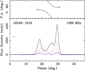
Figure 4: The polarization profile of PSR J1932+1059(=B1929+10) main pulse and J2048$-$1616 at 1369 MHz, observed by the author using Parkes telescope. The dashed line is the linear polarization intensity, and the circular polarization is plotted by the lower solid line. The polarization angle curve is plotted on the top of a profile.

Very special to the pulsars is the circular polarized emission, unique in the universe. Usually it is as strong as 10%, but in some pulsar components it could reach 70% mh04 . The circular polarization measurements have been comprehensively reviewed in hmxq98 ; yh06 . In summary, we found that circular polarization is not restricted to core components and, in some cases, reversals of circular polarization sense are observed across the conal emission. For core components, there is no significant correlation between the sense change of circular polarization and the sense of linear position-angle variation. These results are contradictory to the conclusions given by Radhakrishnan & Rankin rr90 based on early smaller sample of pulsar data. We found that in conal double profiles, the sense of circular polarization is correlated with the sense of position-angle variation. Pulsars with a high degree of linear polarization often have one hand of circular polarization across the whole profile. For most pulsars, the sign of circular polarization is same at 50 cm and 20 cm wavelengths, and the degree of polarization is similar, albeit with a wide scatter. Some pulsars are known to have frequency-dependent sign reversals. The diverse behavior of circular polarization may be generated in the emission process ggm01 or arise as a propagation effect ml04 .

3 Pulsars as probes for interstellar medium

The dispersion of the radio pulses is a very important tool, which can be used to not only identify radio emission from distant pulsars but also probe the ionized gas in the interstellar medium (ISM) which otherwise is difficult to detect and model. The scattering of radio signals measured from narrow radio pulses can be used to detect the randomness of electron distribution. The polarized radio signals of pulsars are Faraday rotated in the magnetized interstellar medium, so that pulsars act as key probes for the Galactic magnetic fields.

3.1 Electron density distribution in our Galaxy

The most knowledge of interstellar electron distribution comes from pulsar measurements. Using the observed dispersion measures of a sample of pulsars, $DM=\int_{\rm 0}^{\rm Dist}n_{e}dl$, one can get the electron density distribution if pulsar distances can be independently measured; or vice versa. The models for electron density distribution of our Galaxy have been constructed and constrained from the DMs and independent distance estimates of a large number of pulsars tc93 ; gbc01 ; cl02 ; cl03 , which consists of the thin electron disk, thick disk and spiral arms as well as bulge component. It is such an electron density model that can be used to estimate distances of most of pulsars from observed DMs so that we can know approximately how far a pulsar is located.

In fact, the interstellar medium is not smoothly distributed, but more or less random or irregularly clumpy, with only some large-scale preferred distribution in spiral arms and concentrated towards the Galactic plane. Note also that pulsars are point radio sources. They move very fast hllk05 . The interstellar medium randomly refracts and diffracts the pulsar signal and makes the pulsar scintillating and scattering. When pulsars are observed in many frequency channels for some time, one can see that pulsar signals scintillate both in time and observation channel frequency dimension – see excellent examples of so-called dynamic spectrum shown by Gupta et al. grl94 . The dynamic spectrum, which itself is the grey-plot of pulse intensity in the 2-D of observation frequency and time, shows the intensity correlation over both the time scale and frequency scale. Note that the randomness of the interstellar medium can be averaged over certain distance, so the distant pulsars do not scintillate much. The scintillation bandwidth is a function of frequency wmj+05 . High sensitivity observations can produce parabolic arcs in the secondary spectrum of the dynamic spectrum smc+01 , which depends on the velocity of scintillation pattern and geometry of the diffracting screen.

The more distant the pulsar is located, more the pulse signal is diffracted and scattered. This leads to the pulse broadening, especially at low frequencies. The most recent and largest data set for pulsar scattering have been obtained by Bhat et al bcc+04 , who observed 98 pulsars in several frequencies, from which, together with previous the pulse-broadening, $\tau$, is found to scale with observation frequency $\nu$ and DM, in the form of

$$\log\tau{\rm(ms)}\simeq-6.46+0.154\log(DM)+1.07\log(DM)^{2}-4.4\log(\nu/{\rm GHz}).$$ (3)

We considered the scattering effected on the polarized emission, and found that scattering can indeed flatten the PA curves lh04 . The simulations and the following observations by Camilo et al. crj+08 have confirmed such an effect.

3.2 Magnetic field structure of our Galaxy

For a pulsar at distance $D$ (in pc), the rotation measure (RM, in radians m^-2) is given by

$${\rm RM}=0.810\int_{0}^{D}n_{e}{\bf B}\cdot d{\bf l},$$ (4)

where $n_{e}$ is the electron density in cm^-3, ${\bf B}$ is the vector interstellar magnetic field in $\mu$G and $d{\bf l}$ is an elemental vector along the line of sight from a pulsar toward us (positive RMs correspond to fields directed toward us) in pc. With the $DM$ we obtain a direct estimate of the field strength weighted by the local free electron density

$$\langle B_{||}\rangle=\frac{\int_{0}^{D}n_{e}{\bf B}\cdot d{\bf l}}{\int_{0}^{D}n_{e}dl}=1.232\frac{RM}{DM},$$ (5)

where RM and DM are in their usual units of rad m^-2 and cm^-3 pc and $B_{||}$ is in $\mu$G. Previous analysis of pulsar RM data has often used the model-fitting method hq94 ; id99 , i.e., to model magnetic field structures in all of the paths from pulsars to us (observer), and fit the model to the observed RM data with the electron density model cl02 . Significant improvement can be obtained when both RM and DM data are available for many pulsars in a given region with similar lines of sight. Measuring the gradient of RM with distance or DM is the most powerful method of determining both the direction and magnitude of the large-scale field local in that particular region of the Galaxy hml+06 . One can get

$$\langle B_{||}\rangle_{d1-d0}=1.232\frac{\Delta{\rm RM}}{\Delta{\rm DM}},$$ (6)

where $\langle B_{||}\rangle_{d1-d0}$ is the mean line-of-sight field component in $\mu$G for the region between distances $d0$ and $d1$, $\Delta{\rm RM}={\rm RM}_{d1}-{\rm RM}_{d0}$ and $\Delta{\rm DM}={\rm DM}_{d1}-{\rm DM}_{d0}$. From all available data, we found that hml+06 magnetic fields in all inner spiral arms are counterclockwise when viewed from the North Galactic pole. On the other hand, at least in the local region and in the inner Galaxy in the fourth quadrant, there is good evidence that the fields in inter-arm regions are similarly coherent, but clockwise in orientation. There are at least two or three reversals in the inner Galaxy, probably occurring near the boundary of the spiral arms. The magnetic field in the Perseus arm cannot be determined well. The negative RMs for distant pulsars and extragalactic sources in fact suggest the inter-arm fields both between the Sagittarius and Perseus arms and beyond the Perseus arm are predominantly clockwise. See my recent reviews han08 ; han07 for more details and references therein.

4 Pulsar timing and gravitational waves

Pulsars emit pulses with accurate period ($P$). After time-of-arrival (TOA) of every pulse is measured (timing observations), one has to correct all measurements to the barycenter of the Solar system. It is easy to find that pulsars are slowing down due to radiation. The rate of period change ($\dot{P}$) can be measured. From $P$ and $\dot{P}$, one can estimate the magnetic field strength on the neutron star surface, $B=3.2\times 10^{19}\sqrt{P\dot{P}}$.

The timing data usually have some “noise”, not from measurement uncertainty but from the stars them-self. More interesting is that from timing data of young pulsars, there are spectacular changes in the rotation period, known as “glitch”. About 100 glitches have been observed from some 30 pulsars wmp+00 ; klg+03 ; zwm+08 . These glitches provide a penetrating means for investigation of pulsar interior structure.

Millisecond pulsars are very stable (small $\dot{P}$) and have very tiny timing-noise. By timing millisecond pulsars, especially pulsars in binary system provide tools to study gravitational theory. The orbital motion of pulsars and relativistic effects can be easily measured through the pulse time delay. The first extra Solar planet was discovered by using timing the millisecond pulsar PSR B1257+12 wf92 . The gravitational redshift and time dilation as well as the Shapiro delay have been detected from a number of pulsar binary system s04 , and the masses of pulsars as well as their companions can be measured very accurately.

The most exciting is the discovery of a relativistic binary pulsar, PSR B1913+16 ht75 which have been used for examination of the general relativity. The orbital shrink, because of the gravitational wave radiation, has been detected from this pulsar – which reveals a new radiation form in the nature and was awarded the Nobel Prize in 1993. The newly discovered binary pulsar lbk+04 can act as the testbed even better ksm+06 .

References

- (1) A. Hewish, S.J. Bell, J.D. Pilkington et al: Nature 217, 709 (1968)
- (2) T. Gold: Nature 218, 731 (1968)
- (3) F. Pacini: Nature 219, 145 (1968)
- (4) V.M. Kaspi: Advances in Space Sciences 21, 167 (1998)
- (5) G. Hobbs, D.R. Lorimer, A.G. Lyne, M. Kramer: MNRAS 360, 974 (2005)
- (6) C. Wang, D. Lai, J.L. Han: ApJ 639, 1007 (2006)
- (7) X.H. Sun, J.L. Han: MNRAS 350, 232 (2004)
- (8) D.M. Gould, A.G. Lyne: MNRAS 301, 235 (1998)
- (9) M.C. Allen, D.B. Melrose: Proc. Astron. Soc. Australia, 4, 365 (1982)
- (10) J.J. Barnard, J. Arons: ApJ 302, 138
- (11) N.D.R. Bhat, J.M. Cordes, F. Camilo, et al: ApJ 605, 759
- (12) M. Blaskiewicz, J.M. Cordes, I. Wasserman: ApJ 370, 643 (1991)
- (13) F. Camilo, J. Reynolds, S. Johnston et al: ApJ, in press=arXiv:0802.0494 (2008)
- (14) J.M. Cordes, T.J.W. Lazio: astro-ph/0207156v3 (2002)
- (15) J.M. Cordes, T.J.W. Lazio: astro-ph/0301598v1 (2003)
- (16) J.M. Cordes, P.C.C. Freire, D. Lorimer, et al: ApJ 637, 446 (2006)
- (17) J.M. Cordes, J.M. Rankin, D.C. Backer: ApJ 223, 961 (1978)
- (18) A.A. Deshpande, J.M. Rankin: ApJ 524, 1008 (1999)
- (19) A.A. Deshpande, J.M. Rankin: MNRAS 322, 438 (2001)
- (20) P.C. Freire, Y. Gupta, S.M. Ransom, C.H. Ishwara-Chandra: ApJ 606, 53 (2004)
- (21) R.T. Gangadhara: A&A 327, 155 (1997)
- (22) R.T. Gangadhara: ApJ 609, 335 (2004)
- (23) R.T. Gangadhara: ApJ 628, 923 (2005)
- (24) R.T. Gangadhara, Y. Gupta: ApJ 555, 31 (2001)
- (25) M. Gedalin, P E. Gruman, D. B. Melrose: MNRAS 325, 715 (2001)
- (26) J.A. Gil, A.G. Lyne, J.M. Rankin et al: A&A 255, 181 (1992)
- (27) G.C. Gómz, R.A. Benjamin, D.P. Cox: ApJ 122, 908 (2001)
- (28) Y. Gupta, B.J. Rickett, A.G. Lyne: MNRAS 269, 1035 (1994)
- (29) J.L. Han: IAU Symp. 242, 55 (2007)
- (30) J.L. Han: Nuclear Physics B Proc. Supp. 175, 62 (2008)
- (31) J.L. Han, R.N. Manchester: MNRAS 320, L35 (2001)
- (32) J.L. Han, R.N. Manchester, R.X. Xu, G.J. Qiao: MNRAS 300, 373 (1998)
- (33) J.L. Han, R.N. Manchester, A.G. Lyne et al: ApJ 642, 868 (2006)
- (34) J.L. Han, G.J. Qiao: A&A, 288, 759 (1994)
- (35) R.A. Hulse, J.H. Taylor: ApJ 201, 55 (1975)
- (36) C. Indrani, A.A. Deshpande: New Astronomy, 4, 33 (1999)
- (37) B.C. Joshi, M.A. Malaughlin, M. Kramer et al.: arXiv 0710.2955 (2007)
- (38) M. Kramer, I.H. Stairs, R.N. Manchester et al: Science 314, 97 (2006)
- (39) A. Krawczyk, A.G. Lyne, J.A. Gil et al: MNRAS 340, 1087 (2003)
- (40) X.H. Li, J.L. Han: A&A 410, 253 (2003)
- (41) J.R. Lin, S.N. Zhang: ApJ 615, 133 (2004)
- (42) D. Lorimer, M. Kramer: Handbook of Pulsar Astronomy, Cambridge University Press (2005)
- (43) A.G. Lyne, M. Burgay, M. Kramer et al: Sciences 303, 1153 (2004)
- (44) A.G. Lyne, R.N. Manchester: MNRAS 234, 477 (1988)
- (45) A.G. Lyne, F. Graham-Smith: Pulsar Astronomy, Cambridge University Press (2006)
- (46) R.N. Manchester: PASA 2, 334 (1975)
- (47) R.N. Manchester: JApA 16, 107 (1995)
- (48) R.N. Manchester, J.L. Han: ApJ 609, 354 (2004)
- (49) R.N. Manchester, J.L. Han, G.J. Qiao: MNRAS 295, 280 (1998)
- (50) R.N. Manchester, G.B. Hobbs, A. Teoh, M. Hobbs: AJ 129, 1993 (2005)
- (51) R.N. Manchester, A.G. Lyne, F. Camilo, et al: MNRAS 328, 17 (2001)
- (52) O. Maron, J. Kijak, M. Kramer, R. Wielebinski: A&AS 147, 195 (2000)
- (53) D. Melrose, Q.Lou: MNRAS 352, 915 (2004)
- (54) D. Melrose, A. Miller, A. Karastergiou, Q. Lou: MNRAS 365, 638 (2006)
- (55) D. Page, S. Reddy: ARNPS 56, 327 (2006)
- (56) S.A. Petrova: A&A 378, 883 (2001)
- (57) V. Radhakrishnan, D.J. Cooke: ApL 3, 225 (1969)
- (58) V. Radhakrishnan, J.M. Rankin: ApJ 352, 258 (1990)
- (59) J.M. Rankin: ApJ 274, 333 (1983)
- (60) J.M. Rankin: ApJ 352, 247 (1990)
- (61) J.M. Rankin: ApJS 85, 145 (1993)
- (62) J.M. Rankin: ApJ 405, 285 (1993)
- (63) P. Slane, AIP conf.proc. Vol. 968, 143 (2008)
- (64) I.H. Stairs, Sciences 304, 547 (2004)
- (65) I.H. Stairs, A.G. Lyne, S.L. Shemar: Nature 406, 484 (2000)
- (66) D.R. Stinebring, J.M. Cordes, J.M. Rankin et al: ApJS 55, 247 (1984a)
- (67) D.R. Stinebring, J.M. Cordes, J.M. Weisberg et al: ApJS 55, 279 (1984b)
- (68) D.R. Stinebring, M.A. McLaughlin, J.M. Cordes, et al: ApJ 549, 97 (2001)
- (69) J.H. Taylor, J.M. Cordes: ApJ 411, 674 (1993)
- (70) S.E. Thorsett: ApL 377, 263 (1991)
- (71) N. Wang, R.N. Manchester, S.Johnston et al.: MNRAS 358, 270 (2005)
- (72) N. Wang, R.N. Manchester, S.Johnston: MNRAS 377, 1383 (2007)
- (73) N. Wang, R.N. Manchester, R.T. Pace et al.: MNRAS 317, 843 (2000)
- (74) J.M. Weisberg, J.M. Cordes, S.C. Lundgren et al: ApJS 121, 171 (1999)
- (75) J.M. Weisberg, J.H. Taylor: ApJ 576, 942 (2002)
- (76) A. Wolszczan, D.A. Frail: Nature 355, 145 (1992)
- (77) X.J. Wu, X. Gao, J.M. Rankin, W. Xu, V.M. Malofeev: AJ 116, 1984 (1998)
- (78) X.J. Wu, R.N. Manchester, A.G. Lyne, G.J. Qiao: MNRAS 261, 630 (1993)
- (79) R.X. Xu, G.J. Qiao, J.L. Han: A&A 323, 395 (1997)
- (80) X.P. You, J.L. Han: ChJAA 6, 237 (2006)
- (81) Y.L. Yue, R.X. Xu, W.W. Zhu: Advance in Space Science 40, 1491 (2007)
- (82) W.Z. Zou, N. Wang, R.N. Manchester, et al: MNRAS 384, 1063 (2008)