Maximal Information Transfer and Behavior Diversity in Random Threshold Networks

Abstract

Random Threshold Networks (RTNs) are an idealized model of di- luted, non-symmetric spin glasses, neural networks or gene regulatory networks. RTNs also serve as an interesting general example of any coordinated causal system. Here we study the conditions for maximal information transfer and behavior diversity in RTNs. These conditions are likely to play a major role in physical and biological systems, per- haps serving as important selective traits in biological systems. We show that the pairwise mutual information is maximized in dynami- cally critical networks. Also, we show that the correlated behavior di- versity is maximized for slightly chaotic networks, close to the critical region. Importantly, critical networks maximize coordinated, diverse dynamical behavior across the network and across time: the informa- tion transmission between source and receiver nodes and the diversity of dynamical behaviors, when measured with a time delay between the source and receiver, are maximized for critical networks.

Institute for Biocomplexity and Informatics

University of Calgary

2500 University Drive NW, Calgary

Alberta, T2N 1N4, Canada

1 Introduction

The random Boolean networks (RBNs) model was initially introduced as an idealized model of genetic regulatory networks [1]. Since then, the RBN model has attracted much interest in a wide variety of fields, ranging from cell differentiation and evolution to social and physical spin systems. The dynamics of RBNs can be classified as ordered, chaotic, or critical, as a function of the average in-degree $k$ and the bias $p$ in the choice of Boolean functions [2]. The central issue of the research on the RBN model is the characterization of the critical transition between ordered and chaotic phases [3]. These two regimes produce very different emergent dynamical behaviors. Networks operating in the ordered regime are intrinsically robust, but exhibit simple dynamics. This robustness is reflected in the dynamical stability of the network both under structural perturbations and transient perturbations. In contrast, networks in the chaotic regime are extremely sensitive to small perturbations, which rapidly propagate throughout the entire system. The phase transition between the ordered and chaotic regimes represents a tradeoff between stability and access to a wide range of dynamic behavior to respond to a variable environment.

Recently it has been shown that the pairwise mutual information exhibits a jump discontinuity at the critical values of $k$ and $p$ [4]. Here, we extend these results to a second class of discrete dynamical networks called Random Threshold Networks (RTN), which were first studied as diluted, non-symmetric spin glasses, neural networks and gene regulatory networks [5-9]. More specifically, we study the conditions for maximal information transfer and behavior diversity in RTNs. We show that the pairwise mutual information is maximized in critical networks. Also, we show that the correlated behavior diversity is maximized for slightly chaotic networks, close to the critical region when measured with no delay between source and receiver nodes. In contrast, when the delay between the measurement of source and receiver nodes is increased, correlated behavior complexity and diversity is maximized for critical networks. These results support the hypotheses that critical networks provide an optimal information transfer between the elements of the network, and optimal coordination of diverse behavior when there is a time delay between source and receiver nodes, while slightly chaotic networks have an optimal capacity for coordinating most diverse dynamical behavior in the absence of such a delay.

2 RTN model

The RTN model consists of $N$ randomly interconnected binary variables (spins) with states $\sigma_{i}\in\{\pm 1\}$, $i=0,...,N-1$ [9]. Each variable has associated a function:

$$\varphi_{i}(t)=\sum_{j=0}^{N-1}\omega_{ij}\sigma_{j}(t)+\theta,$$ (1)

where the interaction weights take discrete values $\omega_{ij}\in\{\pm 1\}$ with equal probability, and the discrete threshold $\theta$ is fixed. Without loosing generality, in the following discussion the threshold parameter is set to $\theta=0$. If node $i$ does not receive signals from node $j$, one has $\omega_{ij}=0$. The average number $k$ of non-zero interaction weights represents the average connectivity (in-degree) of the nodes in the network. The variable $\sigma_{i}$ will change its state at each time step according to the rule:

$$\sigma_{i}(t+1)=sign(\varphi_{i}(t)).$$ (2)

where $sign(x)=1$ if $x\geq 0$ and $sign(x)=-1$ if $x<0$.

3 Information transfer and behavior diversity

The average pairwise correlation has been used to characterize the typical dynamics of pairs of nodes [9]. The average correlation between two nodes $i$ and $j$ is defined as:

$$C_{ij}=\left|\frac{1}{T}\sum_{t=0}^{T-1}\sigma_{i}(t)\sigma_{j}(t)\right|,$$ (3)

where $T$ is the length of the time series over which the correlation is measured. If the dynamical activity of two nodes $i$ and $j$ is (anti-)correlated, i.e. if $\sigma_{i}(t)$ and $\sigma_{j}(t)$ always have either the same or the opposite sign, one has $C_{ij}=1$. If the relationship between the signs of $\sigma_{i}(t)$ and $\sigma_{j}(t)$ occasionally changes then $0\leq C_{ij}<1$. It has been shown that the quantity:

$$\left\langle C\right\rangle=N^{-2}\left\langle C_{ij}\right\rangle,$$ (4)

(averaged over the RTN ensemble) exhibits a second order phase transition at a critical average connectivity $k_{c}=2$ [9]. For $k<k_{c}$, the nodes are typically frozen, with $\left\langle C_{ij}\right\rangle\simeq 1$. For $k\geq k_{c}$, in the limit of large $N$, $\left\langle C_{ij}\right\rangle$ undergoes a transition at $k_{c}$, vanishing for larger $k>>k_{c}$ [9].

Now, let us define the average activity $A_{i}$ of a node $i$ as following:

$$A_{i}=1-\left|\frac{1}{T}\sum_{t=0}^{T-1}\sigma_{i}(t)\right|,$$ (5)

Frozen nodes, which do not change their states have an activity $A_{i}=0$, while the nodes who occasionally change their state have an activity $0<A_{i}\leq 1$. The average activity

$$\left\langle A\right\rangle=N^{-1}\left\langle A_{i}\right\rangle$$ (6)

is largest $\left\langle A\right\rangle\sim 1$ in the chaotic phase $k>k_{c}$, and by decreasing $k$ undergoes a second order phase transition at $k_{c}$, vanishing for $k=0$.

We can define the entropy [10] of the node $i$, $i=0,1,...,N-1$, as:

$$H_{i}=-\sum_{\alpha\in\{\pm 1\}}p_{\alpha}(\sigma_{i}(t))\log_{2}p_{\alpha}(\sigma_{i}(t)),$$ (7)

where $p_{\alpha}(\sigma_{i}(t))$ is the probability of the symbol $\alpha\in\{\pm 1\}$ in the time series $\{\sigma_{i}(t)\}$, $i=0,1,...,N-1$. The average entropy of the RTN ensemble is:

$$\left\langle H\right\rangle=N^{-1}\left\langle\sum_{i}H_{i}\right\rangle.$$ (8)

Both, the activity $A$ and the entropy $H$ measure the diversity of the dynamics of the nodes in the RTN ensemble as a function of their connectivity $k$.

The mutual information [11] between the nodes $i$ and $j$ as a function of the time lag $\tau=0,1,2,...$ is defined as following:

$$I_{ij}(\tau)=\sum_{\alpha\in\{\pm 1\}}\sum_{\beta\in\{\pm 1\}}p_{\alpha\beta}(\sigma_{i}(t),\sigma_{j}(t+\tau))\log_{2}\left(\frac{p_{\alpha\beta}(\sigma_{i}(t),\sigma_{j}(t+\tau))}{p_{\alpha}(\sigma_{i}(t))p_{\beta}(\sigma_{j}(t))}\right).$$ (9)

Here, $p_{\alpha}(\sigma_{i}(t))$ and $p_{\beta}(\sigma_{i}(t+\tau))$ are the probabilities of the symbols $\alpha,\beta\in\{\pm 1\}$ in $\{\sigma_{i}(t)\}$ and respectively $\{\sigma_{j}(t)\}$, and $p_{\alpha\beta}(\sigma_{i}(t),\sigma_{j}(t+\tau))$ is the probability of the pair $(\alpha,\beta)$ in $\{(\sigma_{i}(t),\sigma_{j}(t+\tau))\}$. $I_{ij}(\tau)$ measures the extent to which information about node $i$ at time $t$ influences node $j$ at time $t+\tau$. The propagation of information may be indirect, i.e. both nodes are influenced by a common node through previous time steps. The above probabilities can be easily estimated as following:

$$p_{\alpha\beta}(\sigma_{i}(t),\sigma_{j}(t+\tau))=\frac{\sum_{t=0}^{T-\tau}\delta(\sigma_{i}(t);\alpha)\delta(\sigma_{j}(t+\tau);\beta)}{\sum_{\alpha\in\{\pm 1\}}\sum_{\beta\in\{\pm 1\}}\sum_{t=0}^{T-\tau}\delta(\sigma_{i}(t);\alpha)\delta(\sigma_{j}(t+\tau);\beta)},$$ (10)

$$p_{\alpha}(\sigma_{i}(t))=\sum_{\beta\in\{\pm 1\}}p_{\alpha\beta}(\sigma_{i}(t),\sigma_{j}(t+\tau)),$$ (11)

$$p_{\beta}(\sigma_{i}(t))=\sum_{\alpha\in\{\pm 1\}}p_{\alpha\beta}(\sigma_{i}(t),\sigma_{j}(t+\tau)),$$ (12)

where

$$\delta(x;y)=\left\{\begin{array}[]{lll}1&if&x=y\\ 0&if&x\neq y\end{array}\right.,$$ (13)

is the Dirac delta function, and $T$ is the length of the considered time series. In order to characterize the information propagation through the entire network, we define the average pairwise mutual information for the RTN ensemble as following:

$$\left\langle I(\tau)\right\rangle=N^{-2}\left\langle\sum_{i,j}I_{ij}(\tau)\right\rangle.$$ (14)

Because the number of pairs $(i,j)$ that contribute significantly to the sum is expected to be at most of order $N$, it is convenient to work with the quantity

$$I_{N}(\tau)=N\left\langle I(\tau)\right\rangle,$$ (15)

which approaches a nonzero constant in the large-$N$ limit [4].

One can define the pairwise correlated behavior in several ways:

1. as the product between the activity of the nodes and their correlation:

   $$D_{ij}=\frac{1}{2}(A_{i}+A_{j})C_{ij},$$ (16)

   with the ensemble average given by:

   $$\left\langle D\right\rangle=N^{-2}\left\langle D_{ij}\right\rangle.$$ (17)

2. as a product between the entropy of the nodes and their correlation:

   $$F_{ij}=\frac{1}{2}(H_{i}+H_{j})C_{ij},$$ (18)

   with the ensemble average given by:

   $$\left\langle F\right\rangle=N^{-2}\left\langle F_{ij}\right\rangle.$$ (19)

3. as the product between the entropy of the nodes and their mutual information:

   $$Q_{ij}(\tau)=\frac{1}{2}(H_{i}+H_{j})I_{ij}(\tau),$$ (20)

   with the ensemble average given by:

   $$Q_{N}(\tau)=\frac{1}{2}N^{-1}\left\langle(H_{i}+H_{j})I_{ij}(\tau)\right\rangle.$$ (21)

Obviously, these quantities measure the correlated behavior diversity. For example, $D_{ij}$ and $F_{ij}$ are high only if both the activity (entropy) of the nodes and their correlation are simultaneously high. This means both that the nodes are changing, and that they are changing in a correlated fashion. Also, assuming that mutual information is a correlation measure, we may say that $Q_{ij}(\tau)$ measures the diversity of correlated dynamical behavior between the present $t$ and the future at $t+\tau$. Thus, by locating the ensemble of networks with a connectivity $k$ which maximizes these measures, we have found the dynamical region which exhibits the most correlated behavior diversity in the present (for $D$, $F$), and between the present and the future (for $Q(\tau)$).

4 Numerical results

Since the above defined quantities are not yet analytically accessible, numerical simulations are necessary for their estimation. The simulation procedure is similar to the one described in [3, 4]. For networks of size $N=10^{3}$, we simulated the dynamics for $10^{3}$ steps to eliminate the transient dynamics, and collected a time series of length $T=10^{4}$. Also, we averaged over $10^{3}$ distinct, randomly generated networks with $100$ runs from different randomly chosen initial states for each network. We should note that the ensemble averages are computed using a Monte Carlo procedure which includes data from all the attractors generated in the calculation. For example, in order to calculate $\left\langle C\right\rangle$ we sample $C_{i,j}$ randomly over $S=10^{3}$ networks and $R=100$ runs from different initial states, and we discard the transient dynamics for each run. The sampling is done by computing $C_{i,j}$ for $M=100N$ randomly generated pairs $m\equiv random(i,j)$, in each run. All the obtained samples $C_{m}$ are then used to calculate an approximation of the ensemble average as:

$$\left\langle C\right\rangle\simeq\frac{1}{SRM}\sum_{s=1}^{S}\sum_{r=1}^{R}\sum_{m=1}^{M}C_{m}.$$ (22)

In Figure 1 we give the average activity $\left\langle A\right\rangle$, the average correlation $\left\langle C\right\rangle$, the entropy $\left\langle H\right\rangle$ and their numerical derivatives with respect to $k$: $d\left\langle A\right\rangle/dk$, $\left|d\left\langle C\right\rangle/dk\right|$, $d\left\langle H\right\rangle/dk$. One can see that all three quantities exhibit a phase transition around $k_{c}^{\prime}\simeq 2.2$. The deviation from the large-network-size limit value of $k_{c}=2$, when $N\rightarrow\infty$, is due to the finite size of the simulated networks: $\Delta k_{c}=k_{c}^{\prime}-k_{c}\simeq 0.2$.

The average correlated behavior defined by $\left\langle D\right\rangle$ and $\left\langle F\right\rangle$ is shown in Figure 2. Both $\left\langle D\right\rangle$ and $\left\langle F\right\rangle$ reach their maximum value in the slightly chaotic regime, around $k_{DF}^{\prime}\simeq 2.6$ ($k_{DF}\simeq 2.4$, corrected for the finite size effect, as noted above).

In Figure 3 we show the average mutual information $I_{N}(\tau)$ as a function of the time lag $\tau=0,1,...,40$. The mutual information also has a maximum value around the critical value $k_{c}^{\prime}\simeq 2.2$ ($k_{c}\simeq 2.0$, corrected for the finite size effect). It is interesting to note that $I_{N}(\tau)$ decreases with $\tau$, having a maximum value for $\tau=0$. This shows that information gained about the state of one node given the state of another node decays over time, as one might expect. In addition, the numerical simulation suggests that $I_{N}(\tau)$ is localizing around the critical value $k_{c}$ when the time lag $\tau$ increases, converging to a delta function for large $\tau$: $I_{N}(\tau)\rightarrow\delta(k,k_{c})$.

The average correlated behavior $Q_{N}(\tau)$ is given in Figure 4. The maximum of $Q_{N}(\tau)$ shifts to the left when $\tau$ increases, from $k_{c}^{\prime}\simeq 2.4$ when $\tau=0$, to $k_{c}\simeq 2.2$ when $\tau=40$, and it seems to converge to $k_{c}$ for large $\tau$.

5 Discussion and conclusion

Shannon information measures the information transmission down a noisy channel with a decoder of indefinite computational power and seeks to maximize information transmission [10]. Cells, other biological and other physical systems, do not have decoders of arbitrary power. More, it seems plausible that in cells, neural systems, and other tissues, natural selection will have acted to maximize both information transfer across the network, and the diversity of complex behaviors that can be coordinated within a causal network. We have shown that the pairwise mutual information is maximized in critical RTNs. Also, we have shown that the diversity of complex correlated behavior is maximized for slightly chaotic RTNs, close to the critical region using two measures of correlated diversity, $D$ and $F$, with no temporal delay between signaling and receiving nodes. Importantly, in the presence of a delay, $\tau$, between signaling and receiving nodes, maximum diversity of complex coordinated behaviors clearly shifts towards critical networks as the delay increases. Ordered networks have convergent trajectories, and hence ”forget” their past; chaotic networks show sensitivity to initial conditions, and thus they, too, forget their past and are unable to act reliably. Critical networks, with trajectories that, on average, neither diverge or converge, seem best able to bind past to future. In short, our results show that in the presence of a delay, hence time binding, critical networks maximize information transfer between source and receiver nodes, i.e. they maximize pairwise mutual information, and simulataneously maximize the diversity and complexity of behaviors that can be correlated by that information transfer.

Given the potential biological implications, it is of interest that recent data suggest that genetic regulatory networks in eukaryotic cells are dynamically critical [12-14]. Also, recent experiments conducted on rat brain slices show that these neural tissues are critical [15]. RTN are simple Boolean models of threshold neural networks. Further work with random Boolean networks, RBN, will attempt to extend these results to this class of disordered causal systems, and will extend these results to communication between networks. We note that recent results have shown that critical RBN maximize power efficiency [3, 16]. Maximum energy efficiency occurs if work cycles are performed infinitely slowly. Cells must do work cycles to reproduce. Infinitely slow cell reproduction would fail in the Darwinian race. Maximum power efficiency occurs at a finite, defined, displacement from equilibrium. Our hope is that subsequent work will establish that cells and tissues, as evolved, far from equilibrium evolved systems, simultaneously maximize information transfer, the complexity and diversity of dynamical behaviors that can be coordinated, and the power efficiency with which these complex diverse behaviors are carried out. Such results may help formulate a far from equilibrium theory for living systems.

Using random threshold boolean nets as simple models of complex causal systems we have studied information transfer between source and receiver nodes. We have shown that critical RTN maximize both information transfer, and the complexity and diversity of dynamical behaviors that can be coordinated across the network and time.

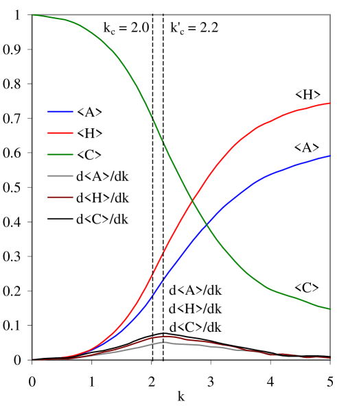
Figure 1: The average activity $\left\langle A\right\rangle$, the average correlation $\left\langle C\right\rangle$, the entropy $\left\langle H\right\rangle$ and their numerical derivatives with respect to $k$: $d\left\langle A\right\rangle/dk$, $d\left\langle C\right\rangle/dk$, $d\left\langle H\right\rangle/dk$.

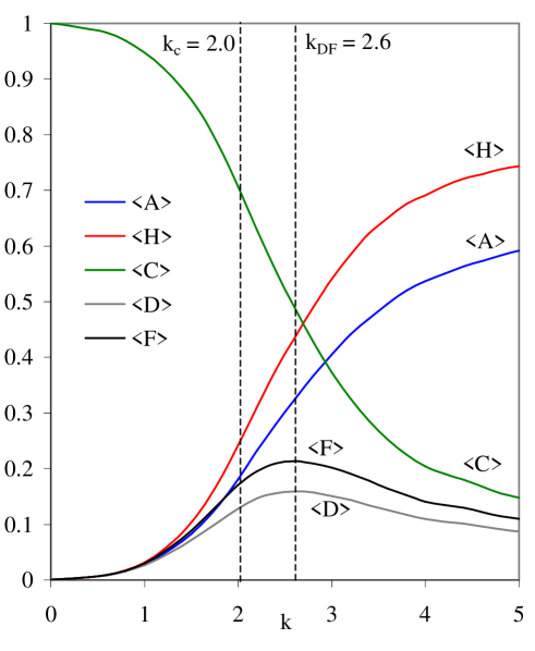
Figure 2: The average activity $\left\langle A\right\rangle$, the average correlation $\left\langle C\right\rangle$, the entropy $\left\langle H\right\rangle$ and the average correlated behavior defined by $\left\langle D\right\rangle$ and $\left\langle F\right\rangle$.

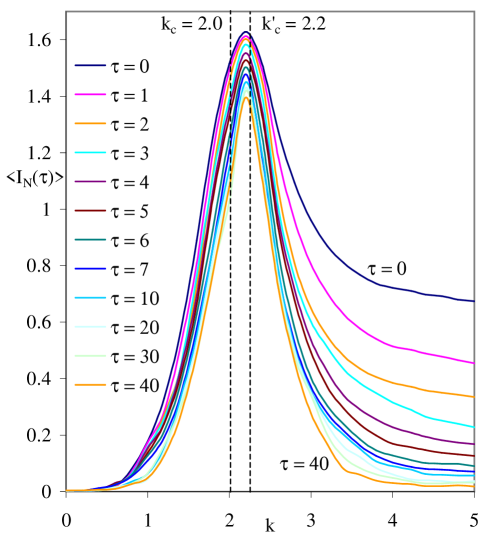
Figure 3: The average mutual information $I_{N}(\tau)$ as a function of the time lag $\tau=0,1,...,7$.

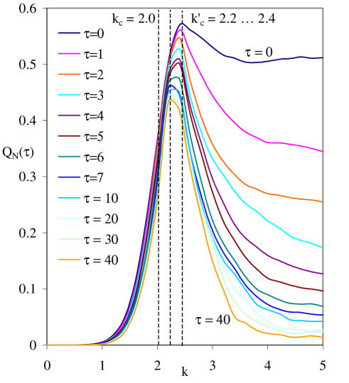
Figure 4: The average correlated behavior $Q_{N}(\tau)$ as a function of the time lag $\tau=0,1,...,7$.

References

- [1] S. A. Kauffman, The Origins of Order: Self-Organization and Selection in Evolution (Oxford University Press, New York, 1993).
- [2] M. Aldana, S. Coopersmith, L. P. Kadanoff, Boolean dynamics with random couplings, in Perspectives and Problems in Nonlinear Science. Springer Applied Mathematical Sciences Series. Ehud Kaplan, Jerrold E. Marsden, and Katepalli R. Sreenivasan Eds., 23-89 (Springer, New-York, 2003).
- [3] M. Andrecut, S. A. Kauffman, Energy and criticality in random Boolean networks, Phys. Lett. A, 372(27-28), 4757-4760 (2008).
- [4] A. S. Ribeiro, S. A. Kauffman, J. Lloyd-Price, B. Samuelsson, J. E. S. Socolar, Mutual information in random Boolean models of regulatory networks, Phys. Rev. E 77, 011901 (2008).
- [5] B. Derrida, E. Gardner, A. Zippelius, An exactly solvable asymmetric neural network model, Europhys. Lett. 4, 167 (1987).
- [6] K. Kürten, Critical phenomena in model neural networks, Phys. Lett. A 129, 156-160 (1988).
- [7] S. Bornholdt, T. Röhl, Self-organized critical neural networks, Phys. Rev. E 67, 066118 (2003).
- [8] T. Rohlf, S. Bornholdt, Criticality in random threshold networks: Annealed approximation and beyond, Physica A 310, 245-259 (2002)
- [9] T. Rohlf, S. Bornholdt, Self-organized criticality and adaptation in discrete dynamical networks (arXiv:0811.0980, 2008).
- [10] T.M. Cover, J.A. Thomas, Elements of Information Theory (Wiley, New York, 1991).
- [11] M. Andrecut, S. A. Kauffman, A simple method for reverse engineering causal networks, J. Phys. A: Math. Theor. 39, L647 (2006).
- [12] R. Serra, M. Villani, and A. Semeria, Genetic networks models and statistical properties of gene extression data in knock-out experiments, J. Theor. Biol. 227, 149-157 (2004).
- [13] I. Shmulevich, S. A. Kauffman, and M. Aldana, Eukaryotic cells are dynamically ordered or critical but not chaotic, Proc. Natl. Acad. Sci. U.S.A. 102, 13439 (2005).
- [14] P. R m , J. Kesseli, and O. Yli-Harja, Perturbation avalanches and criticality in gene regulatory networks, J. Theor. Biol. 242, 164 (2006).
- [15] D. Hsu, J. M. Beggs, Neuronal avalanches and criticality: A dynamical model for homeostasis, Neurocomputing 69, 1134-1136 (2006).
- [16] H. A. Carteret, K. J. Rose, S. A. Kauffman, Maximum power efficiency and criticality in random Boolean networks, Phys. Rev. Lett. 101, 218702 (2008).