Degrees of Freedom of a Communication Channel: Using Generalised Singular Values

Abstract

A fundamental problem in any communication system is: given a communication channel between a transmitter and a receiver, how many “independent” signals can be exchanged between them? Arbitrary communication channels that can be described by linear compact channel operators mapping between normed spaces are examined in this paper. The (well-known) notions of degrees of freedom at level $\epsilon$ and essential dimension of such channels are developed in this general setting. We argue that the degrees of freedom at level $\epsilon$ and the essential dimension fundamentally limit the number of independent signals that can be exchanged between the transmitter and the receiver. We also generalise the concept of singular values of compact operators to be applicable to compact operators defined on arbitrary normed spaces which do not necessarily carry a Hilbert space structure. We show how these generalised singular values can be used to calculate the degrees of freedom at level $\epsilon$ and the essential dimension of compact operators that describe communication channels. We describe physically realistic channels that require such general channel models.

I Introduction

The basic consideration in this paper can be stated as follows: given an arbitrary communication channel, is it possible to evaluate the number of independent sub-channels or modes available for communication. Though this question is not generally examined explicitly, it plays an important role in various information theoretic problems.

A rigorous proof of Shannon’s famous capacity result [1] for continuous-time band-limited white Gaussian noise channels requires a calculation of the number of approximately time-limited and band-limited sub-channels (see e.g. [2, ch. 8] and [3, 4]). This result can be generalised to dispersive/non-white Gaussian channels using the water-filling formula [1, 2]. In order to use this formula, one needs to diagonalise the channel operator and allocate power to the different sub-channels or modes based on the singular values of the corresponding sub-channel. One therefore needs to calculate the modes and the power transferred (square of the singular values) on each one of these sub-channels to calculate the channel capacity.

The water-filling formula has been used extensively in order to calculate the capacity of channels that use different forms of diversity. In particular, the capacity of multiple-input multiple-output (MIMO) antenna systems has been calculated using this water-filling formula for various conditions imposed on the transmitting and the receiving antennas (see e.g. [5] and references therein). Water-filling type formulas have been used for other multi-access schemes such as OFDM-MIMO [6] and CDMA [7] (see also Tulino [8, sec 1.2] and references therein). More recently, several papers have examined the number of degrees of freedom available in spatial channels [9, 10, 11, 12, 13]. Questions of this nature have also been studied in other contexts such as optics [14] and spatial sampling of electromagnetic waves [15, 16].

Both types of results, the modes of communication used for the water-filling formula and the number of degrees of freedom of spatial channels use the singular value decomposition (SVD) theorem. One can use SVD to diagonalise the channel operator and the magnitude of the singular values determines the power transferred on each of the sub-channels. The magnitude of these singular values can therefore be used to calculate the number of degrees of freedom of the channel (see e.g. [12, 9]). However, the SVD theorem is only applicable to compact operators defined on Hilbert spaces. An implicit and valid assumption that is used in these papers is that the operators describing the communication channels are defined on Hilbert spaces. These results can therefore not be generalised directly to communication systems that are modeled by operators defined on normed spaces that do not admit an inner product structure. There are several instances of practical channels that can not be modeled using operators defined on inner-product spaces (see Section II-A for examples). In this paper, we develop a general theory that enables one to evaluate the number of degrees of freedom of such systems.

We wish to examine if it is possible to evaluate the number of parallel sub-channels available in general communication systems that can be described using linear compact operators. Any communication channel is subject to various physical constraints such as noise at the receiver or finite power available for transmission. If the channel can be modeled via a linear compact operator, then these constraints ensure that only finitely many independent channels are available for communication. Roughly speaking, we call the number of such channels the number of degrees of freedom of the communication system (see Section III for a precise definition). Note that if the channel is modeled using a linear operator that is not compact then it will in fact have infinitely many parallel sub-channels, or some channels that can transfer an infinite amount of power (see Theorem III.10 below and the discussion following it). It could hence be argued that the theory presented in this paper is the most general theory needed to model physically realistic channels.

We give novel definitions for the terms degrees of freedom and essential dimension in the following section. Even though these terms have been used interchangeably in the literature, we distinguish between the two. The essential dimension of a channel is useful for channels that have numbers of degrees of freedom that are essentially independent of the receiver noise level (e.g. the time-width/band-width limited channels in Slepian’s work [17]). Also, we generalise the notion of singular values to compact operators defined on normed spaces and explain how these generalised singular values can be used to compute degrees of freedom and the essential dimension.

I-A Channel Model

We assume that a communication channel between a transmitter and a receiver can be modeled as follows. Let $X$ be a linear vector space of functions that the transmitter can generate and let $Y$ be a linear vector space of functions that the receiver can measure. We assume the existence of a linear operator $T:X\rightarrow Y$ that maps each signal generated by a transmitter to a signal that a receiver can measure. We also assume that there is a norm $\|\cdot\|_{X}$ on $X$ and a norm $\|\cdot\|_{Y}$ on $Y$. This model is very general and can be applied to various situations of practical relevance.

For instance, consider a MIMO communication system wherein the transmitter symbol waveform shape on each antenna is a raised cosine. In this case we can think of the space of transmitter functions $X$ to be (more precisely, to be parametrised by) the $n$-dimensional complex space $\mathbb{C}^{n}$ that determines the phase and amplitude of the raised cosine waveform on each antenna. Here $n$ is the number of transmitting antennas. Also, we can think of the space of receiver functions as $\mathbb{C}^{m}$, where $m$ is the number of receiving antennas. $T$ in this context is a channel matrix, representing the linearized channel operator that depends on the scatterers in the environment.

Alternatively, consider a MIMO communication system in which the transmitter symbols are not fixed but can be any waveform of time. Suppose the symbol time is fixed to $t_{s}$ seconds. In this case, we can think of the space of transmitter functions, $X$, as the space $\mathcal{L}^{2}([0,t_{s}],\mathbb{C}^{n})$ of $\mathbb{C}^{n}$-valued square integrable functions defined on $[0,t_{s}]$. Similarly, we can think of the space of receiver functions, $Y$, as the space $\mathcal{L}^{2}([0,t_{s}],\mathbb{C}^{m})$. Again, $T$ is the channel operator.

Irrespective of the precise form of the underlying spaces $X$ and $Y$, we always call elements of $X$ transmitter functions and the elements of $Y$ receiver functions. Also, we call the space $X$ the space of transmitter functions and the space $Y$ the space of receiver functions. In particular, we do not distinguish between the two different physical situations: a) the elements of $X$ are functions of time and b) the elements of $X$ are vectors in some finite dimensional space. This should cause no confusion and we use this convention for the remainder of this document.

We now restrict ourselves to situations where there is a source constraint $\|\cdot\|_{X}\leq P$ that can be imposed on the space of transmitter functions $X$, and where the operator $T$ is compact. Roughly speaking, the norm on the space of transmitter functions $X$ captures the physical restriction that the transmitter functions can not be arbitrarily big, while the norm on the space of receiver functions can be interpreted as a measure of how big the received signals are compared to a pre-specified noise level. We therefore try to find how many linearly independent signals can be generated at the receiver that are big enough by transmitter functions that are not too big. The compactness of the operator $T$ ensures that only finitely many independent signals can be received (see Section II-A for examples of such channels). This vague idea is clarified further in the following two sections.

I-B Outline

The remainder of this paper is organised as follows: in the next section we consider a finite dimensional example and motivate the definition of degrees of freedom. We also discuss several examples of practical communication systems to which the theory developed in this paper may be applied. Section III presents the main results of this paper as well as formal definitions of degrees of freedom, essential dimension and generalised singular values. Conclusions are presented in Section IV. Detailed proofs of the theorems in this paper are presented in the Appendix.

Most of the material presented in this paper forms part of the first author’s PhD thesis [18].

II Motivation

We motivate our definition of degrees of freedom at level $\epsilon$ for compact operators on normed spaces by considering linear operators on finite dimensional spaces. Consider a communication channel that uses $n$ transmitting antennas and $m$ receiving antennas which can be mathematically modeled as follows. Let the current on the $n$ transmitting antennas be given by ${\bf{x}}\in\mathbb{C}^{n}$. This current on the transmitting antennas generates a current ${\bf{y}}\in\mathbb{C}^{m}$ in the $m$ receiving antennas according to the equation

$${\bf{y}}={\bf{H}}{\bf{x}}.$$

Here, ${\bf{H}}\in\mathbb{C}^{m\times n}$ is the channel matrix. We can define the operator $T:\mathbb{C}^{n}\rightarrow\mathbb{C}^{m}$ by ${\bf{x}}\mapsto{\bf{y}}={\bf{H}}{\bf{x}}$. Also, for $n=1,2,\ldots$, $\|\cdot\|=\sqrt{(\cdot)^{\ast}(\cdot)}$, with $(\cdot)^{\ast}$ denoting the complex conjugate transpose, is the standard norm in $\mathbb{C}^{n}$. In this context, the norm determines the power of the signal on the antennas.

The singular value decomposition theorem tells us that there exist sets of orthonormal basis vectors $\{{\bf{v}}_{1},\ldots,{\bf{v}}_{n}\}\subset\mathbb{C}^{n}$ and $\{{\bf{u}}_{1},\ldots,{\bf{u}}_{m}\}\subset\mathbb{C}^{m}$ such that the matrix representation for $T$ in these bases is diagonal. Let ${\bf{H}}_{d}$ be such a matrix with the basis vectors ordered such that the diagonal elements (i.e. the singular values of $T$) are in non-increasing order. A simple examination of the diagonal matrix proves that for all $\epsilon>0$ there exist a number $N$ and a set of linearly independent vectors $\{{\bf{y}}_{1},\ldots,{\bf{y}}_{N}\}\subset\mathbb{C}^{m}$ such that for all ${\bf{x}}\in\overline{B}_{1,\mathbb{C}^{n}}(0)$

$$\inf_{a_{1},\ldots,a_{N}}\left\|{\bf{H}}_{d}{\bf{x}}-\sum_{i=1}^{N}a_{i}{\bf{y}}_{i}\right\|\leq\epsilon.$$

For a given $\epsilon$, call the smallest number that satisfies the above condition $\mathcal{N}(\epsilon)$. Note that the vectors ${{\bf{y}}_{1},\ldots,{\bf{y}}_{N}}$ span the space of all linear combinations of the left singular vectors of $T$ whose corresponding singular values are greater than or equal to $\epsilon$.

A simple examination of the diagonal matrix tells us that $\mathcal{N}(\epsilon)$ is equal to the number of singular values of $T$ that are greater than $\epsilon$ and is hence clearly independent of the bases chosen. This leads us to our definition for degrees of freedom in finite dimensional spaces.

Definition II.1

Let $T:\mathbb{C}^{n}\rightarrow\mathbb{C}^{m}$ be a linear operator and let $\epsilon>0$ be given. Then the number of degrees of freedom at level $\epsilon$ for $T$ is the smallest number $N$ such that there exists a set of vectors ${\bf{y}}_{1},\ldots,{\bf{y}}_{N}\in\mathbb{C}^{m}$ such that for all ${\bf{x}}\in\overline{B}_{1,\mathbb{C}^{n}}(0)$

$$\inf_{a_{1},\ldots,a_{N}}\left\|T{\bf{x}}-\sum_{i=1}^{N}a_{i}{\bf{y}}_{i}\right\|\leq\epsilon.$$

This definition is appropriate for the number of degrees of freedom because for a MIMO system the norm $\|\cdot\|$ represents the power in the signal. Suppose we wish to transmit $N$ linearly independent signals from the transmitter to the receiver, and the total power available for transmission is bounded. Suppose further that the received signal is measured in the presence of noise. By requiring that ${\bf{x}}\in\overline{B}_{1,\mathbb{C}^{n}}(0)$ we are constraining the power available for transmission. We model the noise by assuming that any two signals at the receiver can be distinguished if the power of the difference between the signals is greater than some level $\epsilon$. Similar ideas have been used for instance by Bucci et. al. [16] (see also [10, 4, 17]). According to this definition, the number of degrees of freedom is equal to the number of linearly independent signals that the receiver can distinguish under the assumptions of a transmit power constraint and a receiver noise level represented by $\epsilon$. Note that we are making the implicit assumption that the power $P$ is 1 in the above definition. This does not cause a problem because we can always scale the norm in order to consider situations where $P\neq 1$.

The above definition was motivated using the singular value decomposition theorem in finite dimensional spaces. It can therefore be easily generalised to infinite dimensional Hilbert spaces using the corresponding singular value decomposition in infinite dimensional Hilbert spaces (see eg. [16, 18]). However, the singular value decomposition can only be used for operators defined on Hilbert spaces. It cannot be used for operators defined on general normed spaces. Observe that the definition for degrees of freedom above only depends on the norm $\|\cdot\|$ and not on the assumption that the underlying spaces $\mathbb{C}^{n}$ and $\mathbb{C}^{m}$ are Hilbert spaces. It will be shown in this paper that the above definition can be extended to compact operators defined on arbitrary normed spaces.

Now consider the situation where the singular values of the operator $T$ show a step like behavior. For instance, suppose the singular values are $\{1,0.9,0.85,0.5,0.1,0.05,.0005\}$. In this particular case the number of degrees of freedom at level $\epsilon$ is equal to $4$ for a big range of values of $\epsilon$ and the number of degrees of freedom is essentially independent of the actual value of $\epsilon$ chosen. Such a situation arises in several important cases (see eg. [14, 17, 4, 16, 9]). It would be useful to have a general way in which one can specify a number of degrees of freedom of a channel that is independent of the arbitrarily chosen level $\epsilon$. In this paper we provide a novel definition for such a number and call it the essential dimension of the channel. This definition is sufficiently general to be applicable to a variety of channels and quantifies the essential dimension of any channel that can be described using a compact operator.

II-A Examples

As explained in section I-A, we assume that a communication channel can be described using the triple $X$, $Y$ and $T$. Here $X$ is the space of transmitter functions, $Y$ is the space of receiver functions and $T$ is the channel operator and is assumed to be compact. As explained earlier in this section, if the spaces $X$ and $Y$ are Hilbert spaces and if the operator $T$ is a linear compact operator then the well known theory of singular values of Hilbert space operators can be used to determine the number of degrees of freedom of such channels. However, if either one of the spaces $X$ or $Y$ is not an inner product space then one cannot use this theory.

There are several practical channels that are best described using abstract spaces that do not admit an inner product structure. In this subsection, we consider three examples of such channels. In the first example, the measurement technique used in the receiver restricts the space of receiver functions. In the second one, the modulation technique used means that the constraints on the space of transmitter functions are best described using a norm that is not compatible with an inner product. The final example discusses a physical channel that naturally admits a norm on the space of transmitter functions that is described using a vector product and therefore does not admit an inner-product structure.

Example II.1

In any practical digital communication system, the receiver is designed to receive a finite set of transmitted signals. Suppose the transmitted signal is generated from a source alphabet $\{t_{1},\ldots,t_{N}\}$ and for simplicity assume that in a noiseless system each element from the source alphabet $t_{i},1\leq i\leq N$, generates a signal $r_{i},1\leq i\leq N$, at the receiver. In the corresponding noisy system, the fundamental problem is to determine which element from the source alphabet was transmitted given the signal $r=r_{i}+n$ was received. Here, $n$ is the noise in the system. One common approach to solving this problem is to define some metric $d(\cdot,\cdot)$ that measures the distance between two receiver signals and to calculate

$$r^{\prime}=\mathop{\mathrm{argmin}}\limits_{\{r_{i},1\leq i\leq n\}}d(r,r_{i}).$$

One concludes that the element from the source alphabet that corresponds to $r^{\prime}$ is (most likely) the transmitted signal. Generally, this metric $d(\cdot,\cdot)$ determines the abstract space $Y$ of receiver function.

Now consider a MIMO antenna system with $n$ transmitting and $m$ receiving antennas. Suppose that the receiver measures the signals on the $m$ receiving antennas for a period of $\tau$ seconds. One can describe the received signal by a function ${\bf{y}}(t)$, where ${\bf{y}}:[0,\tau]\rightarrow\mathbb{C}^{m}$. In order to implement the receiver one can use a matched filter if the shapes of all noiseless receiver signals are known. In this case the distance between two received signals can be described using the metric

$$d({\bf{y}}_{1},{\bf{y}}_{2})=\left(\int_{0}^{\tau}({\bf{y}}_{1}(t)-{\bf{y}}_{2}(t))^{\ast}({\bf{y}}_{1}(t)-{\bf{y}}_{2}(t))dt\right)^{1/2}$$

One can describe the space of receiver functions using the Hilbert space $\mathcal{L}^{2}([0,\tau],\mathbb{C}^{m})$ with the inner product defined by

$$\langle{\bf{y}}_{1},{\bf{y}}_{2}\rangle:=\int_{0}^{\tau}{\bf{y}}_{1}^{\ast}(t){\bf{y}}_{2}(t)dt.$$

This is the common approach used in information theory.

However, it is generally easier to measure just the amplitude of the received signal on each of the $m$ antennas. In fact, in a rapidly changing environment it might not be possible to build an effective matched filter and therefore there is no benefit in measuring the square of the received signal. In this case the distance between any two signals can be described using the metric

$$d({\bf{y}}_{1},{\bf{y}}_{2})=\int_{0}^{\tau}|{\bf{y}}_{1}(t)-{\bf{y}}_{2}(t)|dt.$$

Here, one can describe the space of receiver functions using the Banach space $\mathcal{L}^{1}([0,\tau],\mathbb{C}^{m})$ with the norm defined by

$$\|{\bf{y}}\|:=\int_{0}^{\tau}|{\bf{y}}(t)|dt.$$

This channel therefore is best described using a normed space as opposed to an inner product space to model the set of receiver signals.

Example II.2

Consider a multi-carrier communication system that uses some form of amplitude or angle modulation to transmit information. Suppose that there are $n$ carriers and that the vector $\phi=[\phi_{1},\ldots,\phi_{n}]$ determines the modulating signal on each of the carriers. We can think of the modulating waveforms as the space of transmitter functions $X$.

If amplitude modulation is used then the vector $\phi$ determines the total power used for modulation. If the total power available for transmission is bounded then one might have an inequality of the form

$$\sum_{i=1}^{n}|\phi_{i}|^{2}\leq P.$$

We can therefore describe the space of transmitter functions using the standard Euclidian space $\mathbb{R}^{n}$ with inner product

$$\langle{\bf{x}}_{1},{\bf{x}}_{2}\rangle={\bf{x}}_{1}^{T}{\bf{x}}_{2}.$$

Now consider the case where angle modulation is used. In this case all the transmitted signals have the same power and the total power available for transmission places no restrictions on the space of transmitter functions. However, the space of transmitter functions can be subjected to other forms of constraints. For instance, if frequency modulation is used then the maximum frequency deviation used might be bounded by some number $b$ to minimise co-channel interference (see e.g.  [19, p. 110,513]). Similarly if phase modulation is used the maximum phase variation has to be less than $\pm\pi$. This bound may also depend on other practical considerations such as linearity of the modulator. In this case one might constrain the space of transmitter functions as

$$\sup_{1\leq i\leq n}|\phi_{i}|<b.$$

The space of transmitter functions of this channel is best described using the $n$-dimensional Banach space $\mathbb{R}^{n}_{\infty}$ with norm

$$\|{\bf{x}}\|=\sup_{1\leq i\leq n}|{\bf{x}}_{i}|.$$

Example II.3

In this final example we examine spatial waveform channels (SWCs) [18]. In SWCs we assume that a current flows in a volume in space and generates an electromagnetic field in a receiver volume that is measured [15, 16, 10, 18]. Such channels have been used to model MIMO systems previously [15, 16, 10, 18, 12, 13]. If a current flows in a volume in space that has a finite conductivity, power is lost from the transmitting volume in two forms. Firstly, power is lost as heat and secondly power is radiated as electromagnetic energy. So the total power lost can be described using the set of equations

$$P_{total} = P_{rad}+P_{lost}$$

$$P_{lost} = \int_{V}{\bf{J}}^{*}({\bf{r}}){\bf{J}}({\bf{r}})d{\bf{r}}$$

$$P_{rad} = \int_{\Omega}{\bf{E}}^{*}({\bf{r}})\times{\bf{H}}({\bf{r}})d\Omega$$

Here, $V$ is some volume that contains the transmitting antennas, ${\bf{J}}$ is the current density in the volume $V$ and $\Omega$ is some sufficiently smooth surface the interior of which contains $V$ with $d\Omega$ denoting a surface area element. Also ${\bf{E}}$ and ${\bf{H}}$ are the electric and magnetic fields generated by the current density ${\bf{J}}$ and $\cdot\times\cdot$ denotes the vector product in $\mathbb{R}^{3}$.

Because of the vector product in the last equation above, the total power lost defines a norm on the space of square-integrable functions that does not admit an inner-product structure [18]. The theory developed in this paper is used to calculate the degrees of freedom of such spatial waveform channels in [18].

III Main Results

In this section we outline the main results of this paper. All the proofs of theorems are given in the Appendix.

III-A Degrees of Freedom for Compact Operators

The definition of degrees of freedom at level $\epsilon$ for compact operators on normed spaces is identical to the finite dimensional counterpart (Definition II.1) discussed in the previous section with $\mathbb{C}^{n}$ and $\mathbb{C}^{m}$ replaced by general normed spaces. The following theorem ensures that the definition makes sense even in the infinite dimensional setting.

Theorem III.1

Suppose $X$ and $Y$ are normed spaces with norms $\|\cdot\|_{X}$ and $\|\cdot\|_{Y}$, respectively, and $T:X\rightarrow Y$ is a compact operator. Then for all $\epsilon>0$ there exist $N\in\mathbb{Z}_{0}^{+}$ and a set $\{\psi_{i}\}_{i=1}^{N}\subset Y$ such that for all $x\in\overline{B}_{1,X}(0)$

$$\inf_{a_{1},\ldots,a_{N}}\left\|Tx-\sum_{i=1}^{N}a_{i}\psi_{i}\right\|_{Y}\leq\epsilon.$$

Note that for $N=0$ the set $\{\psi_{i}\}_{i=1}^{N}$ is empty and the sum in the above expression is void. We will use the following definition for the number of degrees of freedom at level $\epsilon$ for compact operators on normed spaces.

Definition III.1 (Degrees of freedom at level $\epsilon$)

Suppose $X$ and $Y$ are normed spaces with norms $\|\cdot\|_{X}$ and $\|\cdot\|_{Y}$, respectively, and $T:X\rightarrow Y$ is a compact operator. Then the number of degrees of freedom of $T$ at level $\epsilon$ is the smallest $N\in\mathbb{Z}_{0}^{+}$ such that there exists a set of vectors $\{\psi_{1},\ldots,\psi_{N}\}\subset Y$ such that for all $x\in\overline{B}_{1,X}(0)$

$$\inf_{a_{1},\ldots,a_{N}}\left\|Tx-\sum_{i=1}^{N}a_{i}\psi_{i}\right\|_{Y}\leq\epsilon.$$

This definition has exactly the same interpretation as in the finite dimensional case: if there is some constraint $\|\cdot\|_{X}\leq 1$ on the space of source functions and if the receiver can only measure signals that satisfy $\|\cdot\|_{Y}>\epsilon$, then the number of degrees of freedom is the maximum number of linearly independent signals that the receiver can measure under these constraints.

This definition however is a descriptive one and can not be used to calculate the number of degrees of freedom for a given compact operator because the proof of Theorem III.1 is not constructive. In the finite dimensional case we can calculate the degrees of freedom by calculating the singular values. However, as far as we are aware, there is no known generalisation of singular values for compact operators on arbitrary normed spaces. In the following subsection we will propose such a generalisation. In fact, we will use the degrees of freedom to generalise the concept of singular values. We will discuss the problem of computing degrees of freedom using generalised singular values in subsection III-D below.

Next, we establish some useful properties of degrees of freedom that will help motivate the definition of generalised singular values given in the next subsection.

Theorem III.2

Suppose $X$ and $Y$ are normed spaces with norms $\|\cdot\|_{X}$ and $\|\cdot\|_{Y}$, respectively, and $T:X\rightarrow Y$ is a compact operator. Let $\mathcal{N}(\epsilon)$ denote the number of degrees of freedom of $T$ at level $\epsilon$. Then

1. $\mathcal{N}(\epsilon)=0$ for all $\epsilon\geq\|T\|$.

2. Unless $T$ is identically zero, there exists an $\epsilon_{0}>0$ such that $\mathcal{N}(\epsilon)\geq 1$ for all $0<\epsilon<\epsilon_{0}$.

3. $\mathcal{N}(\epsilon)$ is a non-increasing, upper semicontinuous function of $\epsilon$.

4. In any finite interval $(\epsilon_{1},\epsilon_{2})\subset\mathbb{R}$, with $0<\epsilon_{1}<\epsilon_{2}$, $\mathcal{N}(\epsilon)$ has only finitely many discontinuities, i.e. $\mathcal{N}(\epsilon)$ only takes finitely many non-negative integer values in any finite $\epsilon$ interval.

The following two examples show that as $\epsilon$ goes to zero, $\mathcal{N}(\epsilon)$ need not be finite nor go to infinity.

Example III.1

Let $l^{1}$ be the Banach space of all real-valued sequences with finite $l^{1}$ norm and let $(e_{1},e_{2},\ldots)$ be the standard Schauder basis for $l^{1}$. Define the operator $T:l^{1}\rightarrow l^{1}$ by $e_{n}\mapsto e_{1}$ for all $n\in\mathbb{Z}^{+}$. This operator is well-defined and compact and $\mathcal{N}(\epsilon)\leq 1$ for all $\epsilon>0$.

Example III.2

Let $l^{1}$ and $(e_{1},e_{2},\ldots)$ be defined as in the previous example. Define $T:l^{1}\rightarrow l^{1}$ by $e_{n}\mapsto\frac{1}{n}e_{n}$ for all $n\in\mathbb{Z}^{+}$. Again $T$ is well-defined and compact but $\lim_{\epsilon\rightarrow 0}\mathcal{N}(\epsilon)=\infty$.

\psfrag{ldot}{$\ddots$}\psfrag{epsilon}{$\epsilon$}\includegraphics[width=216.81pt]{dof1}

Figure 1: Degrees of Freedom of a Compact Operator

Figure 1 shows a typical example of degrees of freedom at level $\epsilon$ for some compact operator that satisfies all the properties in the above theorem.

III-B Generalised Singular Values

We will identify the discontinuities in the number of degrees of freedom of $T$ at level $\epsilon$ with the (generalised) singular values of $T$.

Definition III.2 (Generalised Singular Values)

Suppose $X$ and $Y$ are normed spaces and $T:X\rightarrow Y$ is a compact operator. Let $\mathcal{N}(\epsilon)$ denote the number of degrees of freedom of $T$ at level $\epsilon$. Then $\epsilon_{m}$ is the $m^{th}$ generalised singular value of $T$ if

$$\sup_{\epsilon>\epsilon_{m}}\mathcal{N}(\epsilon)=m-1$$ and

$$\inf_{\epsilon<\epsilon_{m}}\mathcal{N}(\epsilon)=M\geq m.$$

Further, if $m<M$ then for all $m<n\leq M$, $\epsilon_{n}:=\epsilon_{m}$ is the $n^{th}$ generalised singular value of $T$.

Note that by Theorem III.2, part 3 we have $\mathcal{N}(\epsilon_{m})\leq m-1$ with equality if (but not only if) $\epsilon_{m}$ is not a repeated generalised singular value.

Let the degrees of freedom of some operator $T$ be as shown in Figure 1. Then the generalised singular values, $\epsilon_{m}$, of $T$ identify the jumps in the degrees of freedom. So, $\epsilon_{1}=0.9,\epsilon_{2}=\epsilon_{3}=\epsilon_{4}=0.8,\epsilon_{5}=0.6,\ldots$

Another way of understanding the connection between the number of degrees of freedom at level $\epsilon$ and generalised singular values is as follows.

Proposition III.3

Suppose $X$ and $Y$ are normed spaces and $T:X\rightarrow Y$ is a compact operator. Let $\mathcal{N}(\epsilon)$ denote the number of degrees of freedom of $T$ at level $\epsilon$. Then $\mathcal{N}(\epsilon)$ is equal to the number of generalised singular values that are greater than $\epsilon$.

The intuition behind the definition for generalised singular values needs further clarification. In the finite dimensional case, if $\sigma_{p}$ is the $p^{th}$ singular value of some operator $T:\mathbb{C}^{n}\rightarrow\mathbb{C}^{m}$, then there exist corresponding left and right singular vectors $v_{p}\in\mathbb{C}^{n}$ and $u_{p}\in\mathbb{C}^{m}$ such that $v_{p}$ is of unit norm, $Tv_{p}=u_{p}$ and the norm of $u_{p}$ is $\sigma_{p}$. This is not necessarily true for arbitrary compact operators on normed spaces as the following example proves.

Example III.3

Let $l^{1}$ and $(e_{1},e_{2},\ldots)$ be defined as in Example III.1. Define the operator $T:l^{1}\rightarrow l^{1}$ by $Te_{n}=(1-\frac{1}{n})e_{1}$ for all $n\in\mathbb{Z}^{+}$. Then $T$ is well-defined and compact. Also, the number of degrees of freedom of $T$ at level $\epsilon$ is

$$\mathcal{N}(\epsilon)=\left\{\begin{array}[]{ll}0&\textrm{if }\epsilon\geq 1,\\ 1&\textrm{if }\epsilon<1.\end{array}\right.$$

So $\epsilon_{1}=1$. However, for any vector $x$ in the unit sphere in $l^{1}$, $\|Tx\|_{l^{1}}<1$.

The above example motivates the slightly more complicated statement in the following theorem which explains the intuition behind the definition of generalised singular values.

Theorem III.4

Suppose $X$ and $Y$ are normed spaces with norms $\|\cdot\|_{X}$ and $\|\cdot\|_{Y}$, respectively, and $T:X\rightarrow Y$ is a compact operator. Let $\epsilon_{m}$ be a generalised singular value of the operator $T$. Then for all $\theta>0$ there exists a $\phi\in X$, $\|\phi\|_{X}=1$, such that

$$\epsilon_{m}+\theta\geq\|T\phi\|_{Y}\geq\epsilon_{m}-\theta.$$

The above theorem shows how the generalised singular values are related to the traditionally accepted notion of singular values of compact operators on Hilbert spaces. In general, they are values the operator restricted to the unit sphere can get arbitrarily close to in norm. However, we still need to prove that in the special case of Hilbert spaces the new definition for generalised singular values agrees with the traditionally accepted definition for singular values.

Recall that if $\mathcal{H}_{1}$ and $\mathcal{H}_{2}$ are Hilbert spaces with inner products $\langle\cdot,\cdot\rangle_{\mathcal{H}_{1}}$ and $\langle\cdot,\cdot\rangle_{\mathcal{H}_{2}}$ respectively and if $T:\mathcal{H}_{1}\rightarrow\mathcal{H}_{2}$ is a compact operator then the Hilbert adjoint operator for $T$ is defined as the unique operator $T^{*}:\mathcal{H}_{2}\rightarrow\mathcal{H}_{1}$ that satisfies [20, Sec. 3.9]

$$\langle Tx,y\rangle_{\mathcal{H}_{2}}=\langle x,T^{*}y\rangle_{\mathcal{H}_{1}}$$

for all $x\in\mathcal{H}_{1}$ and $y\in\mathcal{H}_{2}$. The singular values of $T$ are defined to be the square roots of the eigenvalues of the operator $T^{*}T:\mathcal{H}_{1}\rightarrow\mathcal{H}_{1}$. We will refer to these as Hilbert space singular values to distinguish them from generalised singular values. Note that we always count repeated eigenvalues or (generalised) singular values repeatedly. The following two theorems establish the connection between Hilbert space singular values and the number of degrees of freedom at level $\epsilon$. The theorems are important in their own right because they show that there are two other equivalent ways of calculating the degrees of freedom of a Hilbert space operator.

Theorem III.5

Suppose $\mathcal{H}_{1}$ and $\mathcal{H}_{2}$ are Hilbert spaces and $T:\mathcal{H}_{1}\rightarrow\mathcal{H}_{2}$ is a compact operator. Then for all $\epsilon>0$ there exist an $N\in\mathbb{Z}^{+}_{0}$ and a set of $N$ mutually orthogonal vectors $\{\phi_{i}\}^{N}_{i=1}\subset\mathcal{H}_{1}$ such that if

$$x\in\mathcal{H}_{1},\ \|x\|_{\mathcal{H}_{1}}\leq 1\textrm{ and }\langle x,\phi_{i}\rangle_{\mathcal{H}_{1}}=0$$

then

$$\|Tx\|_{\mathcal{H}_{2}}\leq\epsilon.$$

Moreover, the smallest $N$ that satisfies the above condition for a given $\epsilon$ is equal to the number of Hilbert space singular values of $T$ that are greater than $\epsilon$.

Theorem III.6

Suppose that $\mathcal{H}_{1}$ and $\mathcal{H}_{2}$ are Hilbert spaces and $T:\mathcal{H}_{1}\rightarrow\mathcal{H}_{2}$ is a compact operator. Then the number of degrees of freedom at level $\epsilon$ is equal to the number of Hilbert space singular values of $T$ that are greater than $\epsilon$.

As a corollary of Theorem III.6 we get the following result.

Corollary III.1

Suppose $\mathcal{H}_{1}$ and $\mathcal{H}_{2}$ are Hilbert spaces and $T:\mathcal{H}_{1}\rightarrow\mathcal{H}_{2}$ is a compact operator. Suppose $\{\epsilon_{m}\}$ are the generalised singular values of $T$ and $\{\sigma_{m}\}$ are the possibly repeated Hilbert space singular values of $T$ written in non-increasing order. Then

$$\sigma_{m}=\epsilon_{m}$$

for all $m\in\mathbb{Z}^{+}$.

This corollary, reassuringly, proves that the generalised singular values are in fact generalisations of the traditionally accepted notion of Hilbert space singular values. We will therefore use the terms generalised singular values and singular values interchangeably unless specified otherwise for the remainder of this paper.

In Hilbert spaces we have three characterizations for degrees of freedom: 1) as in Definition III.2, 2) as in Theorem III.6 in terms of singular values and 3) as in Theorem III.5 in terms of mutually orthogonal functions in the domain.

We have used the first two characterisations in the generalisation to normed spaces. However, the final characterisation is more difficult to generalise. It would be extremely useful to generalise the final characterisation because, for the Hilbert space case, the functions $\phi_{i}$ in Theorem III.5 are in some sense the best functions to transmit (see e.g.  [14]). One could possibly replace the mutual orthogonality by almost orthogonality using the Riesz lemma (see e.g.  [20, pp. 78]).

Lemma III.7 (Riesz’s lemma)

Let $Y$ and $Z$ be subspaces of a normed space $X$ and suppose that $Y$ is closed and is a proper subspace of $Z$. Then for all $\theta\in(0,1)$ there exists a $z\in Z$, $\|z\|=1$, such that for all $y\in Y$

$$\|y-z\|\geq\theta.$$

The following conjecture is still an open question.

Conjecture III.1

Let $X$ and $Y$ be reflexive Banach spaces and let $T:X\rightarrow Y$ be compact. Given any $\epsilon>0$ and some $\theta\in(0,1)$, there exists a finite set of vectors $\{\phi_{i}\}_{i=1}^{N}\subset X$ such that for all $x\in X$, $\|x\|_{X}\leq 1$,

$$\inf_{a_{1},\ldots,a_{N}}\left\|x-\sum_{i=1}^{N}a_{i}\phi_{i}\right\|_{X}\geq\theta$$ (1)

implies

$$\|Tx\|_{Y}\leq\epsilon.$$

Comparing with Theorem III.5, condition (1) is analogous to requiring that $x$ be orthogonal to all the $\phi_{i}$. The conjecture is definitely not true unless we impose additional conditions such as reflexivity on $X$ and/or $Y$ as the next example proves.

Example III.4

Let $l^{1}$, $(e_{1},e_{2},\ldots)$ and the compact operator $T:l^{1}\rightarrow l^{1}$ be defined as in Example III.1. Now let $\epsilon<1$. For any $x=\sum_{n}\alpha_{n}e_{n}\in l^{1}$, if $\|x\|=1$ and if $\alpha_{n}\geq 0$ for all $n$ then $\|Tx\|=\|x\|=1>\epsilon$. Hence no finite set of vectors can satisfy the conditions in the conjecture.

In the following subsection, we use degrees of freedom and generalised singular values to define the essential dimension of a communication channel.

III-C Essential Dimension for Compact Operators

The definition for degrees of freedom given in Section III-A depends on the arbitrarily chosen number $\epsilon$ and therefore this definition does not give a unique number for a given channel. The physical intuition behind choosing this arbitrary small number $\epsilon$ is nicely explained in Xu and Janaswamy [12]. In that paper $\epsilon=\sigma^{2}$ denotes the noise level at the receiver and the authors state that the number of degrees of freedom fundamentally depends on this noise level.

However, in several important cases the number of degrees of freedom of a channel is essentially independent of this arbitrarily chosen positive number [13, 14, 4, 16, 9, 11]. This is due to the fact that in these cases the singular values of the channel operator show a step like behavior. Therefore, for a big range of values of $\epsilon$, the number of degrees of freedom at level $\epsilon$ is constant. This leads us to the concept of essential dimensionality which is only a function of the channel and not the arbitrarily chosen positive number $\epsilon$. Some of the properties that one might require from the essential dimension of a channel operator are:

1. It must be uniquely defined for a given operator $T$.

2. The definition must be applicable to a general class of operators under consideration so that comparisons can be made between different operators.

3. It must in some sense represent the number of degrees of freedom at level $\epsilon$.

The last requirement above needs further clarification. Obviously the essential dimension of $T$ can not in general be equal to the number of degrees of freedom at level $\epsilon$ because the latter is a function of $\epsilon$. However, if the singular values of $T$ plotted in non-increasing order change suddenly from being large to being small then the number of degrees of freedom at the “knee” in this graph is the essential dimension of $T$. The following definition for the essential dimension tries to identify this “knee” in the set of generalised singular values.

Each level $\epsilon$ defines a unique number of degrees of freedom $\mathcal{N}(\epsilon)$ for a given compact operator $T$. So for each positive integer $n\in\mathbb{Z}^{+}$ we can calculate $E(n)=\mu(\{\epsilon:n=\mathcal{N}(\epsilon)\})$. Here $\mu(\cdot)$ is the Lebesgue measure. The function $E(n)$ is well defined because of the properties of generalised singular values discussed in Theorem III.2. We can now define the essential dimension of $T$ as follows.

Definition III.3

The essential dimension of a compact operator $T$ is

$$\mathrm{EssDim}(T)=\mathrm{argmax}\{E(n):n\in\mathbb{Z}^{+}\}$$

where $E(n)$ is defined as above. If $\mathrm{argmax}$ above is not unique then choose the smallest $n$ of all the $n$ that maximise $E(n)$ as the essential dimension.

In this definition we are simply calculating the maximum range of values of the arbitrarily chosen $\epsilon$ over which the number of degrees of freedom of an operator does not change. It uniquely determines the essential dimension of all compact operators. Further, it is equal to the number of degrees of freedom at level $\epsilon$ for the maximum range of $\epsilon$. Choosing this value for the number of degrees of freedom in order to model communication systems has the big advantage that it is independent of the noise level at the receiver. Further, if for a given noise level the number of degrees of freedom is greater than the essential dimension then one can be sure that even if the noise level varies by a significant amount the number of degrees of freedom will always be greater than the essential dimension.

The essential dimension of $T$ is the smallest number of generalised singular values of $T$ after which the change in two consecutive singular values is a maximum. One could also look at how the generalised singular values are changing gradually and the above definition is a special case of the following notion of essential dimension of order $n$, namely the case where $n=1$.

Definition III.4

Let $X,Y$ be normed spaces and let $T:X\rightarrow Y$ be a compact operator. Let $\{\epsilon_{m}\}$ be the set of generalised singular values of $T$ numbered in non-increasing order. Then define the essential dimension of $T$ of order $n$ to be $N$ if $n$ is even and

$$\epsilon_{N-n/2}-\epsilon_{N+n/2}\geq\epsilon_{M-n/2}-\epsilon_{M+n/2}$$

for all $M\neq N$. If there are several $N$ that satisfy the above condition then choose the smallest such $N$. If $n$ is odd then choose the smallest $N$ that satisfies

$$\epsilon_{N-(n-1)/2}-\epsilon_{N+(n+1)/2}\geq\epsilon_{M-(n-1)/2}-\epsilon_{M+(n+1)/2}$$

for all $M\neq N$.

A simple example illustrates the concepts of essential dimensionality and degrees of freedom.

Example III.5

Figure 2 shows the singular values of some operator $T$. For this operator the number of degrees of freedom at level $0.75$ is $7$ and at level $0.1$ is $8$.

The essential dimension of the channel is $7$. This is because for $\epsilon\in[0.4,0.8)$, $\mathcal{N}(\epsilon)=7$. Therefore $E(7)=0.4$ which is greater than $E(n)$ for all $n\neq 7$. The essential dimension of order $2$ is $8$ because $\epsilon_{7}-\epsilon_{9}=0.7$ which is greater than $\epsilon_{M-1}-\epsilon_{M+1}$ for all $M\neq 8$.

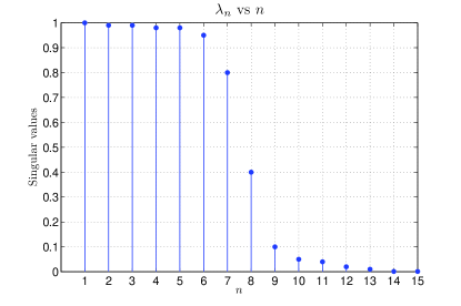
Figure 2: Singular values of an Operator

III-D Computing generalised singular values

Both, degrees of freedom and essential dimension for a communication channel, can be evaluated if the generalised singular values of the operator $T$ describing the channel are known. However, no known method exists for computing these singular values for general compact operators. In this section, we develop a numerical method, based on finite dimensional approximations, that could be used to calculate generalised singular values.

Theorem III.8

Suppose $X$ and $Y$ are normed spaces and $T:X\rightarrow Y$ is a compact operator. Also suppose that $X$ has a complete Schauder basis $\{\phi_{1},\phi_{2},\ldots\}$ and let $S_{n}=\mathrm{span}\{\phi_{1},\ldots,\phi_{n}\}$. Let $T_{n}=T|_{S_{n}}:S_{n}\rightarrow Y$, $n\in\mathbb{Z}^{+}$. If $\epsilon_{m}$, the $m^{th}$ singular value of $T$, exists then for $n$ large enough $\epsilon_{m,n}$, the $m^{th}$ singular value of $T_{n}$, will exist and

$$\lim_{n\rightarrow\infty}\epsilon_{m,n}=\epsilon_{m}.$$

If $\epsilon_{m,n}$ exists then it is a lower bound for $\epsilon_{m}$.

The theorem shows that if the domain of the operator has some complete Schauder basis then we can calculate the generalised singular values of the operator restricted to finite dimensional subspaces and as the subspaces get bigger we will approach the singular values of the original operator. Moreover, the theorem also proves that the singular values of the finite dimensional operators provide lower bounds for the original generalised singular values. We, however, still need a practical method of calculating the singular values of linear operators defined on finite dimensional normed spaces.

Let $X,Y$ be two finite dimensional Banach spaces and let $T:X\rightarrow Y$ be a linear operator. Suppose $\epsilon_{1},\ldots,\epsilon_{n}$ are the generalised singular values of $T$ and denote $B_{1}=\{x\in X:\|x\|_{X}\leq 1\}$. We know that for all $\epsilon\geq\epsilon_{p+1}$, $\mathcal{N}(\epsilon)\leq p$. Hence for each $\epsilon\geq\epsilon_{p+1}$ there exists a set $\{\psi_{i}\}_{i=1}^{p}\subset Y$ such that

$$\sup_{x\in B_{1}}\inf_{a_{1},\ldots,a_{p}}\left\|Tx-\sum_{i=1}^{p}a_{i}\psi_{i}\right\|_{Y}\leq\epsilon.$$

Let $\Psi_{p,\epsilon}$ denote the set of all sets $\{\psi_{i}:\|\psi_{i}\|_{Y}\leq 1\}_{i=1}^{p}\subset Y$ that satisfy the above inequality for a given $\epsilon\geq\epsilon_{p+1}$ and let

$$\Psi_{p}=\bigcup_{\epsilon\geq\epsilon_{p+1}}\Psi_{p,\epsilon}.$$

With this notation we can now prove that the generalised singular values of a linear operator defined on a finite dimensional normed space can be expressed as the solution of an optimisation problem.

Theorem III.9

Let $X,Y$ be two finite dimensional Banach spaces and let $T:X\rightarrow Y$ be a linear operator. Also let $B_{1}$ be the closed unit ball in $X$ and suppose $\Psi_{p}$ is defined as explained above. Then

$$\sup_{x\in B_{1}}\|Tx\|_{Y}=\epsilon_{1}$$

and for all $p\in\mathbb{Z}^{+}$

$$\inf_{\{\psi_{i}\}_{i=1}^{p}\in\Psi_{p}}\sup_{x\in B_{1}}\inf_{a_{1},\ldots,a_{p}}\left\|Tx-\sum_{i=1}^{p}a_{i}\psi_{i}\right\|_{Y}=\epsilon_{p+1}.$$

Given the “correct” set of functions $\psi_{i}$, the above theorem characterises the singular values in terms of a maximisation problem over a finite dimensional domain. It is however difficult to check whether a given set of functions $\{\psi_{i}\}_{i=1}^{p}$ is an element of $\Psi_{p}$. We therefore propose the following algorithm to calculate bounds on the generalised singular values.

Suppose $X,Y$, $T:X\rightarrow Y$, $\epsilon_{1},\ldots,\epsilon_{n}$ and $B_{1}$ are defined as in Theorem III.9. Let

$$\epsilon^{\prime}_{1}=\sup_{x\in B_{1}}\|Tx\|_{Y}.$$

Because $B_{1}\subset X$ is a compact set and $\|\cdot\|_{Y}$ and $T$ are continuous, there exists an $x_{1}\in B_{1}$ such that $\|Tx_{1}\|_{Y}=\epsilon_{1}^{\prime}$. Choose $\psi_{1}=Tx_{1}$.

Now suppose $\psi_{1},\ldots,\psi_{p}$ have been chosen. Then let

$$\epsilon^{\prime}_{p+1}=\sup_{x\in B_{1}}\inf_{a_{1},\ldots,a_{p}}\left\|Tx-\sum_{i=1}^{p}a_{i}\psi_{i}\right\|_{Y}.$$ (2)

Again, because $B_{1}\subset X$ is a compact set and $\|\cdot\|_{Y}$ and $T$ are continuous, there exists an $x_{p+1}\in B_{1}$ such that $x_{p+1}$ attains the maximum in the above equation. Choose $\psi_{p+1}=Tx_{p+1}$. Comparing with Theorem III.9 we note that $\epsilon^{\prime}_{p+1}$ is an upper bound for $\epsilon_{p+1}$. It is an open question as to whether $\epsilon^{\prime}_{p+1}=\epsilon_{p+1}$.

In this algorithm, instead of searching over all possible sets in $\Psi_{p}$ we select a special set that is in some sense (it consists of images of the $x\in B_{1}$ that attain the maximum in equation (2)) the best possible set to use. This choice is essential because otherwise the calculation of generalised singular values becomes too cumbersome (one needs to find the set $\Psi_{p}$ before calculating $\epsilon_{p+1}$). Note however, that the above algorithm gives the correct value for $\epsilon_{1}$.

The theory presented here has been used to compute the generalised singular values and degrees of freedom in spatial waveform channels of the type discussed in Example II.3. The results of these computations are presented in Somaraju [18]. Due to space constraints, these results are not further discussed in this paper.

III-E Non-compactness of channel operators

Throughout this paper we have exclusively dealt with channels that can be modeled using compact operators. We have done so because of the following result.

Theorem III.10

(Converse to Theorem III.1) Suppose $X$ and $Y$ are normed spaces with norms $\|\cdot\|_{X}$ and $\|\cdot\|_{Y}$, respectively, and $T:X\rightarrow Y$ is a bounded linear operator. If for all $\epsilon>0$ there exist $N\in\mathbb{Z}_{0}^{+}$ and a set $\{\psi_{i}\}_{i=1}^{N}\subset Y$ such that for all $x\in\overline{B}_{1,X}(0)$

$$\inf_{a_{1},\ldots,a_{N}}\left\|Tx-\sum_{i=1}^{N}a_{i}\psi_{i}\right\|_{Y}\leq\epsilon$$

then $T$ is compact.

So any bounded channel operator with finitely many sub-channels must be compact. Indeed, if one can find a channel that is not described by a compact operator, then it will have infinitely many sub-channels and will therefore have infinite capacity. Also, if the channel is described by an operator that is linear but unbounded then there will obviously exist sub-channels over which arbitrarily large gains can be obtained.

IV Conclusion

In this paper we assume that a communication channel can be modeled by a normed space $X$ of transmitter functions that a transmitter can generate, a normed space $Y$ of functions that a receiver can measure and an operator $T:X\rightarrow Y$ that maps the transmitter functions to functions measured by the receiver. We then introduce the concepts of degrees of freedom at level $\epsilon$, essential dimension and generalised singular values of such channel operators in the case where they are compact. One can give a physical interpretation for degrees of freedom as follows: if there is some constraint $\|\cdot\|_{X}\leq 1$ on the space of source functions and if the receiver can only measure signals that satisfy $\|\cdot\|_{Y}>\epsilon$ then the number of degrees of freedom is the number of linearly independent signals that the receiver can measure under the given constraints. If the degrees of freedom are largely independent of the level $\epsilon$ then it makes sense to talk about the essential dimension of the channel. The essential dimension of the channel is the smallest number of degrees of freedom of the channel that is the same for the largest range of levels $\epsilon$. We show how one can use the number of degrees of freedom at level $\epsilon$ to generalise the Hilbert space concept of singular values to arbitrary normed spaces. We also provide a simple algorithm that can be used to approximately calculate these generalised singular values. Finally, we prove that if the operator describing the channel is not compact then it must either have infinite gain or have an infinite number of degrees of freedom. The general theory developed in this paper is applied to spatial waveform channels in Somaraju [18].

Proofs of Theorems: Theorem III.1. Suppose $X$ and $Y$ are normed spaces with norms $\|\cdot\|_{X}$ and $\|\cdot\|_{Y}$, respectively, and $T:X\rightarrow Y$ is a compact operator. Then for all $\epsilon>0$ there exist $N\in\mathbb{Z}_{0}^{+}$ and a set $\{\psi_{i}\}_{i=1}^{N}\subset Y$ such that for all $x\in\overline{B}_{1,X}(0)$

$$\inf_{a_{1},\ldots,a_{N}}\left\|Tx-\sum_{i=1}^{N}a_{i}\psi_{i}\right\|_{Y}\leq\epsilon.$$ (3)

Proof:

The proof is by contradiction. Let $\epsilon>0$ be given. Suppose no such $N$ exists.

Let $x_{1}\in\overline{B}_{1,X}(0)$ be any vector. Choose $\psi_{1}=Tx_{1}$. Suppose that $\{x_{1},\ldots,x_{N}\}$ and $\{\psi_{1},\ldots,\psi_{N}\}$ have been chosen. Then, by our assumption, there exists an $x_{N+1}\in\overline{B}_{1,X}(0)$ such that

$$\inf_{a_{1},\ldots,a_{N}}\left\|Tx_{N+1}-\sum_{i=1}^{N}a_{i}\psi_{i}\right\|_{Y}>\epsilon.$$ (4)

Choose $\psi_{N+1}=Tx_{N+1}$. By induction, for $M\leq N$ we have

$$\|Tx_{N+1}-Tx_{M}\|_{Y}>\epsilon.$$

This follows from (4) by setting $a_{i}=0$, $i\leq N$, $i\neq M$, and $a_{M}=1$. Therefore, using the Cauchy criterion, the sequence $\{Tx_{n}\}_{n=1}^{\infty}$ chosen by induction cannot have a convergent subsequence. This is the required contradiction because $\{x_{n}\}_{n=1}^{\infty}$ is a bounded sequence and $T$ is compact. ∎

Theorem III.2. Suppose $X$ and $Y$ are normed spaces with norms $\|\cdot\|_{X}$ and $\|\cdot\|_{Y}$, respectively, and $T:X\rightarrow Y$ is a compact operator. Let $\mathcal{N}(\epsilon)$ denote the number of degrees of freedom of $T$ at level $\epsilon$. Then

1. $\mathcal{N}(\epsilon)=0$ for all $\epsilon\geq\|T\|$.

2. Unless $T$ is identically zero, there exists an $\epsilon_{0}>0$ such that $\mathcal{N}(\epsilon)\geq 1$ for all $0<\epsilon<\epsilon_{0}$.

3. $\mathcal{N}(\epsilon)$ is a non-increasing, upper semicontinuous function of $\epsilon$.

4. In any finite interval $(\epsilon_{1},\epsilon_{2})\subset\mathbb{R}$, with $0<\epsilon_{1}<\epsilon_{2}$, $\mathcal{N}(\epsilon)$ has only finitely many discontinuities, i.e. $\mathcal{N}(\epsilon)$ only takes finitely many non-negative integer values in any finite $\epsilon$ interval.

Proof:

1. Because $T$ is compact it is bounded, and therefore $\|T\|<\infty$. Suppose $\epsilon\geq\|T\|$ then $\|Tx\|_{Y}\leq\|T\|\leq\epsilon$ for all $x\in\overline{B}_{1,X}(0)$. Therefore $\mathcal{N}(\epsilon)=0$.

2. If $\|T\|>0$ there exists an $x\in X$, $\|x\|_{X}\leq 1$ such that $\|Tx\|_{Y}>0$. Set $\epsilon_{0}:=\|Tx\|_{Y}$. Then for all $0<\epsilon<\epsilon_{0}$, $\mathcal{N}(\epsilon)\geq 1$.

3. Suppose $0<\epsilon_{1}<\epsilon_{2}$. Then there exist functions $\psi_{1},\ldots,\psi_{\mathcal{N}(\epsilon_{1})}$ such that for all $x\in\overline{B}_{1,X}(0)$

   $$\inf_{a_{1},\ldots,a_{\mathcal{N}(\epsilon_{1})}}\left\|Tx-\sum_{i=1}^{\mathcal{N}(\epsilon_{1})}a_{i}\psi_{i}\right\|_{Y}<\epsilon_{1}<\epsilon_{2}$$

   Therefore $\mathcal{N}(\epsilon_{2})\leq\mathcal{N}(\epsilon_{1})$ from the definition of the number of degrees of freedom at level $\epsilon$, i.e. $\mathcal{N}(\epsilon)$ is non-increasing. In particular we have

   $$\lim_{\epsilon\searrow\epsilon_{1}}\mathcal{N}(\epsilon)\leq\mathcal{N}(\epsilon_{1}).$$

   Assume that the above inequality is strict. Then there exists an $N\in\mathbb{Z}_{0}^{+}$, $N<\mathcal{N}(\epsilon_{1})$, and for all $\theta>0$ there exists a set $\{\psi_{i}^{\theta}\}_{i=1}^{N}\subset Y$ such that for all $x\in\overline{B}_{1,X}(0)$

   $$\inf_{a_{1},\ldots,a_{N}}\left\|Tx-\sum_{i=1}^{N}a_{i}\psi_{i}^{\theta}\right\|_{Y}\leq\epsilon_{1}+\theta.$$ (5)

   On the other hand, since $\mathcal{N}(\epsilon_{1})>N$, for all sets $\{\psi_{i}\}_{i=1}^{N}\subset Y$ there exists an $x\in\overline{B}_{1,X}(0)$ such that

   $$\mu:=\inf_{a_{1},\ldots,a_{N}}\left\|Tx-\sum_{i=1}^{N}a_{i}\psi_{i}\right\|_{Y}>\epsilon_{1}.$$ (6)

   But (5) contradicts (6) for $\theta:=\frac{1}{2}(\mu-\epsilon_{1})$. Hence $\lim_{\epsilon\searrow\epsilon_{1}}\mathcal{N}(\epsilon)=\mathcal{N}(\epsilon_{1})$ and $\mathcal{N}(\epsilon)$ is upper semicontinuous.

4. This follows from Parts 1 and 3.

∎

Proposition III.3. Suppose $X$ and $Y$ are normed spaces and $T:X\rightarrow Y$ is a compact operator. Let $\mathcal{N}(\epsilon)$ denote the number of degrees of freedom of $T$ at level $\epsilon$. Then $\mathcal{N}(\epsilon)$ is equal to the number of generalised singular values that are greater than $\epsilon$.

Proof:

This follows from careful counting of the numbers of degrees of freedom at level $\epsilon$ including repeated counting according to the height of any occurring “jumps”. ∎

Theorem III.4. Suppose $X$ and $Y$ are normed spaces with norms $\|\cdot\|_{X}$ and $\|\cdot\|_{Y}$, respectively, and $T:X\rightarrow Y$ is a compact operator. Let $\epsilon_{m}$ be a generalised singular value of the operator $T$. Then for all $\theta>0$ there exists a $\phi\in X$, $\|\phi\|_{X}=1$, such that

$$\epsilon_{m}+\theta\geq\|T\phi\|_{Y}\geq\epsilon_{m}-\theta.$$

Proof:

The proof is by contradiction. Assume that there exists a $\theta>0$ such that for all $\phi\in X$, $\|\phi\|_{X}=1$, we have $\|T\phi\|_{Y}\notin[\epsilon_{m}-\theta,\epsilon_{m}+\theta]$. Let $\mathcal{N}(\epsilon)$ denote the number of degrees of freedom at level $\epsilon$ of the operator $T$. From the definition of degrees of freedom at level $\epsilon$ we have

$$\mathcal{N}(\epsilon_{m}+\theta) \leq m-1,$$ (7)

$$\mathcal{N}(\epsilon_{m}-\theta) \geq m.$$ (8)

By (7), there exist vectors $\psi_{1},\ldots,\psi_{m-1}\in Y$ such that for all $x\in\overline{B}_{1,X}(0)$

$$\inf_{a_{1},\ldots,a_{m-1}}\left\|Tx-\sum_{i=1}^{m-1}a_{i}\psi_{i}\right\|\leq\epsilon_{m}+\theta.$$

By our assumption on $\|T\phi\|_{Y}$,

$$\inf_{a_{1},\ldots,a_{m-1}}\left\|T\phi-\sum_{i=1}^{m-1}a_{i}\psi_{i}\right\|\leq\epsilon_{m}-\theta.$$

This follows from consideration of the case $a_{1}=\dots=a_{m-1}=0$. Hence $\mathcal{N}(\epsilon_{m}-\theta)\leq m-1$ since scaling $\phi$ to non-unit norm is equivalent to scaling all the $a_{i}$. This contradicts inequality (8). Therefore there exists a $\phi$ that satisfies the conditions of the theorem. ∎

Theorem III.5. Suppose $\mathcal{H}_{1}$ and $\mathcal{H}_{2}$ are Hilbert spaces and $T:\mathcal{H}_{1}\rightarrow\mathcal{H}_{2}$ is a compact operator. Then for all $\epsilon>0$ there exist an $N\in\mathbb{Z}^{+}_{0}$ and a set of $N$ mutually orthogonal vectors $\{\phi_{i}\}^{N}_{i=1}\subset\mathcal{H}_{1}$ such that if

$$x\in\mathcal{H}_{1},\ \|x\|_{\mathcal{H}_{1}}\leq 1\textrm{ and }\langle x,\phi_{i}\rangle_{\mathcal{H}_{1}}=0$$

then

$$\|Tx\|_{\mathcal{H}_{2}}\leq\epsilon.$$

Moreover, the smallest $N$ that satisfies the above condition for a given $\epsilon$ is equal to the number of Hilbert space singular values of $T$ that are greater than $\epsilon$.

Proof:

We first prove that such an $N$ is given by the number of Hilbert space singular values of $T$ that are greater than $\epsilon$ and then prove that this is the smallest such $N$.

Let $\epsilon>0$ be given. Because $T$ is compact, we can use the singular value decomposition theorem which says [21, p. 261]

$$T\cdot=\sum_{i}\sigma_{i}\langle\cdot,\phi_{i}\rangle_{\mathcal{H}_{1}}\psi_{i}.$$ (9)

Here, $\sigma_{i}$, $\phi_{i}$ and $\psi_{i}$ with $i\in\mathbb{Z}^{+}$ are the Hilbert space singular values and left and right singular vectors of $T$, respectively. We assume w.l.o.g. that the Hilbert space singular values are ordered in non-increasing order. We denote by $N_{1}\in\mathbb{Z}^{+}$ the number of Hilbert space singular values of $T$ that are greater than $\epsilon$, i.e. $\sigma_{i}>\epsilon$ if and only if $i\leq N_{1}$.

Now, if $x$ is orthogonal to $\phi_{i},i=1,\ldots,N_{1}$ and if $\|x\|_{\mathcal{H}_{1}}\leq 1$ then from equation (9)

$$\|Tx\|_{\mathcal{H}_{2}}^{2} = \sum_{i=1}^{\infty}\sigma_{i}^{2}|\langle x,\phi_{i}\rangle_{\mathcal{H}_{1}}|^{2}\|\psi_{i}\|_{\mathcal{H}_{2}}^{2}$$

$$\leq \epsilon^{2}\sum_{i=N_{1}+1}^{\infty}|\langle x,\phi_{i}\rangle_{\mathcal{H}_{1}}|^{2}$$

$$\leq \epsilon^{2}.$$

For $N<N_{1}$, the linear span of any set $\{\varphi_{i}\}_{i=1}^{N}\subset\mathcal{H}_{1}$ has a non-trivial orthogonal complement in the span of $\{\phi_{i}\}_{i=1}^{N_{1}}$. Any vector $x$ in this complement with $\|x\|_{\mathcal{H}_{1}}=1$ fullfills the conditions of the theorem but $\|Tx\|_{\mathcal{H}_{2}}>\epsilon$ by equation (9). ∎

Theorem III.6. Suppose that $\mathcal{H}_{1}$ and $\mathcal{H}_{2}$ are Hilbert spaces and $T:\mathcal{H}_{1}\rightarrow\mathcal{H}_{2}$ is a compact operator. Then the number of degrees of freedom at level $\epsilon$ is equal to the number of Hilbert space singular values of $T$ that are greater than $\epsilon$.

Proof:

As in the prove of the previous theorem, let $N_{1}\in\mathbb{Z}^{+}$ denote the number of Hilbert space singular values of $T$ that are greater than $\epsilon$. Let $\sigma_{i}$, $\phi_{i}$ and $\psi_{i}$ with $i\in\mathbb{Z}^{+}$ denote the Hilbert space singular values in non-increasing order and the left and right singular vectors of $T$, respectively. Let $N_{2}\in\mathbb{Z}^{+}$ denote the number of degrees of freedom of $T$ at level $\epsilon$.

We first prove that $N_{1}\geq N_{2}$. If $x$ is in the unit ball in ${\mathcal{H}_{1}}$ then we can write $x=\sum_{i=1}^{\infty}\langle x,\phi_{i}\rangle_{\mathcal{H}_{1}}\phi_{i}+x_{r}$. Here $x_{r}$ is the remainder term that is orthogonal to all the $\phi_{i}$. From equation (9) and $\sigma_{i}\leq\epsilon$ for $i>N_{1}$ it follows that

$$\left\|Tx-\sum_{i=1}^{N_{1}}\sigma_{i}\langle x,\phi_{i}\rangle_{\mathcal{H}_{1}}\psi_{i}\right\|_{\mathcal{H}_{2}}\leq\epsilon$$

and hence $N_{1}\geq N_{2}$ by the definition of the number of degrees of freedom at level $\epsilon$ (set $a_{i}=\sigma_{i}\langle x,\phi_{i}\rangle_{\mathcal{H}_{1}}$ in that definition).

To prove that $N_{1}\leq N_{2}$ assume that $N_{1}>N_{2}$ to arrive at a contradiction. Then there exists a set $\{\psi_{i}^{\prime}\}_{i=1}^{N_{2}}\subset\mathcal{H}_{2}$ such that

$$\inf_{a_{1},\ldots,a_{N_{2}}}\left\|Tx-\sum_{i=1}^{N_{2}}a_{i}\psi^{\prime}_{i}\right\|_{\mathcal{H}_{2}}\leq\epsilon$$

for all $x\in\mathcal{H}_{1}$, $\|x\|_{\mathcal{H}_{1}}\leq 1$. Because we assume that $N_{1}>N_{2}$, there exists a $y\in\mathrm{span}\{\psi_{1},\ldots,\psi_{N_{1}}\}$ which is orthogonal to all the $\psi_{i}^{\prime}$. Let $y=\sum_{i=1}^{N_{1}}b_{i}\psi_{i}$. Then $y=Tx$ where $x=\sum_{i=1}^{N_{1}}\frac{b_{i}}{\sigma_{i}}\phi_{i}$ by equation (9). We can assume w.l.o.g. that the $b_{i}$ are normalised so that $\|x\|_{\mathcal{H}_{1}}=1$. If this is done then

$$\inf_{a_{1},\ldots,a_{N_{2}}}\left\|Tx-\sum_{i=1}^{N_{2}}a_{i}\psi^{\prime}_{i}\right\|^{2}_{\mathcal{H}_{2}} = \|y\|_{\mathcal{H}_{2}}^{2}$$ (10)

$$= \sum_{i=1}^{N_{1}}b_{i}^{2}$$ (11)

$$> \sum_{i=1}^{N_{1}}\frac{b_{i}^{2}}{\sigma_{i}^{2}}\epsilon^{2}$$ (12)

$$= \epsilon^{2}.$$ (13)

In the above we get equation (10) from the fact that $y$ is orthogonal to all the $\psi_{i}^{\prime}$, inequality (12) from $\sigma_{i}>\epsilon$ for $i\leq N_{1}$ and equation (13) from $\|x\|_{\mathcal{H}_{1}}=1$. The inequality (10)–(13) is the required contradiction. This proves that $N_{1}\leq N_{2}$ and hence $N_{1}=N_{2}$. ∎

Corollary III.1. Suppose $\mathcal{H}_{1}$ and $\mathcal{H}_{2}$ are Hilbert spaces and $T:\mathcal{H}_{1}\rightarrow\mathcal{H}_{2}$ is a compact operator. Suppose $\{\epsilon_{m}\}$ are the generalised singular values of $T$ and $\{\sigma_{m}\}$ are the possibly repeated Hilbert space singular values of $T$ written in non-increasing order. Then

$$\sigma_{m}=\epsilon_{m}$$

for all $m\in\mathbb{Z}^{+}$.

Proof:

This follows immediately from Theorem III.6 and Proposition III.3 by a simple counting argument. ∎

Theorem III.8. Suppose $X$ and $Y$ are normed spaces and $T:X\rightarrow Y$ is a compact operator. Also suppose that $X$ has a complete Schauder basis $\{\phi_{1},\phi_{2},\ldots\}$ and let $S_{n}=\mathrm{span}\{\phi_{1},\ldots,\phi_{n}\}$. Let $T_{n}=T|_{S_{n}}:S_{n}\rightarrow Y$, $n\in\mathbb{Z}^{+}$. If $\epsilon_{m}$, the $m^{th}$ singular value of $T$, exists then for $n$ large enough $\epsilon_{m,n}$, the $m^{th}$ singular value of $T_{n}$, will exist and

$$\lim_{n\rightarrow\infty}\epsilon_{m,n}=\epsilon_{m}.$$

If $\epsilon_{m,n}$ exists then it is a lower bound for $\epsilon_{m}$.
Proof Outline: The crux of the argument used to prove the theorem is as follows. Assume $\epsilon>0$ is given and let $\mathcal{N}(\epsilon)$ denote the number of degrees of freedom at level $\epsilon$ for the operator $T$. By definition there exist functions $\{\psi_{1},\ldots,\psi_{\mathcal{N}(\epsilon)}\}\subset Y$ such that for all $x\in X$, $\|x\|_{X}\leq 1$, $Tx$ can be approximated to level $\epsilon$ by a linear combination of the $\psi_{i}$ and further, no set of functions $\{\psi^{\prime}_{1},\ldots,\psi^{\prime}_{N}\}\subset Y$ can approximate all the $Tx$ if $N<\mathcal{N}(\epsilon)$. Equivalently, there is a vector in the closed unit ball in $X$ whose image under $T$ can be approximated by a vector in $\mathrm{span}\{\psi_{1},\ldots,\psi_{\mathcal{N}(\epsilon)}\}$ but not by any vector in $\mathrm{span}\{\psi^{\prime}_{1},\ldots,\psi^{\prime}_{N}\}$.

So we take the inverse image of an $\epsilon$-net of points in $\mathrm{span}\{\psi_{1},\ldots,\psi_{\mathcal{N}(\epsilon)}\}$ and choose $n$ large enough so that all the inverse images are close to $S_{n}$. We can do this because the $\phi_{i}$ form a complete Schauder basis for $X$. We then show that there exists a vector in $S_{n}$ such that its image under $T$ cannot be approximated by a linear combination of $\psi^{\prime}_{1},\ldots,\psi^{\prime}_{N}$ for $N<\mathcal{N}(\epsilon)$. This will prove that the number of degrees of freedom at level $\epsilon$ of $T_{n}$ approaches that of $T$ and consequently so do the singular values. The details are as follows.

Proof:

We will prove this theorem in two parts. Assume that $\epsilon_{m}$ exists. In part a) we will prove that if $\epsilon_{m,N}$ exists for some $N\in\mathbb{Z}^{+}$ then $\epsilon_{m,n}$ exists for all $n>N$, and the $\epsilon_{m,n}$ form a non-decreasing sequence indexed by $n$ that is bounded from above by $\epsilon_{m}$. In part b) we prove by contradiction that $\epsilon_{m,n}$ exists for some $n\in\mathbb{Z}^{+}$ and that $\epsilon_{m,n}$ must converge to $\epsilon_{m}$.

We will use the following notation in the proof:

$$\mathrm{span}_{\epsilon}\{\psi_{1},\ldots,\psi_{N}\}=\\ \{y\in Y:\inf_{a_{1},\ldots,a_{N}}\left\|y-\sum_{i=1}^{N}a_{i}\psi_{i}\right\|_{Y}\leq\epsilon\}$$

and $B_{r}=\{x\in X:\|x\|_{X}\leq r\}$.

Part a: Let $T$ and $T_{n}$ be defined as in the theorem and let $\mathcal{N}(\epsilon)$ and $\mathcal{N}_{n}(\epsilon)$ be the numbers of degrees of freedom at level $\epsilon$ of $T$ and $T_{n}$, respectively. Assume that $\epsilon_{m,n_{1}}$ exists and let $n_{2}>n_{1}$.

Then for all sets $\{\psi_{1},\ldots,\psi_{\mathcal{N}_{n_{1}}(\epsilon)-1}\}\subset Y$ there is a $\xi\in S_{n_{1}}\cap B_{1}$ such that

$$T_{n_{1}}\xi=T\xi\notin\mathrm{span}_{\epsilon}\{\psi_{1},\ldots,\psi_{\mathcal{N}_{n_{1}}(\epsilon)-1}\}.$$

Because $S_{n_{1}}\subset S_{n_{2}}$ we have $\xi\in S_{n_{2}}\cap B_{1}$ and

$$T_{n_{2}}\xi=T\xi\notin\mathrm{span}_{\epsilon}\{\psi_{1},\ldots,\psi_{\mathcal{N}_{n_{1}}(\epsilon)-1}\}.$$

Therefore for all $\epsilon>0$

$$\mathcal{N}_{n_{2}}(\epsilon)\geq\mathcal{N}_{n_{1}}(\epsilon).$$ (14)

Because

$$\inf_{\epsilon<\epsilon_{m,n_{1}}}\mathcal{N}_{n_{1}}(\epsilon)\geq m$$ (15)

we have $\mathcal{N}_{n_{2}}(\epsilon)\geq\mathcal{N}_{n_{1}}(\epsilon)\geq m$ for $\epsilon<\epsilon_{m,n_{1}}$. Hence $\epsilon_{m,n_{2}}$ must exist.

From the definition of generalised singular values we have inequality (15) and

$$\sup_{\epsilon>\epsilon_{m,n_{2}}}\mathcal{N}_{n_{2}}(\epsilon)\leq m-1$$

If $\epsilon_{m,n_{1}}>\epsilon_{m,n_{2}}$ then there exists an $\epsilon^{\prime}$ such that $\epsilon_{m,n_{1}}>\epsilon^{\prime}>\epsilon_{m,n_{2}}$. Therefore,

$$\mathcal{N}_{n_{1}}(\epsilon^{\prime})\geq m>m-1\geq\mathcal{N}_{n_{2}}(\epsilon^{\prime}).$$

This contradicts inequality (14). Therefore $\epsilon_{m,n_{1}}\leq\epsilon_{m,n_{2}}$.

The same line of arguments as above can be used to show that if both $\epsilon_{m}$ and $\epsilon_{m,n}$ exist then $\epsilon_{m,n}\leq\epsilon_{m}$. Recall that we have assumed at the beginning that $\epsilon_{m}$ exists. Therefore, if $\epsilon_{m,N}$ exists for some $N\in\mathbb{Z}^{+}$ then $\epsilon_{m,n}$ is a non-decreasing sequence in $n\geq N$ that is bounded from above by $\epsilon_{m}$.
Part b: By part a), if $\epsilon_{m,n}$ exists for $n\geq n_{1}$ then, because $\epsilon_{m,n}$ is a bounded monotonic sequence in $n$ it must converge to some $\epsilon_{m}^{\prime}\leq\epsilon_{m}$.

Now there are two situations to consider. Firstly, $\epsilon_{m,n}$ might not exist for any $n\in\mathbb{Z}^{+}$. Secondly, $\epsilon_{m,n}$ might exist for some $n$ but the limit $\epsilon_{m}^{\prime}$ might be strictly less than $\epsilon_{m}$. We consider the two situations separately and arrive at the same set of inequalities in both situations. We then derive a contradiction from that set.

Situation 1: Assume that $\epsilon_{m,n}$ does not exist for any $n\in\mathbb{Z}^{+}$. Then

$$\mathcal{N}_{n}(\epsilon)\leq m-1$$ (16)

for all $n\in\mathbb{Z}^{+}$ and $\epsilon>0$. Using the definition of degrees of freedom for $T$ there exist constants $\alpha<\beta<\epsilon_{m}$ such that

$$\mathcal{N}_{n}(\alpha)\leq m-1 \quad\textrm{for all }n\in\mathbb{Z}^{+}\quad\textrm{and}$$ (17)

$$\mathcal{N}(\beta)\geq m.$$ (18)

Situation 2: Assume that $\epsilon_{m}^{\prime}<\epsilon_{m}$. From the definition of generalised singular values we know

$$\sup_{\epsilon>\epsilon_{m,n}}\mathcal{N}_{n}(\epsilon)\leq m-1 \ \textrm{for all }n\in\mathbb{Z}^{+}\quad\textrm{and}$$

$$\inf_{\epsilon<\epsilon_{m}}\mathcal{N}(\epsilon)\geq m.$$

Because $\epsilon_{m,n}\leq\epsilon^{\prime}_{m}$, we know that there exist numbers $\alpha$ and $\beta$, $\epsilon^{\prime}_{m}<\alpha<\beta<\epsilon_{m}$ such that

$$\mathcal{N}_{n}(\alpha)\leq m-1 \ \textrm{for all }n\in\mathbb{Z}^{+}\quad\textrm{and}$$ (19)

$$\mathcal{N}(\beta)\geq m.$$ (20)

These are the same conditions as (17) and (18). Therefore, in both situations we need to prove that the inequalities (19) and (20) cannot be simultaneously true.

Because $T$ is compact, $TB_{1}$ is totally bounded [20, ch. 8]. Therefore, $TB_{1}$ has a finite $\epsilon$-net for all $\epsilon>0$. Hence there exists a set of vectors $\{\xi_{1},\ldots,\xi_{P}\}\subset B_{1}$ such that for all $y\in TB_{1}$ there exists a $p$, $1\leq p\leq P$ with

$$\|T\xi_{p}-y\|_{Y}<\frac{\beta-\alpha}{2}.$$ (21)

Now, because $\{\phi_{1},\phi_{2},\ldots\}$ is a complete Schauder basis for $X$ and because $P<\infty$, there exists a number $N$ such that for all $n>N$ and for all $p$, $1\leq p\leq P$, there exists a $\xi_{p,n}\in S_{n}\cap B_{1}$ such that

$$\|\xi_{p,n}-\xi_{p}\|_{X}<\frac{\beta-\alpha}{2\|T\|}.$$ (22)

Therefore, for all $y\in TB_{1}$ and for all $n>N$ there exists a $p,1\leq p\leq P$ and a $\xi_{p,n}\in S_{n}\cap B_{1}$ such that

$$\|T\xi_{p,n}-y\|_{Y} = \|T\xi_{p,n}-T\xi_{p}+T\xi_{p}-y\|_{Y}$$ (23)

$$\leq \|T\xi_{p,n}-T\xi_{p}\|_{Y}+\|T\xi_{p}-y\|_{Y}$$

$$< \|T(\xi_{p,n}-\xi_{p})\|_{Y}+\frac{\beta-\alpha}{2}$$

$$< \|T\|\frac{\beta-\alpha}{2\|T\|}+\frac{\beta-\alpha}{2}$$

$$= \beta-\alpha.$$

We get the first inequality above from the triangle inequality, the second one from inequality (21) and the final one from inequality (22). From inequality (19) and the definition of the number of degrees of freedom, we know that for all $n\in\mathbb{Z}^{+}$ there exists a set of vectors $\{\psi_{1,n},\ldots,\psi_{m-1,n}\}\subset Y$ such that

$$y\in\mathrm{span}_{\alpha}\{\psi_{1,n},\ldots,\psi_{m-1,n}\}$$ (24)

for all $y\in T(S_{n}\cap B_{1})$.

But, from the definition of the number of degrees of freedom and inequality (20) we know that for all $n\in\mathbb{Z}^{+}$ and all sets of vectors $\{\psi_{1,n},\ldots,\psi_{m-1,n}\}$ there exists a vector $\psi\in TB_{1}$ such that

$$\psi\notin\mathrm{span}_{\beta}\{\psi_{1,n},\ldots,\psi_{m-1,n}\}.$$

From inequality (23) we know that for all $n>N$ there exists a $\xi_{p,n}\in S_{n}\cap B_{1}$ such that

$$\|T\xi_{p,n}-\psi\|<\beta-\alpha.$$

Therefore, for all $n>N$ there exists a $\xi_{p,n}\in S_{n}\cap B_{1}$ such that

$$T\xi_{p,n}\notin\mathrm{span}_{\alpha}\{\psi_{1,n},\ldots,\psi_{m-1,n}\}.$$ (25)

This directly contradicts condition (24). Therefore, if $\epsilon_{m}$ exists then $\epsilon_{m,n}$ exists for $n$ large enough and

$$\lim_{n\rightarrow\infty}\epsilon_{m,n}=\epsilon_{m}.$$

∎

Theorem III.9. Let $X,Y$ be two finite dimensional Banach spaces and let $T:X\rightarrow Y$ be a linear operator. Also let $B_{1}$ be the closed unit ball in $X$ and suppose $\Psi_{p}$ is defined as in Section III-D. Then

$$\sup_{x\in B_{1}}\|Tx\|_{Y}=\epsilon_{1}$$

and for all $p\in\mathbb{Z}^{+}$

$$\inf_{\{\psi_{i}\}_{i=1}^{p}\in\Psi_{p}}\sup_{x\in B_{1}}\inf_{a_{1},\ldots,a_{p}}\left\|Tx-\sum_{i=1}^{p}a_{i}\psi_{i}\right\|_{Y}=\epsilon_{p+1}.$$

Proof:

Let $\epsilon_{p+1}^{\prime}$ denote the left hand side of the above equation. Assume $\epsilon_{p+1}^{\prime}<\epsilon_{p+1}$. Then there exists a set $\{\psi_{i}\}_{i=1}^{p}\in\Psi_{p}$ such that

$$\epsilon_{p+1}^{\prime\prime}:=\sup_{x\in B_{1}}\inf_{a_{1},\dots,a_{p}}\left\|Tx-\sum_{i=1}^{p}a_{i}\psi_{i}\right\|<\epsilon_{p+1}.$$

By definition this implies $\mathcal{N}(\epsilon_{p+1}^{\prime\prime})\leq p$, a contradiction to $\inf_{\epsilon<\epsilon_{p+1}}\mathcal{N}(\epsilon)\geq p+1$. Hence $\epsilon_{p+1}^{\prime}\geq\epsilon_{p+1}$. Now assume $\epsilon_{p+1}^{\prime}>\epsilon_{p+1}$. Let $\epsilon\in(\epsilon_{p+1},\epsilon^{\prime}_{p+1})$. From $\sup_{\epsilon>\epsilon_{p+1}}\mathcal{N}(\epsilon)=p$ it follows $\mathcal{N}(\epsilon)\leq p$. Hence there exists a set $\{\psi_{i}\}_{i=1}^{p}\subset Y$ such that

$$\sup_{x\in B_{1}}\inf_{a_{1},\dots,a_{p}}\left\|Tx-\sum_{i=1}^{p}a_{i}\psi_{i}\right\|\leq\epsilon<\epsilon^{\prime}_{p+1}.$$

Therefore $\{\psi_{i}\}_{i=1}^{p}\in\Psi_{p,\epsilon}\subset\Psi_{p}$ and

$$\epsilon_{p+1}^{\prime}>\inf_{\{\psi_{i}\}_{i=1}^{p}\in\Psi_{p}}\sup_{x\in B_{1}}\inf_{a_{1},\dots,a_{p}}\left\|Tx-\sum_{i=1}^{p}a_{i}\psi_{i}\right\|,$$

a contradiction. Hence $\epsilon_{p+1}^{\prime}=\epsilon_{p+1}$. ∎

Theorem III.10. (Converse to Theorem III.1) Suppose $X$ and $Y$ are normed spaces with norms $\|\cdot\|_{X}$ and $\|\cdot\|_{Y}$, respectively, and $T:X\rightarrow Y$ is a bounded linear operator. If for all $\epsilon>0$ there exist $N\in\mathbb{Z}_{0}^{+}$ and a set $\{\psi_{i}\}_{i=1}^{N}\subset Y$ such that for all $x\in\overline{B}_{1,X}(0)$

$$\inf_{a_{1},\ldots,a_{N}}\left\|Tx-\sum_{i=1}^{N}a_{i}\psi_{i}\right\|_{Y}\leq\epsilon$$

then $T$ is compact.

Proof:

We prove that $T$ is compact by showing that the set $T(\overline{B}_{1,X}(0))$ is totally bounded. Let $\delta>0$ be given. Then there exist an $N\in\mathbb{Z}_{0}^{+}$ and a set $\{\psi_{i}\}_{i=1}^{N}\subset Y$ such that for all $x\in\overline{B}_{1,X}(0)$

$$\inf_{a_{1},\ldots,a_{N}}\left\|Tx-\sum_{i=1}^{N}a_{i}\psi_{i}\right\|_{Y}\leq\frac{\delta}{4}.$$ (26)

For any given $x\in\overline{B}_{1,X}(0)$ we can choose ${a}_{i}^{x}$, $i=1,\ldots,N$ such that

$$\left\|Tx-\sum_{i=1}^{N}{a}_{i}^{x}\psi_{i}\right\|_{Y}$$ (27)

$$\leq \inf_{a_{1},\ldots,a_{N}}\left\|Tx-\sum_{i=1}^{N}a_{i}\psi_{i}\right\|_{Y}+\frac{\delta}{4}$$

$$\leq \frac{\delta}{2}.$$ (28)

Here, the last inequality follows from (26). Also, because we can choose $a_{i}=0$ for $i=1,\ldots,N$, for all $x\in\overline{B}_{1,X}(0)$

$$\inf_{a_{1},\ldots,a_{N}}\left\|Tx-\sum_{i=1}^{N}a_{i}\psi_{i}\right\|_{Y}\leq\|Tx\|_{Y}.$$ (29)

Substituting inequality (29) into (27) and using the triangle inequality, we get

$$\left\|\sum_{i=1}^{N}{a}_{i}^{x}\psi_{i}\right\|_{Y}\leq 2\|Tx\|_{Y}+\frac{\delta}{4}\leq 2\|T\|+\frac{\delta}{4}.$$ (30)

We get the last inequality from the boundedness of $T$. Because the span of $\psi_{1},\ldots,\psi_{N}$ is finite dimensional and because of the uniform bound (30), there exists a finite set of elements $\{y_{1},\ldots,y_{M}\}\subset Y$ such that for all $x\in\overline{B}_{1,X}(0)$

$$\inf_{i=1,\ldots,M}\left\|y_{i}-\sum_{j=1}^{N}{a}_{j}^{x}\psi_{j}\right\|_{Y}\leq\frac{\delta}{2}.$$ (31)

From inequalities (31) and (28) and the triangle inequality we get for all $x\in\overline{B}_{1,X}(0)$

$$\inf_{i=1,\ldots,M}\|y_{i}-Tx\|_{Y}\leq\delta.$$ (32)

Therefore, the $y_{i}$, $i=1,\ldots,M$ form a finite $\delta$-net for $T(\overline{B}_{1,X}(0))$ and therefore $T(\overline{B}_{1,X}(0))$ is totally bounded. Hence, $T$ is compact. ∎

References

- [1] C. E. Shannon, “A mathematical theory of communication,” Bell Syst. Tech. J., vol. 27, pp. 379–423, 1948.
- [2] R. Gallagher, Information Theory and Reliable Communication. New York, USA: John Wiley & Sons, 1968.
- [3] S. Verdú, “Fifty years of Shannon theory,” IEEE Transactions on Information Theory, vol. 44, no. 6, p. 2057, 1998.
- [4] H. Landau and H. Pollak, “Prolate spheroidal wave functions, Fourier analysis and uncertainty - III: The dimension of the space of essentially time- and band-limited signals,” The Bell System Technical Journal, vol. 41, pp. 1295–1336, Jul 1962.
- [5] E. Biglieri and G. Taricco, Transmission and Reception with Multiple Antennas: Theoretical Foundations, ser. Foundations and Trends in Communications and Information Theory. Now Publishers, 2004.
- [6] H. Bölcskei, D. Gesbert, and A. J. Paulraj, “On the capacity of OFDM-based spatial multiplexing systems,” IEEE Transactions on Communications, vol. 50, no. 2, p. 225, 2002.
- [7] A. Grant and P. D. Alexander, “Random sequence multisets for synchronous code-division multiple-access channels,” IEEE Transactions on Information Theory, vol. 44, no. 7, p. 2832, 1998.
- [8] A. M. Tulino and S. Verdú, Random Matrix Theory and Wireless Communications, ser. Foundations and Trends in Communications and Information Theory. Now Publishers, 2004.
- [9] A. S. Y. Poon, R. W. Brodersen, and D. N. C. Tse, “Degrees of freedom in multiple-antenna channels: A signal space approach,” IEEE Transactions on Information Theory, vol. 51, no. 2, pp. 523–536, February 2005.
- [10] L. Hanlen and M. Fu, “Wireless communication systems with spatial diversity: A volumetric model,” IEEE Transactions on Wireless Communications, vol. 5, no. 1, pp. 133–142, January 2006.
- [11] R. A. Kennedy, P. Sadeghi, T. D. Abhayapala, and H. M. Jones, “Intrinsic limits of dimensionality and richness in random multipath fields,” IEEE Transactions on Signal Processing, vol. 55, pp. 2542–2556, 2007.
- [12] J. Xu and R. Janaswamy, “Electromagnetic degrees of freedom in 2-D scattering environments,” IEEE Transactions on Antennas and Propagation, vol. 54, no. 12, pp. 3882–3894, December 2006.
- [13] M. D. Migliore, “On the role of the number of degrees of freedom of the field in MIMO channels,” IEEE Transactions on Antennas Propagation, vol. 54, no. 2, pp. 620–628, February 2006.
- [14] D. A. Miller, “Communicating with waves between volumes: evaluating orthogonal spatial channels and limits on coupling strengths,” Applied Optics, vol. 39, no. 11, pp. 1681–1699, April 2000.
- [15] O. M. Bucci and G. Franceschetti, “On spatial bandwidth of scattered fields,” IEEE Transactions on Antennas and Propagation, vol. 35, no. 12, pp. 1445–1455, December 1987.
- [16] ——, “On the degrees of freedom of scattered fields,” IEEE Transactions on Antennas Propagation, vol. 37, no. 7, pp. 318–326, July 1989.
- [17] D. Slepian, “On bandwidth,” Proc. IEEE, vol. 64, no. 3, pp. 292–300, Mar. 1976.
- [18] R. Somaraju, “Essential dimension and degrees of freedom for spatial waveform channels,” Ph.D. dissertation, The Australian National University, 2008.
- [19] S. Haykin, Communication Systems. Wiley; 4th edition, 2000.
- [20] E. Kreyszig, Introductory functional analysis with applications. John Wiley & Sons, 1989.
- [21] T. Kato, Perturbation Theory for Linear Operators. Springer, 1980.