Proximity effect between a dirty Fermi liquid and superfluid ³He

Abstract

The proximity effect in superfluid ³He partly filled with high porosity aerogel is discussed. This system can be regarded as a dirty Fermi liquid/spin-triplet $p$-wave superfluid junction. Our attention is mainly paid to the case when the dirty layer is in the normal state owing to the impurity pair-breaking effect by the aerogel. We use the quasiclassical Green’s function to determine self-consistently the spatial variations of the $p$-wave order parameter and the impurity self-energy. On the basis of the fully self-consistent calculation, we analyze the spatial dependence of the pair function (anomalous Green’s function). The spin-triplet pair function has in general even-frequency odd-parity and odd-frequency even-parity components. We show that the admixture of the even- and odd-frequency pairs occurs near the aerogel/superfluid ³He-B interface. Among those Cooper pairs, only the odd-frequency $s$-wave pair can penetrate deep into the aerogel layer. As a result, the proximity-induced superfluidity in a thick aerogel layer is dominated by the Cooper pair with the odd-frequency $s$-wave symmetry. We also analyze the local density of states and show that it has a characteristic zero-energy peak reflecting the existence of the odd-frequency $s$-wave pair, in agreement with previous works using the Usadel equation.

I Introduction

It is well known that the $p$-wave superfluid state of liquid ³He near the container wall and the free surface is quite different from the bulk state.Ambegaokar et al. (1974); Buchholtz and Zwicknagl (1981); Nagato et al. (1998) The quasiparticle scattering at the boundaries gives rise to substantial pair-breaking and at the same time yields surface bound states. Similar phenomena take place also in unconventional superconductors. The existence of the surface bound states has been observed in a variety of unconventional superconductors by tunneling spectroscopy experiments and in superfluid ³He by transverse acoustic impedance measurements.Aoki et al. (2005); Nagato et al. (2007)

Some anomalous superconducting properties due to the surface bound states have been predicted. The quasiparticle current carried by the surface bound states is so large that the Meissner current can be paramagnetic.Higashitani (1997) Tanaka and KashiwayaTanaka and Kashiwaya (2004) have studied the effect on the charge transport in dirty normal metal/spin-triplet superconductor (DN/TS) junctions and found that the surface bound states cause an unusually small electric resistance of the junction. The Meissner effect in such a dirty metal layer is also unusual.Tanaka et al. (2005a)

The DN/TS junctions have recently attracted much attention from the aspect of a proximity-induced odd-frequency pair.Tanaka and Golubov (2007); Tanaka et al. (2007a, b) In bulk superconductors, the pair function (anomalous Green’s function) is usually even in the Matsubara frequency. In general, however, it can be an odd function; superconducting and superfluid states with this property are referred to as odd-frequency pairing states. Because of the Fermi statistics, the spin and orbital symmetries of the odd-frequency pair are classified into spin-singlet odd-parity and spin-triplet even-parity, in contrast to the even-frequency pair. Possibilities of the odd-frequency pair in bulk superconductors have been discussed in the context of the high-$T_{c}$ superconductorsBalatsky and Abrahams (1992); Abrahams et al. (1995) and more recently for Ce-based compounds.Fuseya et al. (2003) In the DN layer of the DN/TS junction, there is a possibility that an odd-frequency spin-triplet superconductivity is generated by the proximity effect.Tanaka and Golubov (2007)

Superfluid ³He is the first material identified as a spin-triplet pairing state. It is also the most well-understood unconventional pairing state and has played a role of a model system for understanding the properties of newly discovered exotic superconductors. This is mainly because superfluid ³He is an extremely clean system. The effect of impurities in superfluid ³He has also been studied intensively since the discovery in 1995 of the superfluid transition of liquid ³He impregnated in high porosity aerogel.Porto and Parpia (1995); Sprague et al. (1995)

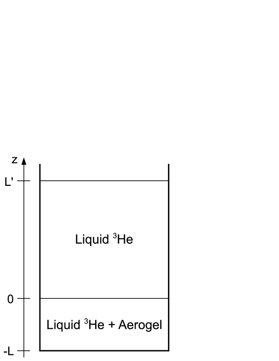
Figure 1: DN/TS system consisting of liquid ³He and aerogel. Liquid ³He in a container occupies $-L<z<L^{\prime}$ in which the aerogel is embedded in $-L<z<0$. When liquid ³He in the aerogel layer is in the normal state owing to impurity effect and the pure liquid ³He layer is in a superfluid state, this system is an ideal example of DN/TS junctions.

In this paper, we discuss the proximity effect in a DN/TS system consisting of superfluid ³He and the aerogel, as depicted in Fig. 1. Superfluid ³He is partly filled with the aerogel, which is used to introduce short-range impurity potentials in liquid ³He. A measure of the impurity effect is a ratio $\xi_{0}/l$, where $\xi_{0}$ is the coherence length and $l$ is the quasiparticle mean free path. A geometrical considerationThuneberg et al. (1998) for a typical aerogel with 98 % porosity leads to $l\sim$ 150 nm, which is comparable to $\xi_{0}$ of superfluid ³He and therefore a strong impurity effect is expected. One of the remarkable characteristics of this system is that the impurity effect can be controlled by pressure $P$: the coherence length $\xi_{0}$ increases with decreasing pressure, so that the system is relatively dirty at lower pressures. As a consequence, there exists a critical pressure $P_{c}$ below which the impurity effect is so strong that superfluid transition does not occur down to zero temperature.Matsumoto et al. (1997); Rainer and Sauls (1998); Higashitani (1999)

One can estimate $P_{c}$ from Green’s function theory for anisotropic pairing states with randomly distributed impurities.Rainer and Sauls (1998); Higashitani (1999) The theory predicts that the corresponding critical value of the ratio $\xi_{0}/l$ is $e^{-\gamma}/2\simeq 0.28$, where $\gamma=0.577\cdots$ is Euler’s constant and the coherence length $\xi_{0}$ is defined by $\xi_{0}=\hbar v_{F}/2\pi k_{B}T_{c0}$ with $v_{F}$ the Fermi velocity and $T_{c0}$ the critical temperature of pure liquid ³He. Putting $l=150$ nm gives a rough estimate, $P_{c}\simeq$ 5 bar (at which $\xi_{0}=42$ nm), in reasonable agreement with torsional oscillator experiments.Matsumoto et al. (1997) The system as in Fig. 1 below $P_{c}$ is an ideal example of DN/TS junctions. Moreover, at high pressures above $P_{c}$, one can study junctions with spin-triplet superfluids (TS’/TS system).

The purpose of this paper is to clarify the microscopic picture of the proximity effect in the dirty normal Fermi liquid/superfluid ³He system. A similar problem has been discussed by Kurki and ThunebergKurki and Thuneberg (2007) who calculated the self-consistent $p$-wave order parameter near the interface using the Ginzburg-Landau equation. A theory applicable to low temperatures was proposed by Tanaka et al.Tanaka et al. (2005b); Tanaka et al. (2004) They derived the boundary condition for the Usadel equationUsadel (1970) at the interface between the dirty normal metal and a clean unconventional superconductor. The Usadel equation treats isotropic superfluidity realized in dirty systems where non-$s$-wave pair functions are expected to be suppressed by impurity scattering. Near the interface, however, any partial wave components of the pair function can in general coexist. The Usadel equation cannot give information about such an interface effect on a microscopic scale. In this paper, we give detailed numerical results for the spatial dependence of the pair functions, obtained from the quasiclassical Green’s function theory valid for the whole temperature range and for arbitrary values of the mean free path. We also discuss the local density of states in the dirty normal layer.

This paper is organized as follows. In Sec. II, we describe the theoretical model and the quasiclassical theory. In Sec. III, we present the numerical results for the self-consistent $p$-wave order parameter, some partial wave components of the pair function, and the local density of states. Both of the weak scattering limit (Born approximation) and the strong one (unitarity limit) are considered for the impurity effect. The final section is devoted to conclusions. In the rest of this paper, we use the units $\hbar=k_{B}=1$.

II Formulation

We consider a dirty Fermi liquid/spin-triplet $p$-wave superfluid junction as depicted in Fig. 1. Liquid ³He in a container occupies $-L<z<L^{\prime}$ in which a region $-L<z<0$ is filled with aerogel. The container wall at $z=-L$ is simulated by a specular surface. The system is assumed to have translational symmetry in the $x$ and $y$ directions (this implies that the random average is taken over impurity positions). The width $L^{\prime}$ of the pure liquid ³He layer is assumed to be much longer than the coherence length $\xi_{0}$ and we put $L^{\prime}\rightarrow\infty$.

Let us discuss the quasiclassical Green’s function in the above system. Because of the translational symmetry in the $x$ and $y$ directions, one has only to consider one dimensional problem in the $z$ direction at a given parallel momentum component $(p_{x},p_{y})$. There exist two Fermi momenta when the parallel momentum is fixed, namely, $(p_{x},p_{y},+|p_{Fz}|)$ and $(p_{x},p_{y},-|p_{Fz}|)$, where $p_{Fz}$ is the $z$ component of the Fermi momentum. Then, the quasiclassical Green’s function can be specified by three variables: the coordinate $z$, the directional index $\alpha={\rm sign}(p_{Fz})$, and the complex energy variable $\epsilon$.

The quasiclassical Green’s function, which we denote by $\hat{g}_{\alpha}(\epsilon,z)$, obeysSerene and Rainer (1983)

$$\partial_{z}\hat{g}_{\alpha}(\epsilon,z)=[\hat{h}_{\alpha}(\epsilon,z),\ \hat{g}_{\alpha}(\epsilon,z)]$$ (1)

with

$$\hat{h}_{\alpha}(\epsilon,z)=\frac{\alpha i}{v_{Fz}}\left[\begin{pmatrix}\epsilon&\Delta_{\alpha}(z)\\ -\Delta_{\alpha}^{\dagger}(z)&-\epsilon\\ \end{pmatrix}-\hat{\sigma}^{\rm imp}(\epsilon,z)\right],$$ (2)

where $v_{Fz}$ is the $z$ component of the Fermi velocity, $\Delta_{\alpha}$ is the $2\times 2$ matrix of the $p$-wave order parameter, and $\hat{\sigma}^{\rm imp}$ is the impurity self-energy. The quasiclassical Green’s function $\hat{g}_{\alpha}$ is normalized as $\hat{g}^{2}_{\alpha}=-1$.

We assume superfluid ³He to be in the B phase. In this case, the order parameter can be expressed as

$$\Delta_{\alpha}(z)=\begin{pmatrix}-\Delta_{0}(z)\sin\theta\,e^{-i\phi}&\alpha\Delta_{1}(z)\cos\theta\\ \alpha\Delta_{1}(z)\cos\theta&\Delta_{0}(z)\sin\theta\,e^{i\phi}\\ \end{pmatrix},$$ (3)

where $\theta$ and $\phi$ are the polar and azimuthal angles, respectively. Note that in our notation the sign of $p_{Fz}=p_{F}\cos\theta$ is specified by $\alpha$ and therefore the polar angle $\theta$ is in the range $0<\theta<\pi/2$. For $z\rightarrow\infty$, the spatially dependent order parameters $\Delta_{0}(z)$ and $\Delta_{1}(z)$ tend to the same constant value, $\Delta_{B}$, corresponding to the energy gap in the bulk B phase (we take $\Delta_{B}$ to be real).

We describe the impurity effect within the self-consistent $t$-matrix approximationBuchholtz and Zwicknagl (1981); Higashitani (1999); Higashitani et al. (2005) for randomly distributed delta-function potentials. This formulation allows one to discuss both of the weak scattering regime (Born approximation) and the strong one (unitarity limit). In the two limits, the impurity self-energies are given by

$$\hat{\sigma}^{\rm imp}=\begin{cases}\displaystyle-\frac{1}{2\tau}\hat{G}&\mbox{(Born limit)}\\ \\ \displaystyle\frac{1}{2\tau}\hat{G}^{-1}&\mbox{(Unitarity limit)}\\ \end{cases}$$ (4)

with

$$\hat{G}=\frac{1}{2}\sum_{\alpha=\pm}\langle\hat{g}_{\alpha}\rangle$$ (5)

and $\tau=l/v_{F}$ the mean free time. Here,

$$\langle\cdots\rangle=\int_{0}^{\pi/2}\sin\theta\,d\theta\int_{0}^{2\pi}\frac{d\phi}{2\pi}\,(\cdots).$$ (6)

In the system under consideration, the impurity scattering rate $1/\tau$ changes discontinuously at the interface: it is zero in the region of pure superfluid ³He ($z>0$) and finite otherwise ($-L<z<0$).

Equation (1) is supplemented by the following boundary conditions. In the asymptotic region ($z\rightarrow\infty$), the quasiclassical Green’s function takes the bulk form

$$\hat{g}_{\alpha}(\epsilon,z)\xrightarrow{z\rightarrow\infty}\frac{1}{\sqrt{\Delta_{B}^{2}-\epsilon^{2}}}\begin{pmatrix}\epsilon&\Delta_{\alpha}(\infty)\\ -\Delta_{\alpha}^{\dagger}(\infty)&-\epsilon\\ \end{pmatrix}.$$ (7)

At the interface ($z=0$), $\hat{g}_{\alpha}$ is continuously connected. At the wall ($z=-L$), it satisfies the specular surface boundary condition

$$\hat{g}_{+}(\epsilon,-L)=\hat{g}_{-}(\epsilon,-L).$$ (8)

The above set of equations enables one to determine the quasiclassical Green’s function $\hat{g}_{\alpha}$ in the present system. As shown by Nagato et al.Nagato et al. (1993, 1996) and Higashitani and Nagai,Higashitani and Nagai (1995) the calculation of $\hat{g}_{\alpha}$ can be reduced to solving simple and numerically stable differential equations of the Riccati type. They treated the cases of $2\times 2$ matrix Green’s functions. A similar problem for $4\times 4$ matrix cases was discussed by Eschrig.Eschrig (2000) Following them, we write $\hat{g}_{\alpha}$ as

$$\hat{g}_{\alpha}=\begin{pmatrix}[1+{\cal D}_{\alpha}\tilde{\cal D}_{\alpha}]^{-1}&0\\ 0&[1+\tilde{\cal D}_{\alpha}{\cal D}_{\alpha}]^{-1}\\ \end{pmatrix}\begin{pmatrix}i[1-{\cal D}_{\alpha}\tilde{\cal D}_{\alpha}]&2{\cal D}_{\alpha}\\ -2\tilde{\cal D}_{\alpha}&-i[1-\tilde{\cal D}_{\alpha}{\cal D}_{\alpha}]\\ \end{pmatrix}$$ (9)

in which ${\cal D}_{\alpha}$ and $\tilde{\cal D}_{\alpha}$ are $2\times 2$ matrices obeying the Riccati type differential equations

$$\alpha v_{Fz}\partial_{z}{\cal D}_{\alpha}=i(a_{\alpha}{\cal D}_{\alpha}+{\cal D}_{\alpha}\tilde{a}_{\alpha})+b_{\alpha}-{\cal D}_{\alpha}\tilde{b}_{\alpha}{\cal D}_{\alpha},$$ (10)

$$\alpha v_{Fz}\partial_{z}\tilde{\cal D}_{\alpha}=-i(\tilde{a}_{\alpha}\tilde{\cal D}_{\alpha}+\tilde{\cal D}_{\alpha}a_{\alpha})-\tilde{b}_{\alpha}+\tilde{\cal D}_{\alpha}{b}_{\alpha}\tilde{\cal D}_{\alpha}.$$ (11)

Here, we have put

$$\hat{h}_{\alpha}=\frac{\alpha i}{v_{Fz}}\begin{pmatrix}a_{\alpha}&b_{\alpha}\\ -\tilde{b}_{\alpha}&-\tilde{a}_{\alpha}\\ \end{pmatrix}.$$ (12)

We can further simplify the calculation by taking into account the matrix structure of the order parameter in the B phase. One can write $\Delta_{\alpha}$ as

$$\Delta_{\alpha}=V\sigma_{1}[(\alpha\Delta_{\perp}+i\Delta_{\parallel})\sigma_{+}+(\alpha\Delta_{\perp}-i\Delta_{\parallel})\sigma_{-}]V,$$ (13)

where

$$\Delta_{\parallel}=\Delta_{0}\sin\theta,$$ (14)

$$\Delta_{\perp}=\Delta_{1}\cos\theta,$$ (15)

$$V=\exp\left(-\frac{i}{2}\phi\,\sigma_{3}\right),$$ (16)

$$\sigma_{\pm}=\frac{1}{2}(1\pm\sigma_{2}),$$ (17)

and $\sigma_{i}$’s ($i=1,2,3$) are the Pauli matrices. Note that $\sigma_{\pm}$ are projection operators satisfying

$$\sigma_{\pm}^{2}=\sigma_{\pm},\quad\sigma_{+}\sigma_{-}=\sigma_{-}\sigma_{+}=0,\quad\sigma_{+}+\sigma_{-}=1.$$ (18)

Equation (13) suggests the following parameterization:

$${\cal D}_{\alpha}=V\sigma_{1}({\cal F}_{\alpha}\sigma_{+}+\tilde{\cal F}_{\alpha}\sigma_{-})V,$$ (19)

$$\tilde{\cal D}_{\alpha}=-V^{\dagger}({\cal F}_{-\alpha}\sigma_{+}+\tilde{\cal F}_{-\alpha}\sigma_{-})\sigma_{1}V^{\dagger},$$ (20)

where ${\cal F}_{\alpha}$ and $\tilde{\cal F}_{\alpha}$ are scalar functions. Using Eqs. (19) and (20), the angle-averaged Green’s function $\hat{G}$ is found to have the form

$$\hat{G}=\begin{pmatrix}iG&F\sigma_{1}\\ F\sigma_{1}&-iG\\ \end{pmatrix}$$ (21)

with

$$G=\frac{1}{2}\left\langle\frac{1+\lambda}{1-\lambda}+\frac{1+\tilde{\lambda}}{1-\tilde{\lambda}}\right\rangle,$$ (22)

$$F=\frac{1}{2}\left\langle\frac{{\cal F}_{+}+{\cal F}_{-}}{1-\lambda}+\frac{\tilde{\cal F}_{+}+\tilde{\cal F}_{-}}{1-\tilde{\lambda}}\right\rangle,$$ (23)

where $\lambda={\cal F}_{+}{\cal F}_{-}$ and $\tilde{\lambda}=\tilde{\cal F}_{+}\tilde{\cal F}_{-}$. The function ${\cal F}_{\alpha}$ obeys

$$\alpha v_{Fz}\partial_{z}{\cal F}_{\alpha}=2ih{\cal F}_{\alpha}+f_{\alpha}+f_{-\alpha}{\cal F}_{\alpha}^{2},$$ (24)

where

$$h=\epsilon+\frac{i}{2\tau}G,$$ (25)

$${f}_{\alpha}=\alpha\Delta_{\perp}+i\Delta_{\parallel}+\frac{1}{2\tau}F.$$ (26)

The boundary conditions are

• $z\rightarrow\infty$: $\displaystyle{{\cal F}_{-}=\lim_{z\rightarrow\infty}\frac{if_{-}}{h+i\sqrt{-f_{+}f_{-}-h^{2}}}}$.

• $z=0$: ${\cal F}_{\alpha}$ is continuous.

• $z=-L$: ${\cal F}_{+}={\cal F}_{-}$.

The function $\tilde{\cal F}_{\alpha}$ obeys the same set of equations as ${\cal F}_{\alpha}$ but with $\Delta_{\parallel}$ replaced by $-\Delta_{\parallel}$. Thus, the $4\times 4$ matrix equation for $\hat{g}_{\alpha}$ is reduced to the four scalar ones for ${\cal F}_{\pm}$ and $\tilde{\cal F}_{\pm}$.

It is useful to note that ${\cal F}_{\alpha}(\epsilon,z)$ and $\tilde{\cal F}_{\alpha}(\epsilon,z)$ on the imaginary axis ($\epsilon=iE$) of the complex $\epsilon$ plane satisfy the symmetry relation

$${\cal F}_{\alpha}^{*}(iE,z)=\tilde{\cal F}_{\alpha}(iE,z),$$ (27)

$${\cal F}_{\alpha}(-iE,z)=1/\tilde{\cal F}_{\alpha}(iE,z).$$ (28)

Equation (27) allows one to construct the Matsubara Green’s function only from ${\cal F}_{\alpha}$. It follows also from Eq. (27) that the angle averaged Green’s functions $G$ and $F$ at $\epsilon=iE$ are real quantities [see Eqs. (22) and (23)]. Equation (28) is associated with the parity of Green’s function in the Matsubara frequency $\epsilon=i\epsilon_{n}=i\pi T(2n+1)$. For example, one can show that the spin-triplet $s$-wave pair function $F$ is odd in $\epsilon_{n}$, as expected.

Finally we discuss briefly how we can treat the case when the B-phase order parameter in the asymptotic region takes a more general form $\Delta_{\alpha}(z\rightarrow\infty)=\Delta_{B}R_{\mu j}({\bf n},\vartheta)\hat{p}_{j}\sigma_{\mu}i\sigma_{2}$, where $\hat{p}_{j}=p_{j}/p_{F}$ and $R_{\mu j}({\bf n},\vartheta)$ is a rotation matrix around an axis ${\bf n}$ by an angle $\vartheta$. Our analysis of the quasiclassical Green’s function relies on a particular choice of the order parameter [see Eq. (3)], corresponding to $R_{\mu j}=\delta_{\mu j}$. It is easy to generalize our formulation to the case of arbitrary $R_{\mu j}$. Since $R_{\mu j}\sigma_{\mu}=U\sigma_{j}U^{\dagger}$ with $U=\exp(-i\bm{\sigma}\cdot{\bf n}\vartheta/2)$, the quasiclassical Green’s function for arbitrary $R_{\mu j}$ can be obtained from the one for $R_{\mu j}=\delta_{\mu j}$ by a spin-space rotation described by $U$. This means that the difference between the quasiclassical Green’s functions for different choice of $R_{\mu j}$ is only the matrix structure in spin space. For example, the (1,2)-component (in particle-hole space) of the angle-averaged Green’s function $\hat{G}$ for $R_{\mu j}=\delta_{\mu j}$ has the form $F\sigma_{1}=F\sigma_{3}i\sigma_{2}$ [see Eq. (21)] and is transformed by the rotation to $FU\sigma_{3}U^{\dagger}i\sigma_{2}=FR_{\mu 3}\sigma_{\mu}i\sigma_{2}$. In the present study of the proximity effect such a difference in the spin structure is not important and all the numerical results presented below are the same regardless of the choice of $R_{\mu j}$.

III Numerical results

In this section, we show some numerical results relevant to the proximity effect. We discuss, in separate subsections, the self-consistent $p$-wave order parameter, the odd-frequency $s$-wave pair function, non-$s$-wave pair functions, and the local density of states. The numerical results given there are those obtained within the Born approximation. The effect of the strong scattering shall be discussed in the final subsection. All the numerical calculations are performed at a temperature $T=0.2T_{c0}$ ($T_{c0}$ is the critical temperature of pure liquid ³He), which is low enough for the $p$-wave order parameter in the bulk superfluid ³He to be well developed.

III.1 Self-consistent $p$-wave order parameter

The $p$-wave order parameter must be determined self-consistently from the gap equation with the pairing interaction $v_{\hat{p},\hat{p}^{\prime}}=-3g_{1}{\hat{p}}\cdot{\hat{p}}^{\prime}$, where ${\hat{p}}$ is the unit vector specifying the direction of the Fermi momentum. The gap equation can be written in terms of ${\cal F}_{\alpha}$ as

$$\frac{\Delta_{0}(z)}{g_{1}N(0)}=3\pi T\sum_{\epsilon_{n}>0}^{\epsilon_{c}}\left\langle\sin\theta\,{\rm Im}\,A^{+}(i\epsilon_{n},z)\right\rangle,$$ (29)

$$\frac{\Delta_{1}(z)}{g_{1}N(0)}=6\pi T\sum_{\epsilon_{n}>0}^{\epsilon_{c}}\left\langle\cos\theta\,{\rm Re}\,A^{-}(i\epsilon_{n},z)\right\rangle,$$ (30)

$$A^{\pm}(i\epsilon_{n},z)=\frac{{\cal F}_{+}(i\epsilon_{n},z)\pm{\cal F}_{-}(i\epsilon_{n},z)}{1-\lambda(i\epsilon_{n},z)},$$ (31)

where $N(0)$ is the density of states at the Fermi level and $\epsilon_{c}$ is a cutoff energy.

We have calculated the self-consistent order parameter by solving the above equations iteratively. In the numerical calculations, the coupling constant is evaluated fromKieselmann (1987)

$$\frac{1}{g_{1}N(0)}=\ln\frac{T}{T_{c0}}+2\pi T\sum_{\epsilon_{n}>0}^{\epsilon_{c}}\frac{1}{\epsilon_{n}}$$ (32)

and the Matsubara summation is cut off at $\epsilon_{c}=10\pi T_{c0}$.

Typical results of the spatial dependence of $\Delta_{0}(z)$ and $\Delta_{1}(z)$ are shown in Fig. 2. We take the width $L$ of the aerogel layer to be $20\xi_{0}$. The impurity effect by the aerogel is characterized by the parameter $\xi_{0}/l$ and is evaluated within the Born approximation. Numerical results for two cases with $\xi_{0}/l=0.1,0.5$ are shown. When $l=150$ nm (see Sec. I), the parameters $\xi_{0}/l=0.1$ and $\xi_{0}/l=0.5$ correspond to pressures $\sim 34$ bar (above the critical pressure $P_{c}$) and $\sim 0$ bar (below $P_{c}$), respectively.

For $\xi_{0}/l=0.5$, the impurity effect is strong enough to destroy bulk $p$-wave superfluidity of ³He. In this case, the $p$-wave order parameters in the aerogel layer exhibit exponential decay typical for the proximity effect.

In the relatively clean case with $\xi_{0}/l=0.1$, the $p$-wave order parameters survive even in the region far from the interface. Thus, the surface effect characteristic of the B phase is expected near the wall (at $z/\xi_{0}=-20$).Buchholtz and Zwicknagl (1981); Nagato et al. (1998) The strong suppression of $\Delta_{1}$ and the enhancement of $\Delta_{0}$ near the wall are due to the surface effect. Near the interface, on the other hand, both of $\Delta_{0}$ and $\Delta_{1}$ are suppressed by the impurity effect.

III.2 Odd-frequency $s$-wave pair function

In this subsection, we discuss the odd-frequency spin-triplet $s$-wave pair corresponding to the function $F$ [see Eqs. (21) and (23)]. Here, we are interested in $F$ in the normal liquid ³He-aerogel layer.

First of all, we mention a qualitative picture expected from the dirty-limit theory. The DN layer is characterized by three parameters: the diffusion constant $D=v_{F}l/3$, the Matsubara frequency $\epsilon_{n}$, and the layer width $L$, as can be seen from the Usadel equation.Usadel (1970) From dimensional analysis, we have a characteristic length scale $\xi_{d}(\epsilon_{n})=\sqrt{D/\epsilon_{n}}$ and a characteristic energy scale $E_{\rm Th}=D/L^{2}$ (the Thouless energy). The length $\xi_{d}(\epsilon_{n})$ is essentially equivalent to the temperature-dependent coherence length $\xi_{N}=\sqrt{D/2\pi T}$ in the DN layer. As has been shown in the study of the proximity effect in metals,deGennes ; Deutscher $\xi_{N}$ gives the length scale of the exponential decay of the proximity-induced pair function in the dirty limit. The frequency-dependent coherence length $\xi_{d}(\epsilon_{n})$ characterizes the spatial variation of $F$ in the dirty limit. At high frequencies $\epsilon_{n}\gg E_{\rm Th}$, $\xi_{d}(\epsilon_{n})$ is much shorter than $L$. This means that $F$ is exponentially small near the layer end. On the other hand, at low frequencies $\epsilon_{n}\ll E_{\rm Th}$, $F$ extends over the whole layer. For $\epsilon_{n}\rightarrow 0$, in particular, $\xi_{d}(\epsilon_{n})$ diverges, so that a long range proximity effect is expected.

In Fig. 3, our numerical results for $F(\epsilon,z)$ are shown for various values of imaginary frequencies ($\epsilon=iE$) scaled by $E_{\rm Th}$. The impurity effect is evaluated at $\xi_{0}/l=0.5$ in the Born limit. The numerical results support the above qualitative picture. At a high frequency $E/E_{\rm Th}=100$, $F$ is localized near the interface. With decreasing frequency, the penetration distance of $F$ increases. The magnitude of $F$ also increases with decreasing frequency.

We note here that the odd-frequency $s$-wave pair function $F$ does not appear when the superfluid layer ($z>0$) does not have the perpendicular component $\Delta_{\perp}$ of the $p$-wave order parameter. This can be analytically shown in the following way. Putting $\Delta_{\perp}=0$ and assuming that $F=0$, one can readily find a relation $\tilde{\cal F}_{\alpha}=-{\cal F}_{\alpha}$. Then, the upper-right $2\times 2$ submatrix of $\hat{g}_{\alpha}$ (which we denote by $\hat{g}^{12}_{\alpha}$) takes the form

$$\hat{g}_{\alpha}^{12}=\frac{2i{\cal F}_{\alpha}}{1-\lambda}\begin{pmatrix}e^{-i\phi}&0\\ 0&-e^{i\phi}\\ \end{pmatrix}.$$ (33)

This form of $\hat{g}_{\alpha}^{12}$ is consistent with the assumption of $F=0$. Thus, when $\Delta_{\perp}=0$, the pair function has only the $p$-wave components parallel to the interface.

III.3 Proximity effect of non-$s$-wave pair functions

There can coexist any partial wave components of the pair function near the interface that breaks translational symmetry. Here, we give numerical results of the spatial dependence of the $p$-wave and $d$-wave components.

The $p$-wave components have even-frequency spin-triplet symmetry and summing them up over the Matsubara frequencies gives the $p$-wave order parameter. One can define three $p$-wave components $F_{1}^{x,y,z}$ as

$$\frac{1}{2}\sum_{\alpha=\pm}\left\langle\hat{p}_{x}\,\hat{g}_{\alpha}^{12}\right\rangle=F_{1}^{x}\sigma_{1}i\sigma_{2},$$ (34)

$$\frac{1}{2}\sum_{\alpha=\pm}\left\langle\hat{p}_{y}\,\hat{g}_{\alpha}^{12}\right\rangle=F_{1}^{y}\sigma_{2}i\sigma_{2},$$ (35)

$$\frac{1}{2}\sum_{\alpha=\pm}\left\langle\alpha\hat{p}_{z}\,\hat{g}_{\alpha}^{12}\right\rangle=F_{1}^{z}\sigma_{3}i\sigma_{2}.$$ (36)

It is obvious from the symmetry of the system that

$$F_{1}^{x}=F_{1}^{y}.$$ (37)

The $d$-wave components are odd-frequency spin-triplet pairs, as well as the $s$-wave one. As an example of the $d$-wave components, we consider

$$\frac{1}{2}\sum_{\alpha=\pm}\left\langle\frac{1}{2}(3\hat{p}_{z}^{2}-1)\hat{g}_{\alpha}^{12}\right\rangle=F_{2}\sigma_{3}i\sigma_{2}.$$ (38)

In Fig. 4, we show the spatial dependence of the $p$-wave and $d$-wave pair functions for $\xi_{0}/l=0.5$ in the Born limit. The corresponding result for the $s$-wave pair function is also shown for comparison. All the components coexist around the interface. In the DN layer except near the interface, the non-$s$-wave components are much smaller than the $s$-wave one and the proximity-induced superfluidity is dominated by the odd-frequency $s$-wave pair.

III.4 Local density of states

We now discuss the local density of states (LDOS),

$$n(\epsilon,z)={\rm Re}\,G(\epsilon+i0,z).$$ (39)

Figure 5 shows LDOS in the Born limit with $\xi_{0}/l=0.5$. LDOS at the interface (dotted line) has a peak at $\epsilon/\Delta_{B}=1$ above which it decreases with increasing $\epsilon$ and tends to unity (corresponding to the normal-state value) for $\epsilon\rightarrow\infty$. The finite LDOS at low energies $\epsilon/\Delta_{B}<1$ is due to the existence of bound states decaying into the pure superfluid layer. At the layer end (solid line), on the other hand, LDOS has a sharp peak at zero energy and is unity in almost all the other energies. At a position near the interface (dashed line), LDOS shows an intermediate behavior between the two cases.

The width of the zero-energy peak in LDOS at the layer end is of order the Thouless energy $E_{\rm Th}$. In the present system, $E_{\rm Th}$ is much smaller than $\Delta_{B}$ ($E_{\rm Th}/\Delta_{B}\sim 6\times 10^{-3}$). The peak structure around $\epsilon=0$ is magnified in Fig. 6. Here, we plot LDOS at $z/L=-1,-3/4,-1/2$ as a function of $\epsilon/E_{\rm Th}$. It is, at first glance, surprising that a sizable peak appears in LDOS near the layer end where the $p$-wave order parameter almost vanishes [see Fig. 2(a)]. It should be noted, however, that at low energies below $\epsilon\sim E_{\rm Th}$ the $s$-wave pair function has a finite amplitude even near the layer end though non-$s$-wave pair functions are vanishingly small there (see Fig. 4). The zero-energy peak structure below $\epsilon\sim E_{\rm Th}$ in LDOS in the DN layer is due to the existence of the odd-frequency $s$-wave pair.

III.5 Effect of strong impurity scattering

All the above numerical results are calculated within the Born approximation. Here, we discuss the strong scattering effect as described by the impurity self-energy in the unitarity limit.

As is well known, the impurity effect in anisotropic superfluid states is quite different between the weak and strong scattering regimes. In our theory such a difference originates from the anisotropy (momentum dependence) of the quasiclassical Green’s function $\hat{g}_{\alpha}$. Note that, when $\hat{g}_{\alpha}$ is isotropic, the angle average of $\hat{g}_{\alpha}$, namely, $\hat{G}$ has a property $\hat{G}^{2}=-1$ similar to the normalization condition $\hat{g}_{\alpha}^{2}=-1$. Then, the impurity self-energy in the unitarity limit has the same form as that in the Born limit [see Eq. (4)].

The above observation implies that the impurity effects in the DN layer are insensitive to scattering regime because of isotropization by impurity scattering. To demonstrate that, we plot in Fig. 7 the matrix elements $G$ and $F$ of $\hat{G}$ for $\xi_{0}/l=0.5$ as a function of $z/\xi_{0}$ in both of the Born and unitarity limits. The difference between the two scattering limits is quite small and $\hat{G}^{2}=F^{2}-G^{2}=-1$ is well satisfied in the DN layer except near the interface. We have compared the other Born-limit numerical results presented previous subsections for $\xi_{0}/l=0.5$ with the corresponding results in the unitarity limit and found also no significant difference.

On the other hand, when $\xi_{0}/l$ is sufficiently small and liquid ³He in the aerogel is in the $p$-wave superfluid state, substantial differences can occur. As an example, we show in Fig. 8 the spatial dependence of the $p$-wave order parameter. The unitarity-limit scattering gives rise to stronger pair-breaking. This effect is clearly seen for $\xi_{0}/l=0.1$ but is quite small for $\xi_{0}/l=0.5$.

IV Conclusions

Using the quasiclassical Green’s function theory, we have discussed the proximity effect in the liquid ³He-aerogel composite in contact with bulk superfluid ³He-B. This system is an ideal model system for studying the proximity effect in dirty normal Fermi liquid/spin-triplet superfluid junctions when the impurity pair-breaking effect by the aerogel is strong enough to destroy the superfluidity of liquid ³He. Such a situation occurs at low pressures below the critical pressureMatsumoto et al. (1997); Rainer and Sauls (1998); Higashitani (1999) or at temperatures higher than the reduced critical temperature of liquid ³He in the aerogel. We have proposed a convenient Green’s function parameterization that reduces the $4\times 4$ matrix equation for superfluid ³He-B to four scalar differential equations of the Riccati type. We used this method to calculate self-consistently the spatial variations of the $p$-wave order parameter and the impurity self-energy. To clarify the microscopic structure of the proximity-induced superfluidity, we have analyzed in detail the frequency and momentum dependent pair function and the local density of states in the aerogel layer.

Although the order parameter in the above system is purely $p$-wave, any partial wave components of the pair function can coexist owing to broken translational symmetry. We have shown that such an admixture of the Cooper pairs, in fact, occurs around the aerogel/superfluid ³He-B interface. Among those, only the $s$-wave pair can penetrate deep into the aerogel layer. This is because non-$s$-wave pairs are destroyed by impurity scattering in the interior of the aerogel layer. As is expected qualitatively from the Usadel equation and was confirmed by our fully self-consistent numerical calculations, the $s$-wave pair function extends over the whole aerogel layer when the frequency is of order or less than the Thouless energy $E_{\rm Th}$. The $s$-wave pair in the present system has odd-frequency symmetry and therefore the proximity-induced superfluidity in a thick aerogel layer is an example of the odd-frequency pairing states.

We have found that the local density of states in the aerogel layer has a zero-energy peak of width of order $E_{\rm Th}$, in agreement with previous theoretical worksTanaka and Kashiwaya (2004); Tanaka et al. (2005a, b); Tanaka and Golubov (2007) using the Usadel equation. The aerogel layer considered here has such a thick width that the $p$-wave order parameter almost vanishes near the layer end. Nonetheless, a sizable zero-energy peak appears in the local density of states near the layer end. This is a manifestation of the long range proximity effect of the $s$-wave pair function at frequencies below $\epsilon\sim E_{\rm Th}$.

One of the remaining problems which we have not addressed in the present paper is what characteristics in observables arise from the odd-frequency $s$-wave paring. Further studies in this direction are in progress.

Figure 2: Spatial variation of the self-consistent $p$-wave order parameter in the Born limit with (a) $\xi_{0}/l=0.5$ and (b) $\xi_{0}/l=0.1$. The vertical axis is $\Delta_{0,1}$ scaled by the bulk gap $\Delta_{B}$ of superfluid ³He-B. The ³He-aerogel layer occupies $-20<z/\xi_{0}<0$ and is in contact with bulk superfluid ³He-B at $z=0$. In the aerogel layer far from the interface, impurity scattering destroys the $p$-wave Cooper pair for $\xi_{0}/l=0.5$, but does not for $\xi_{0}/l=0.1$.

Figure 3: Spatial dependence of the odd-frequency spin-triplet $s$-wave pair function $F(iE,z)$ at various values of $E/E_{\rm Th}$ in the same DN/TS system as in Fig. 2(a).

Figure 4: Spatial dependence of some partial wave components of the pair function at an imaginary frequency $\epsilon=iE$ with $E/E_{\rm Th}=0.5$ in the same DN/TS system as in Fig. 2(a).

Figure 5: LDOS in the same DN/TS system as in Fig. 2(a). Three lines are those at the DN layer end (solid line), at the interface (dotted line), and at $z=z^{*}$ (dashed line), a position near the interface in the DN layer, so defined that $\Delta_{1}(z^{*})/\Delta_{1}(0)=1/2$.

Figure 6: LDOS as a function of $\epsilon/E_{\rm Th}$. Numerical results at three positions $z/L=-1,-3/4,-1/2$ in the DN layer are shown for the same DN/TS system as in Fig. 2(a).

Figure 7: Comparison between the Born-limit (solid lines) and the unitarity-limit (dotted lines) results for the spatial dependence of the matrix elements $G$ and $F$ of the angle averaged Green’s function $\hat{G}(iE,z)$ at $E/E_{\rm Th}=1$ for $\xi_{0}/l=0.5$. The results for $G$ and $F$ in the unitarity limit are almost the same as those in the Born limit. The spatial dependence of $\hat{G}^{2}=F^{2}-G^{2}$ in the Born limit is plotted for reference (see text).

Figure 8: Comparison between the Born-limit (solid lines) and the unitarity-limit (dotted lines) results for the spatial dependence of the self-consistent $p$-wave order parameter. The numerical data in the Born limit are the same as those in Fig. 2. For $\xi_{0}/l=0.5$, the results in the two limits are almost the same.