Dynamical mean-field theory and numerical renormalization group study of superconductivity in the attractive Hubbard model

Abstract

We present a study of the attractive Hubbard model based on the dynamical mean field theory (DMFT) combined with the numerical renormalization group (NRG). For this study the NRG method is extended to deal with self-consistent solutions of effective impurity models with superconducting symmetry breaking. We give details of this extension and validate our calculations with DMFT results with antiferromagnetic ordering. We also present results for static and integrated quantities for different filling factors in the crossover from weak (BCS) to strong coupling (BEC) superfluidity. We study the evolution of the single-particle spectra throughout the crossover regime. Although the DMFT does not include the interaction of the fermions with the Goldstone mode, we find strong deviations from the mean-field theory in the intermediate and strong coupling (BEC) regimes. In particular, we show that low-energy charge fluctuations induce a transfer of spectral weight from the Bogoliubov quasiparticles to a higher-energy incoherent hump.

I Introduction

The Hubbard model of locally interacting fermions plays a fundamental role in the theory of condensed matter physics and has become a standard model to study correlated electronic behavior. In its repulsive version depending on interaction strength and doping it displays magnetic instabilities such as antiferromagnetism. However, there is also evidence Halboth and Metzner (2000); Zanchi and Schulz (2000); Honerkamp et al. (2001); Aichhorn et al. (2006) that there is a parameter range where it possesses a strong instability in the pairing channel to d-wave superconductivity, which makes it a good candidate to describe many important aspects of the high temperature superconductors. Its attractive counterpart, the model with an onsite pairing term, has a simpler phase diagram, as the ground state is an s-wave superconductor. At half filling a degenerate charge ordered state can also occur. For electrons in a solid this model may seem inappropriate at first sight, but one can think of the local attraction between the electrons as mediated by a boson, for instance, a phonon or exciton, where any form of retardation is neglected.Micnas et al. (1990) Indeed, the Bardeen, Cooper, and Schrieffer (1957) (BCS) theory for superconductivity uses a similar model with instantaneous local attraction albeit with an energy (Debye) cutoff. In ultracold atom experiments Bloch et al. (2008) the interactions between the fermionic atoms in an optical trap can be tuned by a Feshbach resonance. For a broad resonance there exists a regime where the effective interaction is well described by a local attraction. Superfluidity has been observed in such systems Greiner et al. (2003); Zwierlein et al. (2004, 2005); Bloch et al. (2008), also in the case where the fermions are confined to an optical lattice Chin et al. (2006).

When tuning the interaction in models of attractive fermions, such as the attractive Hubbard model, one has two limiting cases, that of weak coupling BCS superfluidity and the strong coupling Bose Einstein condensation (BEC) of preformed pairs. The theoretical understanding which has been developed over the years is that the properties, such as the order parameter $\Delta_{\rm sc}$ and the transition temperature $T_{c}$ to the superfluid state, are connected by a smooth crossover, and approximate interpolation schemes between these limits have been devised Eagles (1969); Leggett (1980); Nozières and Schmitt-Rink (1985); Randeria (1995). Apart from its recent experimental realization for ultracold atoms in an optical trap Greiner et al. (2003); Zwierlein et al. (2004, 2005); Bloch et al. (2008), there is experimental evidence that this BCS-BEC crossover has also relevance for strong coupling and high temperature superconductors. It has been claimed that these superconductors display properties in certain parts of the phase diagram, such as the pseudo-gap, that can be understood in terms of pairs, preformed above the transition temperature $T_{c}$, in contrast to the BCS picture, where the pairs no longer exist above $T_{c}$.Micnas et al. (1990); Toschi et al. (2005a); Chen et al. (2006)

Many aspects of the attractive Hubbard model have already been investigatedMicnas et al. (1990); Dupuis (2004). However, the dynamic response functions have received fairly little theoretical attention, and it is the predictions for these quantities through the crossover that will be the focus of the present paper. One particular question concerns the fermionic excitations in the one particle spectral functions. These are dominated by sharp Bogoliubov excitations in the weak coupling limit. However, at strong coupling, when the fermions are bound to pairs, we expect a decrease of the spectral weight carried by the Bogoliubov quasiparticles. In order to investigate in detail what happens throughout the crossover a suitable approach to calculate dynamic quantities is required. In situations where the momentum dependence of the self-energy is not so important, such as in the Mott transition, the dynamical mean field theory (DMFT) has proven to be useful as local interactions can be treated very accurately. A variety of methods such as perturbation theory, quantum Monte Carlo, as well as exact diagonalization (ED) and numerical renormalization group (NRG) are commonly used to solve the effective impurity model. Amongst these methods the NRG is one of the more suitable ones to calculate low temperature spectral functions. Since it was originally proposed by Wilson Wilson (1975), it has been developed constantly over the years.Bulla et al. (2008) The way of calculating spectral functions has been given a solid basis by the recent approachPeters et al. (2006); Weichselbaum and von Delft (2007) based on complete basis set proposed by Anders and Schiller Anders and Schiller (2005). So far the NRG has, however, not been applied to self-consistent DMFT calculations with superconducting symmetry breaking. Here we will show in detail how the method can be extended to this situation and present results for the spectral functions. Some of the results have already been published in Ref. Bauer and Hewson, 2009. DMFT studies for the attractive Hubbard model based on other ’impurity solvers’ have been carried out in the normal phaseKeller et al. (2001); Capone et al. (2002), and in the broken symmetry phaseGarg et al. (2005); Toschi et al. (2005b, a). There is also a recent study in two dimensions with cellular DMFT Kyung et al. (2006).

Our paper is organized as follows. The model and DMFT-NRG approach are described in section II. For this calculation the DMFT-NRG approach has to be generalized to deal with the case of a superconducting bath. This generalization is described in detail in section III. There is a mapping from the negative $U$ model to the positive one when the lattice is bipartite. In the half filled case this mapping can be used to check the results for superconductivity with earlier DMFT-NRG calculations with antiferromagnetic order. The mapping and comparison of the results is given in section IV. In section V we compare our results for static and integrated quantities, such as the anomalous expectation value or superfluid density, with results based on other approximations. Finally in section VI we present results for dynamic response functions. We focus on the features in the one-electron spectral density. Dynamic susceptibilities calculated with the method described here have been reported in Ref. Bauer and Hewson, 2009.

II Model and DMFT-NRG setup

The subject of this paper is a study of the attractive Hubbard model, which in the grand canonical formalism reads

$$H=\sum_{i,j,\sigma}(t_{ij}c^{\dagger}_{i,\sigma}c_{j,\sigma}+\mathrm{h.c.})-\mu\sum_{i\sigma}n_{i\sigma}-U\sum_{i}n_{i,\uparrow}n_{i,\downarrow},$$ (1)

with the chemical potential $\mu$, the interaction strength $U>0$ and the hopping parameters $t_{ij}$. $c^{\dagger}_{i,\sigma}$ creates a fermion at site $i$ with spin $\sigma$, and $n_{i,\sigma}=c^{\dagger}_{i,\sigma}c_{i,\sigma}$. The present calculations are confined to zero temperature, however, an extension to finite temperature is possible. To study superconducting order we can include an explicit superconducting symmetry breaking term,

$$H_{\rm sc}=\Delta^{0}_{\rm sc}\sum_{{\bm{k}}}[c^{\dagger}_{{\bm{k}},\uparrow}c^{\dagger}_{-{\bm{k}},\downarrow}+\mathrm{h.c.}],$$ (2)

with an “external field” $\Delta_{\rm sc}^{0}$. In the superconducting case in Nambu space the Green’s function matrix is given by

$$\underline{G}_{{\bm{k}}}(\omega)=\left(\begin{array}[]{c c}\langle\!\langle c_{{\bm{k}},\uparrow};c^{\dagger}_{{\bm{k}},\uparrow}\rangle\!\rangle_{\omega}&\langle\!\langle c_{{\bm{k}},\uparrow};c_{-{\bm{k}},\downarrow}\rangle\!\rangle_{\omega}\\ \langle\!\langle c^{\dagger}_{-{\bm{k}},\downarrow};c^{\dagger}_{{\bm{k}},\uparrow}\rangle\!\rangle_{\omega}&\langle\!\langle c^{\dagger}_{-{\bm{k}},\downarrow};c_{-{\bm{k}},\downarrow}\rangle\!\rangle_{\omega}\end{array}\right),$$ (3)

where we use the notation for zero temperature retarded Green’s functions for two operators $A,B$, $\langle\!\langle A;B\rangle\!\rangle_{\omega}:=-i\!\int\limits\!\!{\rm d}t\;\theta(t)\mathrm{e}^{i\omega t}\langle[A(t),B]\ \!\!\rangle$ with the expectation value in the ground state $\langle\ldots\ \!\!\rangle$. Upon including (2) the non-interacting Green’s function matrix $\underline{G}_{{\bm{k}}}^{0}(\omega)$ has the form,

$$\underline{G}_{{\bm{k}}}^{0}(\omega)^{-1}=\left(\begin{array}[]{cc}\omega-\xi_{{\bm{k}}}&\Delta^{0}_{\rm sc}\\ \Delta^{0}_{\rm sc}&\omega+\xi_{{\bm{k}}}\end{array}\right),$$ (4)

where $\xi_{{\bm{k}}}=\varepsilon_{{\bm{k}}}-\mu$. For the interacting system we introduce the matrix self-energy $\underline{\Sigma}_{{\bm{k}}}(\omega)$ such that the inverse of the full Green’s function matrix $\underline{G}_{{\bm{k}}}(\omega)$ is given by the Dyson equation

$$\underline{G}_{{\bm{k}}}(\omega)^{-1}=\underline{G}_{{\bm{k}}}^{0}(\omega)^{-1}-\underline{\Sigma}_{{\bm{k}}}(\omega).$$ (5)

We employ the dynamical mean field theory to analyze the model (1). As effective impurity model we consider the attractive Anderson impurity model in a superconducting medium,

$$H_{\mathrm{And}}^{\rm sc} = H_{\rm imp}+\sum_{{\bm{k}},{\sigma}}\varepsilon_{{\bm{k}}}c^{\dagger}_{{\bm{k}},\sigma}c_{{\bm{k}},\sigma}+\sum_{{\bm{k}},{\sigma}}V_{{\bm{k}}}(c^{\dagger}_{{\bm{k}},\sigma}{d}_{\sigma}+\mathrm{h.c.})$$ (6)

$$-\sum_{{\bm{k}}}\Delta_{{\bm{k}}}[c^{\dagger}_{{\bm{k}},\uparrow}c^{\dagger}_{-{\bm{k}},\downarrow}+c_{-{\bm{k}},\downarrow}c_{{\bm{k}},\uparrow}].$$

where $H_{\rm imp}=\sum_{\sigma}\varepsilon_{d}n_{\sigma}-Un_{\uparrow}n_{\downarrow}$ with $n_{\sigma}=d^{\dagger}_{\sigma}d_{\sigma}$ and $d_{\sigma}$ is the fermionic operator on the impurity site. $\varepsilon_{{\bm{k}}}$, $V_{{\bm{k}}}$ and $\Delta_{{\bm{k}}}$ are parameters of the medium . For the model (6) the non-interacting Green’s function matrix has the form,

$$\underline{G}_{0}(\omega)^{-1}=\omega\mathbbm{1}_{2}-\varepsilon_{d}\tau_{3}-\underline{K}(\omega).$$ (7)

$\underline{K}(\omega)$ is the generalized matrix hybridization for the medium, with diagonal part

$$K_{11}(\omega)=\sum_{{\bm{k}}}V_{{\bm{k}}}^{2}\frac{\omega+\varepsilon_{{\bm{k}}}}{\omega^{2}-(\varepsilon_{{\bm{k}}}^{2}+\Delta_{{\bm{k}}}^{2})}$$ (8)

and offdiagonal part,

$$K_{21}(\omega)=\sum_{{\bm{k}}}V_{{\bm{k}}}^{2}\frac{\Delta_{{\bm{k}}}}{\omega^{2}-(\varepsilon_{{\bm{k}}}^{2}+\Delta_{{\bm{k}}}^{2})}.$$ (9)

For a self-consistent numerical renormalization group (NRG) calculation of an effective impurity problem one has to (i) calculate the effective impurity model parameters $V_{{\bm{k}}}$, $\varepsilon_{{\bm{k}}}$ and $\Delta_{{\bm{k}}}$ in (6) from a given input function $\underline{K}(\omega)$ and (ii) map (6) to the so-called linear chain Hamiltonian, to which the iterative diagonalization of the NRG can be applied. Due to the symmetry breaking the standard formulation Bulla et al. (2008) needs to be extended. The details of how this can be achieved are described in the next section.

In the case with superconducting symmetry breaking, the effective Weiss field is a $2\times 2$ matrix $\underline{{\cal G}}_{0}^{-1}(t)$. The DMFT self-consistency equation in this case readsGeorges et al. (1996)

$$\underline{{\cal G}}_{0}^{-1}(\omega)=\underline{G}(\omega)^{-1}+\underline{\Sigma}(\omega),$$ (10)

with ${\bm{k}}$-independent self-energy Metzner and Vollhardt (1989). Hence, we use the NRG to solve the effective impurity problem for a given medium $\underline{K}(\omega)$ and calculate $\underline{\Sigma}(\omega)$ as detailed in the appendix A.3. From this we can obtain the diagonal local lattice Green’s function, which for the superconducting case takes the form

$$G(\omega)=\int d\varepsilon\frac{\rho_{0}(\varepsilon)(\zeta_{2}(\omega)+\varepsilon)}{[\zeta_{1}(\omega)-\varepsilon][\zeta_{2}(\omega)+\varepsilon]-\Sigma_{21}(\omega)\Sigma_{12}(\omega)},$$ (11)

where $\rho_{0}(\varepsilon)$ is the density of states of the non-interacting fermions and $\zeta_{1}(\omega)=\omega+\mu-\Sigma_{11}(\omega)$ and $\zeta_{2}(\omega)=\omega-\mu-\Sigma_{22}(\omega)$. The offdiagonal part is given by

$$G^{\mathrm{off}}(\omega)=\int d\varepsilon\frac{\rho_{0}(\varepsilon)\Sigma_{21}(\omega)}{[\zeta_{1}(\omega)-\varepsilon][\zeta_{2}(\omega)+\varepsilon]-\Sigma_{21}(\omega)\Sigma_{12}(\omega)}.$$ (12)

We denote $G_{11}=G$, $G_{21}=G^{\mathrm{off}}$ and $G_{21}(\omega)=G_{12}(-\omega)^{*}$, $G_{22}(\omega)=-G_{11}(-\omega)^{*}$. These Green’s functions can be collected into the matrix $\underline{G}$. Having calculated the local Green’s function $\underline{G}$ the self-consistency equation (10) determines the new effective Weiss field $\underline{{\cal G}}_{0}^{-1}(\omega)$. We take the impurity model in the form (6), and identify $\underline{G}_{0}(\omega)=\underline{{\cal G}}_{0}(\omega)$. Then from equation (7) we obtain an equation for the effective medium matrix $\underline{K}(\omega)$. In the calculations with spontaneous superconducting order we will always consider the limit $\Delta_{\rm sc}^{0}\to 0$ in equation (2), where a solution with superconducting symmetry breaking will have bath parameters $\Delta_{{\bm{k}}}\neq 0$ in the effective impurity model (6). In section IV we compare the results of our extended method with the ones from a well-known antiferromagnetic case in order to gauge the quality of the new scheme.

III Extension of the NRG formalism with superconducting symmetry breaking

In this section we give details for the extension of the DMFT-NRG calculations with superconducting symmetry breaking. We first outline how to extract the parameters of the impurity model from the medium function. Then we discuss the mapping to the linear chain Hamiltonian with details in appendix A.1. This is a generalization of the scheme for the normal case Bulla et al. (2008). In the appendix A.3, we describe the generalization of the calculation of the self-energy via the higher order Green’s functions.

III.1 Parameters of the effective impurity model

In the self-consistent procedure the parameters of the effective impurity model have to be determined from the input functions of the medium $K_{11}$ and $K_{21}$, equations (8) and (9). We start with the Hamiltonian in the form (6) and choose a discretization in the usual logarithmic way to intervals $I_{n}^{\alpha}$, $I^{+}_{n}=(x_{n+1},x_{n})$ $I^{-}_{n}=-(x_{n},x_{n+1})$, $x_{n}=x_{0}\Lambda^{-n}$, characterized by the parameter $\Lambda>1$, and $x_{0}$ large enough to cover nonzero spectral weight. Following the normal discretization stepsBulla et al. (2008) retaining only the lowest Fourier component yields

$$H_{\mathrm{And}}^{\rm sc} = H_{\rm imp}+\sum_{{\sigma},n,\alpha}\xi_{n}^{\alpha}a_{\alpha,n,\sigma}^{\dagger}a_{\alpha,n,\sigma}+\sum_{{\sigma},\alpha,n}\gamma_{n}^{\alpha}(a_{\alpha,n,\sigma}^{\dagger}{d}_{\sigma}$$ (13)

$$+\mathrm{h.c.})-\sum_{\alpha,n}\delta_{n}^{\alpha}(a_{\alpha,n,\uparrow}^{\dagger}a_{\alpha,n,\downarrow}^{\dagger}+a_{\alpha,n,\downarrow}a_{\alpha,n,\uparrow}).$$

We outline a procedure to obtain the parameters $\xi_{n}^{\alpha}$, $\gamma_{n}^{\alpha}$ and $\delta_{n}^{\alpha}$. For the discretized model (13) we find similar equations to (8) and (9),

$$K_{11}(z) = \sum_{n,\alpha}\gamma_{n}^{\alpha}\,{}^{2}\frac{z+\xi_{n}^{\alpha}}{z^{2}-E_{n}^{\alpha}\,{}^{2}},$$ (14)

$$K_{21}(z) = \sum_{n,\alpha}\gamma_{n}^{\alpha}\,{}^{2}\frac{\delta_{n}^{\alpha}}{z^{2}-E_{n}^{\alpha}\,{}^{2}},$$ (15)

with $E_{n}^{\alpha}=\sqrt{\xi_{n}^{\alpha}\,{}^{2}+\delta_{n}^{\alpha}\,{}^{2}}$. The imaginary parts $\Delta(\omega):=-\mathrm{Im}K_{11}(\omega+i\eta)/\pi$ and $\Delta^{\rm off}(\omega):=-\mathrm{Im}K_{21}(\omega+i\eta)/\pi$ can be written as sums of delta functions,

$$\Delta(\omega) = \sum_{n,\alpha}\gamma_{n}^{\alpha}\,{}^{2}[u^{2}_{n,\alpha}\delta(\omega-E_{n}^{\alpha})+v^{2}_{n,\alpha}\delta(\omega+E_{n}^{\alpha})],$$

$$\Delta^{\rm off}(\omega) = \sum_{n,\alpha}\gamma_{n}^{\alpha}\,{}^{2}u_{n,\alpha}v_{n,\alpha}[\delta(\omega-E_{n}^{\alpha})-\delta(\omega+E_{n}^{\alpha})],$$

where

$$u^{2}_{n,\alpha}=\frac{1}{2}\Big{(}1+\frac{\xi_{n}^{\alpha}}{E_{n}^{\alpha}}\Big{)}\qquad\mathrm{and}\qquad v^{2}_{n,\alpha}=\frac{1}{2}\Big{(}1-\frac{\xi_{n}^{\alpha}}{E_{n}^{\alpha}}\Big{)},$$ (16)

with $u^{2}_{n,\alpha}+v^{2}_{n,\alpha}=1$. We define the spectral weights for the delta function representation in the intervals $I_{n}^{\alpha}$ by

$$w_{n,\alpha}=\!\int\limits_{I_{n}^{\alpha}}\!\!{\rm d}\omega\;\Delta(\omega)\qquad\mathrm{and}\qquad\bar{w}_{n,\alpha}=\!\int\limits_{I_{n}^{\alpha}}\!\!{\rm d}\omega\;\Delta^{\rm off}(\omega).$$ (17)

If we assume that $E_{n}^{\alpha}\in I_{n}^{\alpha}$, then the equations give for $\alpha=+$,

$$w_{n,+} = \gamma_{n}^{+}\,{}^{2}u_{n,+}^{2}+\gamma_{n}^{-}\,{}^{2}u_{n,-}^{2},$$ (18)

$$\bar{w}_{n,+} = \gamma_{n}^{+}\,{}^{2}u_{n,+}v_{n,+}+\gamma_{n}^{-}\,{}^{2}u_{n,-}v_{n,-},$$ (19)

and similarly for $\alpha=-$. This leads to three independent equations to determine the four sets of independent parameters $\gamma_{n}^{+}\,{}^{2}$, $\gamma_{n}^{-}\,{}^{2}$, $u_{n,+}$ and $u_{n,-}$. Hence, we are free to choose one of them, e.g. $\gamma_{n}^{+}\,{}^{2}=w_{n,+}$, from which follows directly $\gamma_{n}^{-}\,{}^{2}=w_{n,-}$. We are then left with the equations

$$w_{n,+}-w_{n,-}=w_{n,+}(u^{2}_{n,+}-v_{n,+}^{2})+w_{n,-}(u_{n,-}^{2}-v_{n,-}^{2}),$$ (20)

and

$$\bar{w}_{n,+}=w_{n,+}u_{n,+}v_{n,+}+w_{n,-}u_{n,-}v_{n,-}.$$ (21)

Using the equality

$$(u_{n,\alpha}^{2}-v_{n,\alpha}^{2})^{2}=1-4u_{n,\alpha}^{2}v_{n,\alpha}^{2},$$ (22)

we can derive a quadratic equation for $d_{uv,\alpha}=u_{n,\alpha}^{2}-v_{n,\alpha}^{2}$ with the solution

$$d_{uv,+}=\Big{[}2\bar{w}_{n,+}^{2}(w_{n,+}^{2}-w_{n,+}w_{n,-})+w_{n,+}^{4}+$$

$$w_{n,+}w_{n,-}(w_{n,+}w_{n,-}-2w_{n,+}^{2})$$

$$+4\bar{w}_{n,+}^{2}w_{n,+}\sqrt{w_{n,+}w_{n,-}-\bar{w}_{n,+}^{2}}\Big{]}/$$

$$\Big{[}w_{n,+}w_{n,-}(w_{n,+}w_{n,-}-2w_{n,+}^{2})+w_{n,+}^{4}+4\bar{w}_{n,+}^{2}w_{n,+}^{2}\Big{]}$$

By definition the parameters are then obtained from

$$\delta_{n}^{\alpha}=2u_{n,\alpha}v_{n,\alpha}E^{\alpha}_{n},\qquad\xi_{n}^{\alpha}=(u_{n,\alpha}^{2}-v_{n,\alpha}^{2})E^{\alpha}_{n}.$$ (23)

In the symmetric case, $w_{n,+}=w_{n,-}$, this simplifies to

$$u_{n,+}^{2}-v_{n,+}^{2}=\sqrt{1-\frac{\bar{w}_{n,+}^{2}}{w_{n,+}^{2}}},\qquad 2u_{n,+}v_{n,+}=\frac{\bar{w}_{n,+}}{w_{n,+}}.$$ (24)

such that

$$\delta_{n}^{+}\,{}=\frac{\bar{w}_{n,+}}{w_{n,+}}E_{n},\;\;\delta_{n}^{-}\,{}=\frac{-\bar{w}_{n,-}}{w_{n,-}}E_{n},\;\;\xi_{n}^{\alpha}=\alpha\sqrt{1-\frac{\bar{w}_{n,+}^{2}}{w_{n,+}^{2}}}E_{n}.$$

Apart from the condition that it lies in the intervals $I^{\alpha}_{n}$, $E^{\alpha}_{n}$ has not been specified, but it is reasonable to take a value in the middle of the intervals, i.e. $E_{n}^{\alpha}=|x_{n}+x_{n+1}|/2>0$. With this choice all parameters are specified numerically and the discrete model is determined fully by the input functions. It can be easily checked that this procedure simplifies to the standard procedure Bulla et al. (2008) in the case without superconducting symmetry breaking.

It is also useful to check that in the case of a mean field superconductorSatori et al. (1992); Sakai et al. (1993); Yoshioka and Ohashi (2000); Choi et al. (2004); Oguri et al. (2004); Bauer et al. (2007); Hecht et al. (2008) the usual expressions for the impurity parameters are recovered in this scheme. For simplicity we assume $\Delta_{\rm sc}\ll D$ in the following. Expression (69) for the free impurity Green’s function for this model yields for the medium functions analytically for $|\omega|>\Delta_{\rm sc}$

$$\Delta(\omega)=\frac{\Gamma}{\pi}\frac{|\omega|}{\sqrt{\omega^{2}-\Delta_{\rm sc}^{2}}}$$ (25)

and

$$\Delta^{\rm off}(\omega)=\frac{\Gamma}{\pi}\frac{\Delta_{\rm sc}}{\sqrt{\omega^{2}-\Delta_{\rm sc}^{2}}}.$$ (26)

With the described procedure one finds apart from a small correction the standard results for $\xi_{n}^{\alpha}$ and $\gamma_{n}^{\alpha}$. In addition we obtain

$$\delta_{n}^{\alpha}\simeq\Delta_{\rm sc}\Big{(}1+\frac{(\Lambda-1)^{2}}{4}+\ldots\Big{)}+{\cal O}(\Delta_{\rm sc}^{3}),$$ (27)

where we used an expansion both in $\Delta_{\rm sc}$ and $(\Lambda-1)$. Hence, in the continuum limit, $\Lambda\to 1$, $\delta_{n}^{\alpha}=\Delta_{\rm sc}$ comes out correctly as the constant mean field gap parameter.

III.2 Mapping to the linear chain

The second important step (ii) in the self-consistent NRG procedure is to map the discretized model (13) to the so called linear chain model of the form,

$$H_{\mathrm{And}} = H_{\rm imp}+\sum_{\sigma,n=0}^{N}\varepsilon_{n}f^{\dagger}_{n,\sigma}f_{n,\sigma}+\sum_{{\sigma},n=-1}^{N}\beta_{n}(f^{\dagger}_{n,\sigma}f_{n+1,\sigma}$$ (28)

$$+\mathrm{h.c.})-\sum_{n=0}^{N}\Delta_{n}(f^{\dagger}_{n,\uparrow}f^{\dagger}_{n,\downarrow}+f_{n,\downarrow}f_{n,\uparrow}),$$

with $f_{-1,\sigma}=d_{\sigma}$ and $\beta_{-1}=\sqrt{\xi_{0}}$, with

$$\xi_{0}=\sum_{n}(\gamma_{n}^{+}\,{}^{2}+\gamma_{n}^{-}\,{}^{2}).$$ (29)

As usual we define the localized state

$$f_{0,\sigma}=\frac{1}{\sqrt{\xi_{0}}}\sum_{n}(\gamma^{+}_{n}a_{+,n,\sigma}+\gamma^{-}_{n}a_{-,n,\sigma}).$$ (30)

The orthogonal transformation between the two Hamiltonians needs to be more general than in the standard case since with superconducting symmetry breaking we have superpositions of particles and holes in the medium. We choose the following ansatz for the transformation

$$f_{n,\uparrow}=\sum_{\alpha,m}u_{\alpha,nm}a_{\alpha,m,\uparrow}-v_{\alpha,nm}a_{\alpha,m,\downarrow}^{\dagger},$$ (31)

and

$$f_{n,\downarrow}^{\dagger}=\sum_{\alpha,m}v_{\alpha,nm}a_{\alpha,m,\uparrow}+u_{\alpha,nm}a_{\alpha,m,\downarrow}^{\dagger},$$ (32)

We can now derive the recursion relations for the matrix elements and the parameters. This is done in generalization of earlier work by Bulla et al. Bulla et al. (1997) and the details are given in the appendix A.1. We find for the parameters of the linear chain Hamiltonian (28)

$$\varepsilon_{n}=\sum_{\alpha,m}\xi_{m}^{\alpha}(u_{\alpha,nm}^{2}-v_{\alpha,nm}^{2})+2\delta_{m}^{\alpha}u_{\alpha,nm}v_{\alpha,nm},$$ (33)

$$\Delta_{n}=\sum_{\alpha,m}\delta_{n}^{\alpha}(u_{\alpha,nm}^{2}-v_{\alpha,nm}^{2})-2\xi_{m}^{\alpha}u_{\alpha,nm}v_{\alpha,nm}$$ (34)

and

$$\beta_{n}^{2} = \sum_{n^{\prime},\alpha}\xi^{\alpha}_{n^{\prime}}{}^{2}(u_{\alpha,nn^{\prime}}^{2}+v_{\alpha,nn^{\prime}}^{2})+\delta_{n^{\prime}}^{\alpha}{}^{2}(u_{\alpha,nn^{\prime}}^{2}+v_{\alpha,nn^{\prime}}^{2})$$ (35)

$$-\varepsilon_{n}^{2}-\beta_{n-1}^{2}-\Delta_{n}^{2}$$

The recursion relations for the transformation matrix elements read

$${\beta_{n}}u_{\alpha,n+1n^{\prime}}=$$ (36)

$$(\xi^{\alpha}_{n^{\prime}}-\varepsilon_{n})u_{\alpha,nn^{\prime}}+(\delta_{n^{\prime}}^{\alpha}+\Delta_{n})v_{\alpha,nn^{\prime}}-\beta_{n-1}u_{\alpha,n-1n^{\prime}}$$

and

$${\beta_{n}}v_{\alpha,n+1n^{\prime}}=$$ (37)

$$(\delta_{n^{\prime}}^{\alpha}-\Delta_{n})u_{\alpha,nn^{\prime}}-(\xi^{\alpha}_{n^{\prime}}+\varepsilon_{n})v_{\alpha,nn^{\prime}}-\beta_{n-1}v_{\alpha,n-1n^{\prime}}.$$

IV Comparison with AFM DMFT-NRG results

There is a canonical transformation which maps the attractive Hubbard model with arbitrary chemical potential to a half-filled repulsive model with a magnetic field Micnas et al. (1990),

$$c^{\dagger}_{i,\downarrow}=\mathrm{e}^{i\bm{q}_{0}\bm{R}_{i}}b_{i,\downarrow}, c^{\dagger}_{i,\uparrow}=b^{\dagger}_{i,\uparrow},$$

$$c_{i,\downarrow}=\mathrm{e}^{-i\bm{q}_{0}\bm{R}_{i}}b^{\dagger}_{i,\downarrow}, c_{i,\uparrow}=b_{i,\uparrow},$$ (38)

with $\bm{q}_{0}$ such that $\mathrm{e}^{i\bm{q}_{0}\bm{R}_{i}}$ changes sign from one sublattice to another. At half filling the respective states with broken symmetry, superconductivity (SC) and antiferromagnetic (AFM) order, correspond directly to each other. Hence, the quality of our new method for the superconducting can be tested with well-known DMFT results from the case with antiferromagnetic ordering Zitzler et al. (2002); Bauer and Hewson (2007).

The mapping can be applied to map the corresponding effective impurity models of the two cases onto one another and we give the details in appendix B. Here we use the mapping (38) to relate the dynamic response functions from the AFM and the SC case, and we focus on the integrated spectral functions for the two calculations. In the antiferromagnetic case in the DMFT study we usually use the A-B sublattice basis $C_{{\bm{k}},\sigma}^{\dagger}=(c^{\dagger}_{A,{\bm{k}},\sigma},c^{\dagger}_{B,{\bm{k}},\sigma})$,

$$\underline{G}^{\rm AFM}_{{\bm{k}}}(\omega)=\left(\begin{array}[]{c c}\langle\!\langle c_{A,{\bm{k}},\uparrow};c^{\dagger}_{A,{\bm{k}},\uparrow}\rangle\!\rangle_{\omega}&\langle\!\langle c_{A,{\bm{k}},\uparrow};c^{\dagger}_{B,{\bm{k}},\uparrow}\rangle\!\rangle_{\omega}\\ \langle\!\langle c_{B,{\bm{k}},\uparrow};c^{\dagger}_{A,{\bm{k}},\uparrow}\rangle\!\rangle_{\omega}&\langle\!\langle c_{B,{\bm{k}},\uparrow};c_{B,{\bm{k}},\uparrow}\rangle\!\rangle_{\omega}\end{array}\right).$$ (39)

where ${\bm{k}}$ is in the reduced Brillouin zone as we have doubled the Wigner-Seitz cell in position space including two lattice sites. The transformation from the attractive to the repulsive model (38) yields

$$c_{{\bm{k}},\uparrow}\to c_{A,{\bm{k}},\uparrow}+c_{B,{\bm{k}},\uparrow},$$ (40)

$$c_{{\bm{k}},\downarrow}\to c^{\dagger}_{A,{\bm{k}},\uparrow}-c^{\dagger}_{B,{\bm{k}},\uparrow}.$$ (41)

Since we assume Néel type order the quantities of the B-lattice are related to the A type lattice with opposite spin. We find

$$\langle\!\langle c_{{\bm{k}},\uparrow};c^{\dagger}_{{\bm{k}},\uparrow}\rangle\!\rangle_{\omega} \to G_{A,{\bm{k}},\uparrow,\uparrow}(\omega)+G_{A,{\bm{k}},\downarrow,\downarrow}(\omega)$$

$$+G_{A,{\bm{k}},\uparrow,\downarrow}(\omega)+G_{A,{\bm{k}},\downarrow,\uparrow}(\omega).$$

The local lattice Green’s function for the antiferromagnetic Green’s function is obtained by ${\bm{k}}$-summation over the reduced Brillouin zone $\sum_{{\bm{k}}}\to\!\int\limits\!\!{\rm d}\varepsilon\;\rho_{0}(\varepsilon)/2$,

$$G_{A,\uparrow,\uparrow}(\omega)=\frac{1}{2}\!\int\limits\!\!{\rm d}\varepsilon\;\rho_{0}(\varepsilon)\frac{\zeta_{A,\downarrow}(\omega)}{\zeta_{A,\uparrow}(\omega)\zeta_{A,\downarrow}(\omega)-\varepsilon^{2}},$$ (42)

where $\zeta_{\alpha,\sigma}(\omega)=\omega+\mu_{\sigma}-\Sigma_{\alpha,\sigma}(\omega)$. The offdiagonal elements vanish as product of a symmetric and antisymmetric function,

$$G_{A,\uparrow,\downarrow}(\omega)=\frac{1}{2}\!\int\limits\!\!{\rm d}\varepsilon\;\rho_{0}(\varepsilon)\frac{\varepsilon}{\zeta_{A,\uparrow}(\omega)\zeta_{A,\downarrow}(\omega)-\varepsilon^{2}}=0.$$ (43)

As a result, we can directly relate the diagonal local lattice Green’s function $G_{11}(\omega)$ of the superconducting system to the sublattice Green’s functions of the antiferromagnetic system,

$$G_{11}(\omega)=G_{A,\uparrow,\uparrow}(\omega)+G_{A,\downarrow,\downarrow}(\omega).$$ (44)

Similarly, one finds for the offdiagonal Green’s function,

$$G_{12}(\omega)=G_{A,\uparrow,\uparrow}(\omega)-G_{A,\downarrow,\downarrow}(\omega).$$ (45)

The antiferromagnetic order parameter $\Delta_{\rm AFM}=Um_{A}$, $m_{A}=\frac{1}{2}(n_{A,\uparrow}-n_{A,\downarrow})$, is therefore directly related to the superconducting order parameter $\Delta_{\rm sc}=U\Phi$,

$$\Phi=\langle c_{0,\uparrow}c_{0,\downarrow}\ \!\!\rangle=\!\int\limits_{-\infty}^{0}\!\!{\rm d}\omega\;\Big{(}-\frac{1}{\pi}\mathrm{Im}G^{\mathrm{off}}(\omega)\Big{)}.$$ (46)

The results in this section are calculated with the Gaussian density of states $\rho_{0}(\varepsilon)=\mathrm{e}^{-(\varepsilon/t^{*})^{2}}/\sqrt{\pi}t^{*}$ corresponding to an infinite dimensional hypercubic lattice. We define an effective bandwidth $W=2D$ for this density of states via $D$, the point at which $\rho_{0}(D)=\rho_{0}(0)/\mathrm{e}^{2}$, giving $D=\sqrt{2}t^{*}$ corresponding to the choice in reference Bulla, 1999. We take the value $W=4$.

In the following Fig. 1 we show the comparison of the anomalous expectation value $\Phi$ (SC case) with the sublattice magnetization $m_{A}$(AFM case).

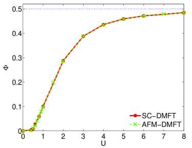
Figure 1: (Color online) Comparison of the anomalous expectation value $\Phi$ in the attractive model with the local magnetization $m_{A}$ in the AFM DMFT calculations for half filling.

We can see an excellent agreement of the corresponding expectation values from the two different calculations in all coupling regimes. In Fig. 2 we show the comparison for Green’s functions for $U=1,3,6$.

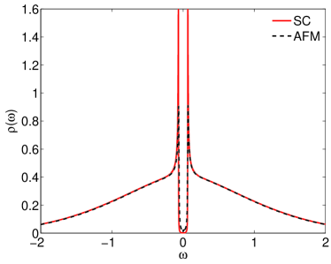
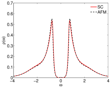
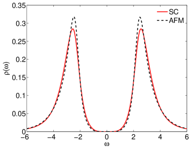
Figure 2: (Color online) Comparison of the spectral functions of SC-DMFT and AFM-DMFT calculations for $U=1,3,6$ (top, middle, bottom) for half filling.

We can see that for the whole frequency range the overall agreement of these spectral functions is good. In the weak coupling case, $U=1$, differences can be seen in the height of the quasiparticle peaks, which are sharper and higher in the calculation with superconducting order. In contrast, at strong coupling, $U=6$, the peaks are a bit broader and not as high as in the antiferromagnetic solution. It should be mentioned that for large $U$ DMFT-ED calculations in the AFM state have revealed spin polaron fine structure in the peaks Sangiovanni et al. (2006). These have so far escaped NRG calculations with less resolution at higher energy, but improved schemes might see this in the future. Generally, the results convey the picture of a good agreement for static and dynamic quantities for these two different DMFT-NRG calculations.

V Results for static and integrated quantities

Having tested the method at half filling we discuss results for different filling factors in this section. We present results for static and integrated quantities obtained with the extended DMFT-NRG method. They can be compared to the quantities obtained with DMFT calculations with other impurity solvers, like iterated perturbation theory (IPT)Garg et al. (2005) or EDToschi et al. (2005a). The semielliptic density of states with finite bandwidth $2D$ was used for all the following calculations,

$$\rho_{0}(\varepsilon)=\frac{2}{\pi D^{2}}\sqrt{D^{2}-\varepsilon^{2}},$$ (47)

with $D=2t$ for the Hubbard model. $t=1$ sets the energy scale in the following. All the results presented here are for $T=0$. For many of the calculations we take the model at quarter filling ($n=1/2$) as a generic case to analyze. For the NRG calculations we use $\Lambda=1.6$ and we keep 1000 states at each step. In the given units $U_{c}=2$ is the critical interaction for bound state formation in the two-body problem for the Bethe lattice Garg et al. (2005), and can be referred to as unitarity in analogy to the crossover terminology of the continuum system.

A starting point for an analysis of many quantities in the BCS-BEC crossover in the attractive Hubbard model can be mean field (MF) theory.Micnas et al. (1990) For a given $U$ and filling factor $n$ the chemical potential $\mu_{\rm MF}$ and the order parameter $\Delta_{\rm sc,MF}=U\Phi_{\rm MF}$ is determined by the mean field equations. The fermionic excitations are given by $E^{0}_{{\bm{k}}}=\sqrt{(\varepsilon_{{\bm{k}}}-\bar{\mu})^{2}+\Delta_{\rm sc,MF}{}^{2}}$ with $\bar{\mu}=\mu_{\rm MF}+Un/2$. At weak coupling the MF equations give the typical exponential behavior for $\Phi_{\rm MF}$, and for large $U$ one finds

$$\mu_{\rm MF}\simeq-\frac{1}{2}U,\qquad\Phi_{\rm MF}\simeq\frac{\sqrt{n(2-n)}}{2}.$$ (48)

If $\bar{\mu}$ is larger than the lower band energy (in our case $-D=-2$) then the minimal excitation energy is $\Delta_{\rm sc,MF}$ and occurs for $\varepsilon_{{\bm{k}}}=\bar{\mu}$, which usually applies for weak coupling. For strong coupling and $n\simeq 1$ the minimal excitation energy is also given by $\Delta_{\rm sc,MF}$, which is of order $U$. However, for low density, $n\to 0$, (48) yields $\bar{\mu}\to-U/2$, whereas $\Phi_{\rm MF}$ and thus $\Delta_{\rm sc,MF}$ are small. Once $\bar{\mu}$ has become smaller than the lower band energy, the minimal excitation energy is still of order $U$ as $E^{0}_{\min}=\sqrt{\bar{\mu}^{2}+\Delta_{\rm sc,MF}^{2}}=U$ independent of $n$. In the low-density strong-coupling limit the excitation gap is given by $\bar{\mu}$ which then corresponds to the energy of the two-fermion bound state.

The mean field spectral densities are given by

$$\rho^{\rm MF}_{{\bm{k}}}(\omega) = {u_{{\bm{k}}}^{2}}\delta(\omega-E^{0}_{{\bm{k}}})+{v_{{\bm{k}}}^{2}}\delta(\omega+E^{0}_{{\bm{k}}}),$$ (49)

$$\rho^{\rm MF,off}_{{\bm{k}}}(\omega) = {u_{{\bm{k}}}v_{{\bm{k}}}}[\delta(\omega-E^{0}_{{\bm{k}}})-\delta(\omega+E^{0}_{{\bm{k}}})],$$ (50)

where $u_{{\bm{k}}}^{2}=(1+(\varepsilon_{{\bm{k}}}-\bar{\mu})/{E^{0}_{{\bm{k}}}})/2$, $v_{{\bm{k}}}^{2}=1-u_{{\bm{k}}}^{2}$. There are two bands of quasiparticle excitations given by $\pm E_{{\bm{k}}}^{0}$, with weights $u_{{\bm{k}}}^{2}$ for particle-like and $v_{{\bm{k}}}^{2}$ for the hole-like excitations with infinite lifetime.

V.1 Behavior of the chemical potential

In Fig. 3 we plot our DMFT results for the chemical potential $\mu$ as a function of $U$ for different densities $n$.

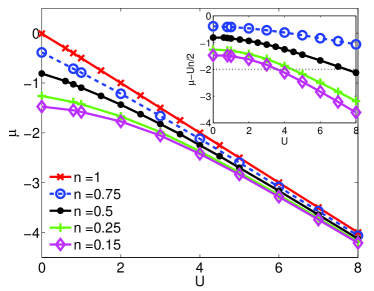
Figure 3: (Color online) The chemical potential $\mu$ as a function of $U$ for different filling factors $n$. The inset shows the quantity $\mu-Un/2$.

We can see that in all cases the values tend to the mean field value of $-U/2$ for large $U$. The results are in agreement with the ones reported by Garg et al.Garg et al. (2005), and as seen there also to the mean field values, which we did not include in the figure.

In the inset we show the quantity $\mu-Un/2$, which corresponds to $\bar{\mu}$ in the mean field theory. When the density is low, e.g. $n=0.15$, it is seen to intersect with the lower band edge $-2$ at intermediate interactions, $U\simeq 3.6$. Hence $\mu$ plays a role to determine the fermionic excitation spectrum as discussed before. If its value does not change much with temperature, and $\mu-Un/2$ remains smaller than $-D$, then no Fermi surface exists above $T_{c}$, and the system does not possess fermionic character anymore as fermions are bound to composite pairs also above $T_{c}$. For large $U$, $\mu\sim-U/2$ gives the binding energy.

V.2 Anomalous expectation value

One of the characteristic quantities of the superconducting state is the presence of a finite anomalous expectation value $\Phi$. The mean field equation gives an exponential increase for $\Phi$ at weak coupling, and a quantity which only depends on the density $n$ (48) in the strong coupling limit. In the attractive Hubbard model the $T_{c}$ increases exponentially with $U$ and then decreases at strong coupling with $t^{2}/U$ due to the kinetic term for hopping of fermionic pairs. This is captured in the DMFT calculation, which investigates the transition temperature as a pairing instability from the two particle response function.Keller et al. (2001) We expect the anomalous expectation value $\Phi$ in the strong coupling limit to be reduced from the mean field value due strong phase fluctuations. This is analogous to the reduction of the antiferromagnetic order parameter in the Heisenberg model by (transverse) spin waves. The latter are however not captured within our DMFT calculations in the state with broken symmetry, and $\Phi$ increases to a constant as in the mean field theory, as can be seen in Fig. 4 for quarter filling.

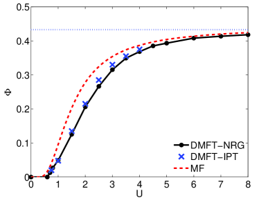
Figure 4: (Color online) The anomalous expectation value $\Phi$ as a function of $U$ for $n=0.5$. For comparison we have included the results from DMFT-IPT extracted from Ref. Garg et al., 2005 and the dashed line gives the result for $\Phi_{\rm MF}$.

The order parameter $\Delta_{\rm sc,DMFT}=U\Phi_{\rm DMFT}$ can, however, be interpreted as a high energy scale for pair formation then.Randeria (1995) The DMFT results for $\Phi_{\rm DMFT}$ are obtained by integration of the offdiagonal Green’s function as in equation (46) or the static expectation values calculated in the NRG procedure, the results of which are in very good agreement. MF and DMFT results show qualitatively a very similar overall behavior. There is a substantial reduction of the value through the quantum fluctuations included in the DMFT-NRG result, which appear most pronounced in the intermediate coupling regime, near unitarity $U_{c}=2$. However, also at weak coupling there is already a correction to the mean field results. For instance at $U=0.7$ we find $\Phi_{\rm MF}/\Phi_{\rm DMFT}\approx 2.58$. This is comparable to the reduction found in the analysis of Martín-Rodero and Flores Martin-Rodero and Flores (1992) with second order perturbation theory. Below $U=0.5$ the ordering scale is very small, and we do not find a well converged DMFT solution with symmetry breaking any more. In Fig. 4 we have also included the results obtained by DMFT-IPTGarg et al. (2005), which are slightly larger but otherwise in good agreement with our DMFT-NRG results.

V.3 Pair density

The ground state of the system is also characterized by the double occupancy $\langle n_{\uparrow}n_{\downarrow}\ \!\!\rangle$ or average pair density. The double occupancy multiplied by $U$ gives the expectation value of the potential energy. At weak coupling potential energy is gained in the symmetry broken state, whereas at strong coupling kinetic energy gain is usually responsible for Bose Einstein condensation. $\langle n_{\uparrow}n_{\downarrow}\ \!\!\rangle$ can be calculated directly from NRG expectation values. In Fig. 5 it is plotted for different filling factors for a range of interactions.

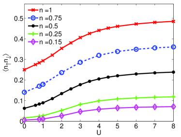
Figure 5: (Color online) Average pair density $\langle n_{\uparrow}n_{\downarrow}\ \!\!\rangle$ as a function of $U$ for a number of different filling factors.

In the non-interacting limit it is given by $(n/2)^{2}$, since the particles are uncorrelated and the probabilities $n/2$ to find a particle with spin $\sigma$ are just multiplied. In the strong coupling limit all particles are bound to pairs, and the pair density is given by half the filling factor, $\langle n_{\uparrow}n_{\downarrow}\ \!\!\rangle=n/2$. This continuous crossover from the non-interacting to the strong coupling values can be seen for all densities with the most visible change in the intermediate coupling regime occurring around $U_{c}=2$.

V.4 Momentum distribution

On the mean field level the weight of the quasiparticle peaks is given directly by the factors $u_{{\bm{k}}}^{2}$ and $v_{{\bm{k}}}^{2}$ as seen in equation (49). These factors also describe the momentum distribution $n^{\rm MF}_{{\bm{k}}}=v_{{\bm{k}}}^{2}$. The corresponding DMFT result for the momentum distribution is given by the integral over the diagonal Green’s function,

$$n_{{\bm{k}}}=\!\int\limits_{-\infty}^{0}\!\!{\rm d}\omega\;[-\mathrm{Im}G_{{\bm{k}}}(\omega)]/\pi.$$ (51)

In Fig. 6 we plot the momentum distribution $n_{{\bm{k}}}$ calculated from (51) in comparison with the mean field result for $n=0.5$.

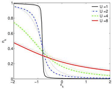
Figure 6: (Color online) The momentum distribution calculated from the ${\bm{k}}$-dependent Green’s function and compared with the MF result $n^{\rm MF}_{{\bm{k}}}=v_{{\bm{k}}}^{2}$ (dotted lines) for $n=0.5$.

For small attraction ($U=1$) we can see that $n_{{\bm{k}}}$ shows the typical form known from BCS theory dropping from one to zero in a small range around $\varepsilon_{{\bm{k}}}=\mu-Un/2$. Therefore, some momentum states above $\mu-Un/2$ are occupied, but only in a small region of the size of the order parameter. When $U$ is increased, the momentum distribution is spread over a larger range. In the BEC limit, where the fermions are tightly bound and therefore very localized in position space, we expect the momentum distribution to be spread due to the uncertainty principle. In all cases the sum rule $1/N\sum_{{\bm{k}}}n_{{\bm{k}}}=n/2$ is satisfied numerically within an accuracy of about 1%. There are visible quantitative deviation between MF and DMFT results, but they are fairly small. Our results comparable well to the ones presented by Garg et al. Garg et al. (2005).

In the experiments in ultracold gases where the BCS-BEC crossover is investigated the momentum distribution can be measured quite accurately. This has been studied also in comparison with mean field results by Regal et al.Regal et al. (2005). Considering low densities for the lattice system, and taking into that an additional broadening would occur at finite temperature, a qualitative agreement of our results with the experiment can be found.

V.5 Superfluid stiffness

For a system in a coherent superfluid state another characteristic quantity is the superfluid stiffness $D_{s}$. It is a measure of the energy required to twist the phase of the condensate, and therefore related to the degree of phase coherence of the superconducting state. Usually, it is proportional to the superfluid density $n_{s}$, which is experimentally accessible via the penetration length. Toschi et al.Toschi et al. (2005a) have investigated the relation between $T_{c}$ and $D_{s}$ in the attractive Hubbard model and found that a linear scaling relation, as in the Uemura plot, holds at intermediate and strong coupling.

$D_{s}$ can be calculated either from the weight of the delta-function in the optical conductivity or from the transverse part of the current-current correlation functionToschi et al. (2005a) $\chi_{j_{\perp};j_{\perp}}(\bm{q},\omega)$,

$$D_{s}=D_{\rm dia}-\chi_{j_{\perp};j_{\perp}}(\bm{q}\to 0,\omega=0)$$ (52)

The diamagnetic term $D_{\rm dia}$ is essentially given by the kinetic energy,

$$D_{\rm dia}=-\frac{2}{\beta}\sum_{n}\!\int\limits\!\!{\rm d}\varepsilon_{{\bm{k}}}\;\rho_{0}(\varepsilon_{{\bm{k}}})\varepsilon_{{\bm{k}}}G_{{\bm{k}}}(i\omega_{n}),$$ (53)

where $G_{{\bm{k}}}(i\omega_{n})$ is the Matsubara Green’s function. In the infinite dimensional limit $\chi_{j_{\perp};j_{\perp}}$ reduces to the bubble of normal and anomalous propagators Toschi et al. (2005a); Pruschke et al. (1993). From this and the relation $-\partial/\partial\varepsilon_{{\bm{k}}}[\rho_{0}(\varepsilon_{{\bm{k}}})V(\varepsilon_{{\bm{k}}})]=\rho_{0}(\varepsilon_{{\bm{k}}})\varepsilon_{{\bm{k}}}$ and integration by parts one finds that the diamagnetic term cancels, which yieldsToschi et al. (2005a)

$$D_{s}=\frac{4}{\beta}\sum_{n}\!\int\limits\!\!{\rm d}\varepsilon_{{\bm{k}}}\;\rho_{0}(\varepsilon_{{\bm{k}}})V(\varepsilon_{{\bm{k}}})G_{{\bm{k}}}^{\rm off}(i\omega_{n})G_{{\bm{k}}}^{\rm off}(i\omega_{n}),$$ (54)

where $V(\varepsilon_{{\bm{k}}})=(4t^{2}-\varepsilon_{{\bm{k}}}^{2})/3$ for the Bethe lattice. We can use the spectral representation,

$$G_{{\bm{k}}}^{\rm off}(i\omega_{n})=\!\int\limits\!\!{\rm d}\omega^{\prime}\;\frac{\rho_{{\bm{k}}}^{\rm off}(\omega^{\prime})}{i\omega_{n}-\omega^{\prime}}$$ (55)

and the Kramers-Kronig relations for the real and imaginary parts of the Green’s function such that at zero temperature $D_{s}$ takes the form,

$$D_{s}=-\frac{8}{\pi}\!\int\limits\!\!{\rm d}\varepsilon_{{\bm{k}}}\;\rho_{0}(\varepsilon_{{\bm{k}}})V(\varepsilon_{{\bm{k}}})\!\int\limits_{-\infty}^{0}\!\!{\rm d}\omega\;\mathrm{Im}G_{{\bm{k}}}^{r,\rm off}(\omega)\mathrm{Re}G_{{\bm{k}}}^{r,\rm off}(\omega),$$ (56)

where $G_{{\bm{k}}}^{r,\rm off}(\omega)$ is the retarded offdiagonal Green’s function (5). We can evaluate the expression (56) using the mean field Green’s function in the form (50), which yields the somewhat simpler expression

$$D^{\rm MF}_{s}=4\!\int\limits_{-D}^{D}\!\!{\rm d}\varepsilon_{{\bm{k}}}\;\rho_{0}(\varepsilon_{{\bm{k}}})V(\varepsilon_{{\bm{k}}})\frac{u_{{\bm{k}}}^{2}v_{{\bm{k}}}^{2}}{E_{{\bm{k}}}^{0}}.$$ (57)

This expression can be evaluated in the limit $U\to 0$, $\Delta_{\rm sc}\to 0$ as ${u_{{\bm{k}}}^{2}v_{{\bm{k}}}^{2}}/{E_{{\bm{k}}}^{0}}$ goes to a delta function then, and hence $D_{s}\to 2\rho_{0}(\bar{\mu})V(\bar{\mu})$.

In Fig. 7 the superfluid stiffness $D_{s}$ calculated from equation (56) is displayed as a function of $U$ for quarter filling. The dashed line shows the result as obtained from equation (57), where the mean field Green’s functions are used to evaluate the integrals.

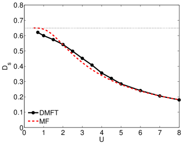
Figure 7: (Color online) The superfluid stiffness $D_{s}$ as calculated from the offdiagonal Green’s function in equation (56) for $n=0.5$. The dashed line gives the result for $D_{s}$, when evaluated as in (57).

We can see that the results for $D_{s}$ of DMFT and MF calculation do not deviate very much. The superfluid stiffness is maximal in the BCS limit and decreases to smaller values in the BEC limit. $D_{s}$ is proportional to the inverse of the effective mass of the pairs $m_{B}\sim U/t^{2}$, and therefore expected to decrease like $1/U$. The system in this limit consists of heavy, weakly interacting bosons, with less phase coherence. The results shown are in agreement with the ones reported by Toschi et al.Toschi et al. (2005a).

Summarizing this section, we see that our DMFT-NRG results for chemical potential, static and integrated properties at zero temperature are in good agreement with earlier calculations based on different impurity solvers. In fact most of the results are in good agreement with mean field theory and quantitative deviations due to the fluctuations included in DMFT are not very large. One could therefore argue that the main features are already fairly well described by the simpler static mean field treatment. In the next section we will turn to spectral quantities. In contrast there certain features like the distinction of coherent and incoherent excitations can only be described when we go beyond the mean field theory. Some of these extra features found in the spectral resolution are lost again when considering integrated quantities.

VI Spectral functions

In this section we present our DMFT-NRG results for the local spectral density $\rho(\omega)$ and the ${\bm{k}}$-resolved spectra, $\rho_{{\bm{k}}}(\omega)=-\mathrm{Im}G_{{\bm{k}}}(\omega)/\pi$, in the different parameter regimes. Before discussing these results in detail, and comparing them with those of Garg et al.Garg et al. (2005), we consider the different types of approximations used in the IPT and NRG calculations. These are relevant in assessing the two sets of results to arrive at a clearer physical interpretation.

The approximation used in the IPT is in restricting the calculation to the second order diagram for the self-energy. This is evaluated using the Hartree-Bogoliubov corrected propagator for the effective impurity. If this propagator has a spectral density with a gap $E_{g}$, then imaginary part of the self-energy from this second order scattering term can only develop in the regime $|\omega|>3E_{g}$. This threshold energy of $3E_{g}$ corresponds to the minimum energy for a fermion above the gap $E_{g}$ to emit a quasiparticle-quasihole pair excitation. Therefore, in the IPT the single-particle spectral functions $\rho_{{\bm{k}}}(\omega)$ have isolated delta-function peaks corresponding to the Bogoliubov quasiparticle excitations with minimal energy $E_{g}$, together with incoherent continuous spectrum for $|\omega|>3E_{g}$.

In applying the NRG approach to the effective impurity problem, approximations arise in using a discrete spectrum for the conduction electron bath. The spectral functions are calculated as Lehmann sums over delta-function peaks, the positions of the peaks being deduced from the discrete many-body energy levels and their weighting from the corresponding matrix elements. This is also the case for other methods using numerical diagonalization such as the ED (exact diagonalization) method. To obtain a continuous spectral function these delta-function peaks have to be broadened appropriately, usually with a lognormal function with parameter $b$ Bulla et al. (2008). If the broadening is too large certain features blur, if it is too small the spectral functions has many spikes and is difficult to interpret. With such a broadening procedure it is difficult to resolve sharp features such as a gap in the spectrum and hence an energy $E_{g}$. However, usually an estimate of the gap can be made when the broadening is taken into account. For all the previous results on static and integrated quantities we have used a conventional broadening parameter $b=0.5$, and the results for these quantities depend very little on the broadening. In this section we use smaller values in order to avoid missing features which can be lost with the larger broadening parameter.

Another aspect of the NRG calculations that can lead to some numerical uncertainty is in the way the self-energy is calculated. In equation (73) it is shown how the self-energy can be calculated from the matrices of the Green’s function $\underline{G}$ and the higher Green’s function $\underline{F}$. If one is interested in the values of $\omega$ for which the imaginary part of the self-energy vanishes then the whole expression in equation (73) has to be considered. As is well known for NRG calculations for the Anderson impurity model Bulla et al. (2008) the condition $\mathrm{Im}\Sigma(0)=0$ for the Friedel sum rule can be reasonably well satisfied. However, $\mathrm{Im}\Sigma$ is never exactly zero and numerical errors can often be seen in small imaginary parts of the self-energy from this procedure.

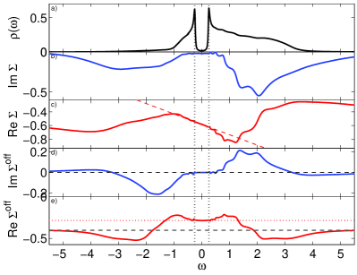
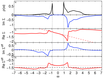
Figure 8: (Color online) The spectral functions, imaginary and real parts of the diagonal and offdiagonal self-energies plotted for $U=2$ (top) and $U=4$ (bottom) with $b=0.2$, $n=0.5$. The dotted vertical line gives the peak position of the spectral function, which can be roughly identified with $E_{g}$.

In Fig. 8 we present the NRG results for the local spectral density $\rho(\omega)$ and the real and imaginary parts for the diagonal and offdiagonal self-energies for $U=2$ and $U=4$. We see that $\mathrm{Im}\Sigma$ and $\mathrm{Im}\Sigma^{\rm off}$ are approximately zero for a certain range of $\omega$ for both for $U=2$ and $U=4$. $\mathrm{Im}\Sigma^{\rm off}$ is an antisymmetric function, which has peaks at similar position as $\mathrm{Im}\Sigma$. $\mathrm{Re}\Sigma^{\rm off}$ is a symmetric function which for large $\omega$ tends to the value $\Delta_{\rm sc}=U\Phi$ of the interacting system (46) and for small $\omega$ can be interpreted as a renormalized gap.

In the weaker coupling case $U=2$ we find a trend similar to the IPT in that $\mathrm{Im}\Sigma$ deviates appreciably from zero only when $|\omega|>3E_{g}$. This can be seen on closer inspection of the top part of Fig. 8, where we estimate $E_{g}\approx 0.25$, and $\mathrm{Im}\Sigma>0$ for roughly $\omega>0.75$ (the wiggles for smaller $\omega$ are interpreted as inaccuracies). This means that in the corresponding spectrum for $\rho_{{\bm{k}}}(\omega)$ there are isolated quasiparticle peaks and a continuous incoherent part in the spectrum for $|\omega|>3E_{g}$. The widths of the quasiparticles peaks, however, will not be precisely zero as in the IPT due to the very small imaginary parts. In the spectrum for $\rho(\omega)$ and $U=2$ shown in Fig. 8 there is a sharp peak due to the quasiparticle excitations in $\rho(\omega)$ just above the gap (see also Fig. 1 in Ref. Bauer and Hewson, 2009). This quasiparticle band is very similar to the one based on IPT presented in Fig. 3 in Ref. Garg et al., 2005. In the IPT case there is a square root singularity at the gap edge which does not appear in the NRG results due to the small imaginary part in the self-energies.

This picture changes in the stronger coupling case $U=4$. Here it can be seen the imaginary parts of both the diagonal and off-diagonal self-energies develop a pronounced peak which falls within the region, $E_{g}<|\omega|<3E_{g}$. This leads to incoherent spectral weight in $\rho_{{\bm{k}}}(\omega)$ for $|\omega|<3E_{g}$. This is a difference with the IPT results where the imaginary parts of the self-energy are always zero for $E_{g}<|\omega|<3E_{g}$ and consequently there is no incoherent part of the spectrum for $\rho_{{\bm{k}}}(\omega)$ in the range $|\omega|<3E_{g}$. An explanation for this difference can be seen by examining what happens to the local dynamical charge susceptibility $\chi_{c}(\omega)$ as $U$ increases. Results for $\chi_{c}(\omega)$ for $U=3,4,6$ are shown Fig. 9. The excitation gap $\Delta_{c}$ in this spectrum can be seen to decrease significantly as $U$ increases. In Ref. Bauer and Hewson, 2009 it was found that at strong coupling $\Delta_{c}$ decreases like $\sim t^{2}/U$. In the weak coupling case $\Delta_{c}\sim 2E_{g}$, but for strong coupling $E_{g}$ increases with $U$, while $\Delta_{c}$ decreases. Therefore, the contribution to the self-energy arising from the scattering with charge fluctuations can, for larger $U$, generate a finite imaginary part of the self-energy for $E_{g}<|\omega|<3E_{g}$. The location of the peak in $\mathrm{Im}\Sigma$ appears consistent with such an interpretation. The same effect cannot arise from scattering with the spin fluctuations, as these have a larger characteristic energy scale (of the order of $U$). For a further discussion of the behavior of the charge and spin gap we refer to Ref. Bauer and Hewson, 2009.

The development of the peak in the imaginary part of the self-energy in the range $|\omega|<3E_{g}$ leads to a dip in the local spectral function $\rho(\omega)$ for $U=4$ as can be seen in Fig. 8. There is then a peak-dip-hump structure in $\rho(\omega)$ for $U=4$ (see also Fig. 11). This feature has also been found in calculations for the attractive continuum model Pieri et al. (2004). This behavior is not visible in the IPT calculations (cf. Fig. 3 in Ref. Garg et al., 2005). The most likely explanation is the restriction in the IPT to the second order diagram, which does not allow for any renormalization of the charge fluctuations.

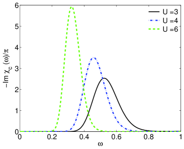
Figure 9: (Color online) The imaginary part of the local charge susceptibility for $U=3,4,6$ ($b=0.2$). We find strong excitations corresponding to charge fluctuations there below the respective estimates of $E_{g}\simeq 0.5,0.9,1.7$.

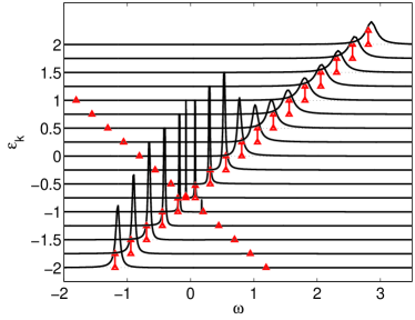
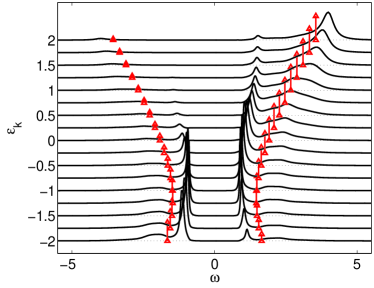
Figure 10: (Color online) The $\varepsilon_{{\bm{k}}}$-resolved spectral functions $\rho_{{\bm{k}}}(\omega)$ for quarter filling in the BCS-limit, $U=1$ (top), and towards the BEC limit, $U=4$ ($b=0.2$) (bottom). The arrows show the delta-function peaks of the mean field solution $\rho^{0}_{{\bm{k}}}(\omega)$, where the height of the arrow indicates the weight of the peak.

We now consider the effect of increasing $U$ on the quasiparticle excitations which can be seen in the results for the spectral function $\rho_{{\bm{k}}}(\omega$) for $U=1$ and $U=4$ for quarter filling shown in Fig. 10. For both cases, $U=1$ and $U=4$, we can see a series of sharp quasiparticle peaks which are most narrow in the region $\varepsilon_{{\bm{k}}}\approx\bar{\mu}$, which is also the point where the spectral gap is minimal. In the latter case $U=4$ in addition we find the hump with incoherent spectral weight as discussed earlier for $\rho(\omega)$. We have also added arrows which indicate the position of the quasiparticle peaks $\pm E_{{\bm{k}}}^{0}$ in mean field theory (49), and the height gives the spectral weight. We can see that they describe the position of the quasiparticle excitation well for $U=1$. For the larger $U$ case the structure in the spectral function is not so well captured by the single quasiparticle peaks of the mean field theory. The energy of the quasiparticle excitations differ markedly from the mean field prediction and there is a significant transfer of spectral weight to the incoherent hump, in particular at high energy. The quasiparticle band (weight and band width) at low energy is, however, captured on a qualitative level by mean field theory. The quasiparticle peaks for $\rho_{{\bm{k}}}(\omega)$ always have a finite width since our self-energy is never strictly zero. One can infer the bands from the poles of the Green’s function $E_{{\bm{k}}}$ and compare them with the mean field bands $\pm E_{{\bm{k}}}^{0}$. For the weak coupling they are in good agreement. Towards the BEC limit the effective mass $m_{B}$ of a boson pair is of order $U$. This is reflected in the smaller effective band width for the case $U=4$ (Fig. 10). The weight of the peaks in the full spectrum $\rho_{{\bm{k}}}(\omega)$ is in accordance with the height of the arrows for $\rho^{0}_{{\bm{k}}}(\omega)$. We can see that in the BCS limit (top) the weight in the lower band decreases rapidly to zero near $\varepsilon_{{\bm{k}}}=\bar{\mu}$, whereas towards the BEC limit (bottom) it spreads over a much larger region which corresponds to what has been observed for momentum distributions in Fig. 6.

In earlier work Bauer and Hewson (2009) the quasiparticle properties were analyzed in an expansion around the solutions $E_{{\bm{k}}}$ of the equation $\mathrm{Re}G_{{\bm{k}}}(\omega=E_{{\bm{k}}})^{-1}=0$. This led to the Lorentz-like quasiparticle peak of the form

$$\rho_{{\bm{k}}}(\omega)=w_{+}(E_{{\bm{k}}})\frac{W(E_{{\bm{k}}})/\pi}{(\omega-E_{{\bm{k}}})^{2}+W(E_{{\bm{k}}})^{2}},$$ (58)

with width $W(E_{{\bm{k}}})$ and weight $w_{+}(E_{{\bm{k}}})$. When a standard broadening of $b=0.5$ is used one finds a finite width of the peaks which increases in the crossover regime leading to a strongly reduced life time of the quasiparticles. In the more careful analysis here with smaller broadening and taking into account possible errors in determining the self-energy we come to the conclusion that this is not generally correct. We should not expect a finite imaginary part of the self-energy to appear for $\omega\simeq E_{g}$ in a DMFT calculation which does not include collective modes.

Being aware of limitations in our numerical calculations we investigate in more detail how the one-particle spectra near the minimal spectral gap modify from weak to intermediate coupling. Here we use a general scheme in which we analyze the peaks in the spectral function directly numerically and estimate the transfer of weight from the quasiparticle peaks to the incoherent part of the spectrum. We take the peak position in $\rho_{{\bm{k}}}(\omega)$ for a given $\varepsilon_{{\bm{k}}}$ as the excitation energy $E^{\rm ex}_{{\bm{k}}}$, the full width $F_{\rm peak}$ at half maximum as the width and the weight is determined by the integration over a region around $E^{\rm ex}_{{\bm{k}}}$ of $2F_{\rm peak}$. Such an analysis also applies to antisymmetric peak forms, and is equivalent to the other one for sharp Lorentz-like peaks. Note that a normalized Lorentz peak with width $\Delta$ (half width at half maximum) integrated from $-2\Delta$ to $2\Delta$ yields the spectral weight $w_{2\Delta}=2\arctan(2)/\pi\approx 0.705$.

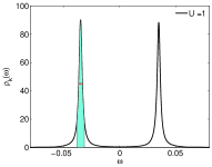
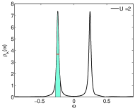
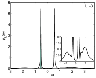
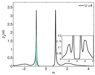
Figure 11: (Color online) The spectral functions $\rho_{{\bm{k}}}(\omega)$ for an $\varepsilon_{{\bm{k}}}$ where the gap is minimal for quarter filling and $U=1-4$ ($b=0.2$). The integration area, which gives the weight of the peaks is shown.

We have done such an analysis for the $\varepsilon_{{\bm{k}}}$-resolved spectral functions, where we consider an $\varepsilon_{{\bm{k}}}$ such that the excitation gap is minimal. The corresponding spectral functions for $U=1-4$ are displayed in Fig. 11. We have included a line at half maximum for the width as well as marked the integration area in the low energy peak. We can see now very clearly how the spectrum changes from one coherent quasiparticle peak at weak coupling to the peak-dip-hump structure at intermediate coupling. This is similar to what was found in the calculation for an attractive continuum model Pieri et al. (2004), where a sharp quasiparticle peak with little weight is still present at strong coupling. In our calculation the strong coupling limit is not easy to analyze as we always have some finite imaginary part of the self-energy leading to a finite width of the quasiparticle peak, which is partly spurious and tends to be larger at large coupling. At strong coupling the excitations occur at higher energy and we have to reduce the broadening further, which leads to a more spiky spectrum. It should be mentioned that if the broadening is chosen larger (e.g. $b=0.5$) then there is only one broad peak in the spectral function.

The estimate of the weight of the quasiparticle peak $w_{\rm peak}$ extracted by integration is plotted in Fig. 12 as a function of $U$. For weak coupling, $U\simeq 1$, we would expect the mean field result $v^{2}_{{\bm{k}}}(\varepsilon_{{\bm{k}}}=\bar{\mu})=0.5$. Due to the reduced integration range we find $w_{\rm peak}\approx 0.34$, but division by $w_{2\Delta}$ gives a value close to $0.5$ .

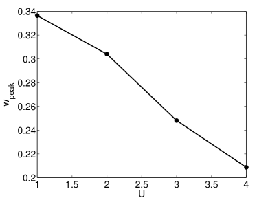
Figure 12: The weight of the peak for spectral excitation as a function of $U$ for quarter filling.

Coming from weak coupling we find a decrease as spectral weight is transferred to incoherent parts as seen before in Fig. 11. This resembles the results of Ref. Pieri et al., 2004.

As discussed before due to the uncertainty about the imaginary part of the self-energy at low frequency the behavior of the width $F_{\rm peak}$ can not be reliably estimated. At weak coupling we expect the prediction of a real delta-function with $F_{\rm peak}\to 0$ to hold. Whether at strong coupling low enough excitations can be generated to change this remains to be answered. We stress here again that the conclusions about the behavior of $W(\min E_{{\bm{k}}})$ as given in (58), which was reported in Fig. 3 of Ref. Bauer and Hewson, 2009, are found to be incorrect as judged by the present more careful interpretation of our DMFT-NRG calculations.

VII Conclusions

In this paper we have presented an analysis of the ground state properties of the attractive Hubbard model in the symmetry broken phase in the BCS-BEC crossover. The emphasis has been on the evolution of spectral functions in the crossover regime. Our analysis is based on an extension of the DMFT-NRG method to the case with superconducting symmetry breaking. We have given many details of this extension in section III and the appendix. At half filling we have related our approach both for the effective impurity model and for the lattice quantities to earlier DMFT-NRG calculations with antiferromagnetic symmetry breaking. A good agreement has been found there, which validates the applicability of our approach. As emphasized in Ref. Bauer and Hewson, 2009, apart from the attractive Hubbard model the extended method can be useful to study superconductivity in other models, such as the Hubbard-Holstein type, and also questions related to the microscopic description of magnetic impurities in superconductors, which require self-consistent treatments.

We have discussed our DMFT-NRG results for static and integrated quantities, like the anomalous expectation value, the double occupancy or superfluid stiffness. The results for these are in good agreement with earlier calculations based on different impurity solvers, and it has been found that most of the results are already obtained qualitatively well on the mean field level.

The main interest of this paper has been to study the fermionic spectrum throughout the crossover regime. The local dynamics are very well described in our DMFT-NRG approach. We discussed how the behavior of the dynamic self-energies changes when the interaction becomes larger. At weak coupling the spectrum is dominated by sharp symmetric Bogoliubov quasiparticle peaks as known from mean field theory. Contributions from particle-particle and particle-hole fluctuations incorporated in the dynamic self-energies appear at higher energy and are small, similar to those seen in the IPT approach. However, when the local interaction is in the unitary regime and larger, the imaginary part of the dynamic self-energy shows a characteristic feature which generates a peak-dip-hump structure in the spectral function. We argued that this features is likely to be generated by charge fluctuations as seen in the local dynamic charge susceptibility. One finds that spectral weight is transferred into the incoherent parts (hump) of the spectrum on increasing the coupling.

To answer the question whether at strong coupling the fermionic quasiparticles acquire a finite width one needs clarify over which region the imaginary parts of the self-energies vanish. Unfortunately, our method, in which spectral functions are obtained after broadening delta-peaks, is not accurate enough at present to allow for definite statements. It is possible that the peaks always remain sharp in the limit of infinite dimensions. Our DMFT approach does not capture spatial fluctuations and the gapless Goldstone mode. It would also be of great interest to study how such effects give a modification of the discussed fermionic spectrumBorejsza and Dupuis (2003, 2004) and possibly a suppression of the quasiparticle peaks.

Acknowledgment

We wish to thank W. Metzner, A. Oguri, P. Strack and A. Toschi for helpful discussions, W. Koller and D. Meyer for their earlier contributions to the development of the NRG programs, and R. Zeyher for critically reading the manuscript.

Appendix A NRG formalism with superconducting symmetry breaking

A.1 Mapping to the linear chain

The second important step (ii) in the self-consistent NRG procedure is to map the discretized model (13) to the so-called linear chain model of the general form (28),

$$H_{\mathrm{And}} = \sum_{\sigma,n=0}^{N}\varepsilon_{n}f^{\dagger}_{n,\sigma}f_{n,\sigma}+\sum_{{\sigma},n=-1}^{N}\beta_{n}(f^{\dagger}_{n,\sigma}f_{n+1,\sigma}$$ (59)

$$+\mathrm{h.c.})-\sum_{n=0}^{N}\Delta_{n}(f^{\dagger}_{n,\uparrow}f^{\dagger}_{n,\downarrow}+f_{n,\downarrow}f_{n,\uparrow}).$$

The orthogonal transformation has been chosen in the form (cf. equation (31)),

$$f_{n,\uparrow} = \sum_{\alpha,m}u_{\alpha,nm}a_{\alpha,m,\uparrow}-v_{\alpha,nm}a_{\alpha,m,\downarrow}^{\dagger},$$ (60)

$$a_{\alpha,m,\uparrow} = \sum_{n}u_{\alpha,nm}f_{n,\uparrow}+v_{\alpha,nm}f_{n,\downarrow}^{\dagger},$$ (61)

$$f_{n,\downarrow}^{\dagger} = \sum_{\alpha,m}v_{\alpha,nm}a_{\alpha,m,\uparrow}+u_{\alpha,nm}a_{\alpha,m,\downarrow}^{\dagger},$$ (62)

$$a_{\alpha,m,\downarrow}^{\dagger} = \sum_{n}-v_{\alpha,nm}f_{n,\uparrow}+u_{\alpha,nm}f_{n,\downarrow}^{\dagger}.$$ (63)

The matrix elements of the transformation obey the relations

$$\sum_{n}u_{\alpha,nm}u_{\alpha^{\prime},nm^{\prime}}+v_{\alpha,nm}v_{\alpha^{\prime},nm^{\prime}} = \delta_{m,m^{\prime}}\delta_{\alpha,\alpha^{\prime}},$$

$$\sum_{m,\alpha}u_{\alpha,nm}u_{\alpha,n^{\prime}m}+v_{\alpha,nm}v_{\alpha,n^{\prime}m} = \delta_{n,n^{\prime}},$$

and

$$\sum_{m,\alpha}u_{\alpha,nm}v_{\alpha,n^{\prime}m}-v_{\alpha,nm}u_{\alpha,n^{\prime}m} = 0,$$

$$\sum_{n}u_{\alpha,nm}v_{\alpha^{\prime},nm^{\prime}}-v_{\alpha,nm}u_{\alpha^{\prime},nm^{\prime}} = 0,$$

which ensure that both operator sets satisfy canonical anticommutation relations. We can now derive the recursion relations for the matrix elements and the parameters. This is done in analogy to earlier work by Bulla et al. Bulla et al. (1997). We equate the representations for the media of (13) and (59) and substitute the operator transformation (60)-(63). One can then read off the coefficients of the $f_{n,\uparrow}$-operators ($n>0$) on both sides of the equation, which yields

$$\sum_{n^{\prime},\alpha}\xi^{\alpha}_{n^{\prime}}\Big{(}u_{\alpha,nn^{\prime}}a_{\alpha,n^{\prime},\uparrow}^{\dagger}+v_{\alpha,nn^{\prime}}a_{\alpha,n^{\prime},\downarrow}\Big{)}$$

$$+\sum_{n^{\prime},\alpha}\delta_{n^{\prime}}^{\alpha}\Big{(}v_{\alpha,nn^{\prime}}a_{\alpha,n^{\prime},\uparrow}^{\dagger}-u_{\alpha,nn^{\prime}}a_{\alpha,n^{\prime},\downarrow}\Big{)}=$$

$$=\varepsilon_{n}f_{n,\uparrow}^{\dagger}+\beta_{n-1}f_{n-1,\uparrow}^{\dagger}+\beta_{n}f_{n+1,\uparrow}^{\dagger}-\Delta_{n}f_{n,\downarrow}.$$

From this we find the expression (33) for $\varepsilon_{n}$ by taking the anticommutator with $f_{n,\uparrow}$. The anticommutator with $f^{\dagger}_{n,\downarrow}$ gives expression (34) for $\Delta_{n}$. With the representations (60)-(63) we can modify the equation (A.1) to obtain

$$\beta_{n}f_{n+1,\uparrow}^{\dagger} = \sum_{n^{\prime},\alpha}\Big{[}(\xi^{\alpha}_{n^{\prime}}-\varepsilon_{n})u_{\alpha,nn^{\prime}}+(\delta_{n^{\prime}}^{\alpha}+\Delta_{n})v_{\alpha,nn^{\prime}}$$

$$-\beta_{n-1}u_{\alpha,n-1n^{\prime}}\Big{]}a_{\alpha,n^{\prime},\uparrow}^{\dagger}$$

$$+ \sum_{n^{\prime},\alpha}\Big{[}(\Delta_{n}-\delta_{n^{\prime}}^{\alpha})u_{\alpha,nn^{\prime}}+(\xi^{\alpha}_{n^{\prime}}+\varepsilon_{n})v_{\alpha,nn^{\prime}}+$$

$$\beta_{n-1}v_{\alpha,n-1n^{\prime}}\Big{]}a_{\alpha,n^{\prime},\downarrow}.$$

By comparison with (31) we can read off a recursion relation for $u_{\alpha,n+1n^{\prime}}$ in equation (36) and for $v_{\alpha,n+1n^{\prime}}$ as in equation (37). The recursion relation for $\beta_{n}$ is obtained from the anticommutator of with $f_{n+1,\uparrow}$ which yields

$$\beta_{n}^{2}=\sum_{n^{\prime},\alpha}(u_{\alpha,n+1n^{\prime}}^{2}+v_{\alpha,n+1n^{\prime}}^{2}).$$

With the orthonormality relations and the definitions $\varepsilon_{n}$ and $\Delta_{n}$ we can find the expression in equation (35).

A.2 Relevant Green’s functions

In this section we briefly outline some details for the calculations of the relevant Green’s functions and the self-energy for completeness.Bauer et al. (2007) For the Green’s functions it is convenient to work in Nambu space, $\bm{C}^{\dagger}_{d}=(d^{\dagger}_{\uparrow},d_{\downarrow})$, with $2\times 2$ matrices. The relevant retarded Green’s functions are then

$$\underline{G}_{d}(\omega)=\langle\!\langle\bm{C}_{d};\bm{C}^{\dagger}_{d}\rangle\!\rangle_{\omega}=\left(\begin{array}[]{c c}\langle\!\langle d_{\uparrow};d^{\dagger}_{\uparrow}\rangle\!\rangle_{\omega}&\langle\!\langle d_{\uparrow};d_{\downarrow}\rangle\!\rangle_{\omega}\\ \langle\!\langle d^{\dagger}_{\downarrow};d^{\dagger}_{\uparrow}\rangle\!\rangle_{\omega}&\langle\!\langle d^{\dagger}_{\downarrow};d_{\downarrow}\rangle\!\rangle_{\omega}\end{array}\right).$$ (64)

In the NRG approach we calculate $G_{11}$ and $G_{21}$ directly and infer $G_{22}(\omega)=-G_{11}(-\omega)^{*}$, which follows from $G_{A,B}^{\rm ret}(\omega)=-G_{B,A}^{\rm adv}(-\omega)$ and $G_{A,B}^{\rm ret/adv}(\omega)=-G_{A^{\dagger},B^{\dagger}}^{\rm ret/adv}(-\omega)^{*}$ for fermionic operators $A$, $B$. Similarly, we can find $G_{12}(\omega)=G_{21}(-\omega)^{*}$. In the derivation one has to be careful and include a sign change for up down spin interchange in the corresponding operator combination.

In the non-interacting case we can deduce the $d$-site Green’s function matrix of the model Hamiltonian (6) exactly. To do so we rewrite the superconducting term of the medium $H_{\rm sc}$ by introducing the vector of operators and the symmetric matrix

$$\bm{C}_{{\bm{k}}}:=\left(\begin{array}[]{c}\!c_{{\bm{k}},\uparrow}\\ \!c^{\dagger}_{-{\bm{k}},\downarrow}\end{array}\right),\qquad A_{{\bm{k}}}:=\left(\begin{array}[]{cc}\!\varepsilon_{{\bm{k}}}&\!-\Delta_{{\bm{k}}}\\ \!-\Delta_{{\bm{k}}}&\!-\varepsilon_{{\bm{k}}}\end{array}\right).$$ (65)

Then $H_{\rm sc}$ can be written as

$$H_{\rm sc}=\sum_{{\bm{k}}}\bm{C}_{{\bm{k}}}^{\dagger}A_{{\bm{k}}}\bm{C}_{{\bm{k}}}.$$ (66)

The matrix Green’s function in the superconducting bath is then given by $\underline{g}_{{\bm{k}}}(i\omega_{n})=(i\omega_{n}\mathbbm{1}_{2}-A_{{\bm{k}}})^{-1}$,

$$\underline{g}_{{\bm{k}}}(i\omega_{n})^{-1}=i\omega_{n}\mathbbm{1}_{2}-\varepsilon_{{\bm{k}}}\tau_{3}+\Delta_{{\bm{k}}}\tau_{1},$$ (67)

where $\tau_{i}$ are Pauli matrices. It follows that

$$\underline{g}_{{\bm{k}}}(i\omega_{n})=\frac{i\omega_{n}\mathbbm{1}_{2}+\varepsilon_{{\bm{k}}}\tau_{3}-\Delta_{\rm sc}\tau_{1}}{(i\omega_{n})^{2}-(\varepsilon_{{\bm{k}}}^{2}+\Delta_{{\bm{k}}}^{2})}.$$ (68)

In the non-interacting case for $T=0$, we have therefore

$$\underline{G}^{0}_{d}(\omega)^{-1}=\omega\mathbbm{1}_{2}-\varepsilon_{d}\tau_{3}-\sum_{{\bm{k}}}V_{{\bm{k}}}^{2}\tau_{3}\underline{g}_{{\bm{k}}}(i\omega_{n})\tau_{3}.$$ (69)

The local full Green’s function matrix $\underline{G}_{d}(\omega)^{-1}$ for the effective impurity model is given by the Dyson matrix equation

$$\underline{G}_{d}(\omega)^{-1}=\underline{G}_{0}^{-1}(\omega)-\underline{\Sigma}(\omega),$$ (70)

where $\underline{\Sigma}(\omega)$ is the self-energy matrix.

A.3 Self-energy using the higher $F$-Green’s function

As described by Bulla et al. Bulla et al. (1998) there is a method to calculate the self-energy employing a higher $F$-Green’s function, and it can also be used for the case with superconducting bath. The calculation taking into account all offdiagonal terms yields the following matrix equation

$$\underline{G}^{0}_{d}(\omega)^{-1}\underline{G}_{d}(\omega)-U\underline{F}(\omega)=\mathbbm{1}_{2},$$ (71)

with the matrix of higher Green’s functions $\underline{F}(\omega)$,

$$\underline{F}(\omega)=\left(\begin{array}[]{c c}F_{11}(\omega)&F_{12}(\omega)\\ F_{21}(\omega)&F_{22}(\omega)\end{array}\right).$$ (72)

We have introduced the matrix elements $F_{11}(\omega)=\langle\!\langle d_{\uparrow}n_{\downarrow};d^{\dagger}_{\uparrow}\rangle\!\rangle_{\omega}$, $F_{12}(\omega)=\langle\!\langle d_{\uparrow}n_{\downarrow};d_{\downarrow}\rangle\!\rangle_{\omega}$, $F_{21}(\omega)=-\langle\!\langle d^{\dagger}_{\downarrow}n_{\uparrow};d^{\dagger}_{\uparrow}\rangle\!\rangle_{\omega}$ and $F_{22}(\omega)=-\langle\!\langle d^{\dagger}_{\downarrow}n_{\uparrow};d_{\downarrow}\rangle\!\rangle_{\omega}$. In the NRG we calculate $F_{11}$ and $F_{21}$ and the others follow from $F_{12}(\omega)=-F_{21}(-\omega)^{*}$ and $F_{22}(\omega)=F_{11}(-\omega)^{*}$. We can define the self-energy matrix by

$$\underline{\Sigma}(\omega)=U\underline{F}(\omega)\underline{G}_{d}(\omega)^{-1}.$$ (73)

The properties of the Green’s function and the higher $F$-Green’s function lead to the relations $\Sigma_{12}(\omega)=\Sigma_{21}(-\omega)^{*}$ and $\Sigma_{22}(\omega)=-\Sigma_{11}(-\omega)^{*}$ for the self-energies. We can therefore calculate the diagonal self-energy $\Sigma(\omega)=\Sigma_{11}(\omega)$ and the offdiagonal self-energy $\Sigma^{\rm off}(\omega)=\Sigma_{21}(\omega)$ and deduce the other two matrix elements from them. With the relation (73) between $\underline{G}$, $\underline{F}$ and $\underline{\Sigma}$ the Dyson equation (70) is recovered from (71). Therefore, once $G$ and $F$ are determined from the Lehmann representation the self-energy can be calculated from (73) and used in equations (10), (11) and (12).

Appendix B Mapping of AFM and SC effective impurity model

In the DMFT calculations with antiferromagnetic ordering the effective impurity model can be given in the following discrete form

$$H_{\rm AFM}=\sum_{n,\alpha,{\sigma}}\xi_{n,\sigma}^{\alpha}a_{\alpha,n,\sigma}^{\dagger}a_{\alpha,n,\sigma}+\sum_{n,\alpha,{\sigma}}\gamma^{\alpha}_{n,\sigma}(a_{\alpha,n,\sigma}^{\dagger}{d}_{\sigma}+\mathrm{h.c.})$$

where we have omitted the impurity term. Notice that the parameters are $\sigma$-dependent. In this model the sublattice magnetic order is taken to be in the $z$-direction, whereas in the model with superconducting symmetry breaking (13) it corresponds to a transverse direction, $x$ or $y$. Therefore we first perform a rotation in spin space

$$a_{\alpha,n,\uparrow}\to\frac{1}{\sqrt{2}}(a_{\alpha,n,\uparrow}-a_{\alpha,n,\downarrow}),\;\;a_{\alpha,n,\downarrow}\to\frac{1}{\sqrt{2}}(a_{\alpha,n,\uparrow}+a_{\alpha,n,\downarrow})$$ (74)

and also for the $d$-operators. This yields

$$H_{\rm AFM} = \sum_{n,\alpha,{\sigma}}L_{n}^{\alpha}a_{\alpha,n,\sigma}^{\dagger}a_{\alpha,n,\sigma}+\sum_{n,\alpha,{\sigma}}V_{n}^{\alpha}(a_{\alpha,n,\sigma}^{\dagger}{d}_{\sigma}+\mathrm{h.c.})$$

$$-\sum_{n,\alpha}F_{n}^{\alpha}(a_{\alpha,n,\uparrow}^{\dagger}a_{\alpha,n,\downarrow}+a_{\alpha,n,\downarrow}^{\dagger}a_{\alpha,n,\uparrow})$$

$$-\sum_{n,\alpha}W_{n}^{\alpha}(a_{\alpha,n,\uparrow}^{\dagger}d_{\downarrow}+a_{\alpha,n,\downarrow}^{\dagger}{d}_{\uparrow}+\mathrm{h.c.})$$

with

$$L_{n}^{\alpha}=\frac{\xi_{n,\uparrow}^{\alpha}+\xi_{n,\downarrow}^{\alpha}}{2},\;\;V_{n}^{\alpha}=\frac{\gamma_{n,\uparrow}^{\alpha}+\gamma_{n,\downarrow}^{\alpha}}{2},$$ (75)

$$F_{n}^{\alpha}=\frac{\xi_{n,\uparrow}^{\alpha}-\xi_{n,\downarrow}^{\alpha}}{2},\;\;W_{n}^{\alpha}=\frac{\gamma_{n,\uparrow}^{\alpha}-\gamma_{n,\downarrow}^{\alpha}}{2}.$$

Then we do a particle hole transformation for the down spin similar to (38),

$$a_{\alpha,n,\downarrow}\to a_{-\alpha,n,\downarrow}^{\dagger},\qquad d_{\downarrow}\to-d^{\dagger}_{\downarrow}.$$ (76)

This gives

$$H_{\rm AFM} = \sum_{n,\alpha}L_{n}^{\alpha}(a_{\alpha,n,\uparrow}^{\dagger}a_{\alpha,n,\uparrow}+a_{-\alpha,n,\uparrow}a^{\dagger}_{-\alpha,n,\downarrow})$$

$$+\sum_{n,\alpha}V_{n}^{\alpha}(a^{\dagger}_{\alpha,n,\uparrow}{d}_{\uparrow}-a_{-\alpha,n,\downarrow}{d}^{\dagger}_{\downarrow}+\mathrm{h.c.})$$

$$-\sum_{n,\alpha}F_{n}^{\alpha}(a_{\alpha,n,\uparrow}^{\dagger}a^{\dagger}_{-\alpha,n,\downarrow}+a_{-\alpha,n,\downarrow}a_{\alpha,n,\uparrow})$$

$$-\sum_{n,\alpha}W_{n}^{\alpha}(-a_{\alpha,n,\uparrow}^{\dagger}d^{\dagger}_{\downarrow}+a_{-\alpha,n,\downarrow}{d}_{\uparrow}+\mathrm{h.c.})$$

So far we have made no assumption about the parameters $\xi_{n,\sigma}^{\alpha}$, and $\gamma_{n,\sigma}^{\alpha}$. In the usual scheme one has $\xi_{n,\sigma}^{-\alpha}=-\xi_{n,\sigma}^{\alpha}$, such that $L_{n}^{-\alpha}=-L_{n}^{\alpha}$. Hence the second term in the first line is identical to the standard form apart from an additional constant, when we use the fermionic anticommutation rules. In addition $\xi_{n,\uparrow}^{\alpha}=\xi_{n,\downarrow}^{\alpha}$ is normally satisfied, such that $F_{n}^{\alpha}=0$. Therefore the term in the third line, which looks like the one for superconducting symmetry breaking, vanishes. We focus on the half filling case where one additionally has $\gamma_{n,\uparrow}^{\alpha}=\gamma_{n,\downarrow}^{-\alpha}$ So the other terms remain and one has a normal and an anomalous hopping term,

$$H_{\rm AFM} = \sum_{n,\alpha,\sigma}L_{n}^{\alpha}a_{\alpha,n,\sigma}^{\dagger}a_{\alpha,n,\sigma}+\sum_{n,\alpha,\sigma}V_{n}^{\alpha}(a^{\dagger}_{\alpha,n,\sigma}{d}_{\sigma}+\mathrm{h.c.})$$

$$+\sum_{n,\alpha}W_{n}^{\alpha}(a_{\alpha,n,\uparrow}^{\dagger}d^{\dagger}_{\downarrow}+{d}_{\uparrow}a_{\alpha,n,\downarrow}+\mathrm{h.c.})$$

One can then do a Bogoliubov transformation,

$$\left(\begin{array}[]{c}\!a_{\alpha,n,\uparrow}\\ \!a^{\dagger}_{\alpha,n,\downarrow}\end{array}\right)=\left(\begin{array}[]{r r}\!u_{n,\alpha}&\!-v_{n,\alpha}\\ \!v_{n,\alpha}&\!u_{n,\alpha}\end{array}\right)\left(\begin{array}[]{c}\!b_{\alpha,n,\uparrow}\\ \!b^{\dagger}_{\alpha,n,\downarrow}\end{array}\right),$$ (77)

to obtain the desired Hamiltonian $H_{\mathrm{And}}^{\rm sc}$ in equation (13). The matrix elements are determined by

$$u_{n,\alpha}^{2}-v_{n,\alpha}^{2}=\frac{V_{n}^{\alpha}\,{}^{2}-W_{n}^{\alpha}\,{}^{2}}{V_{n}^{\alpha}\,{}^{2}+W_{n}^{\alpha}\,{}^{2}},\;\;u_{n,\alpha}v_{n,\alpha}=\frac{-V_{n}^{\alpha}W_{n}^{\alpha}}{V_{n}^{\alpha}\,{}^{2}+W_{n}^{\alpha}\,{}^{2}}.$$ (78)

The parameters $\xi_{n}^{\alpha},\gamma_{n}^{\alpha},\delta_{n}^{\alpha}$ in (13) are related to the ones in $H_{\rm AFM}$ by

$$\xi_{n}^{\alpha}=(u_{n,\alpha}^{2}-v_{n,\alpha}^{2})L_{n}^{\alpha},\qquad\gamma_{n}^{\alpha}=\sqrt{V_{n}^{\alpha}\,{}^{2}+W_{n}^{\alpha}\,{}^{2}},$$ (79)

$$\delta_{n}^{\alpha}=-u_{n,\alpha}v_{n,\alpha}L_{n}^{\alpha}.$$ (80)

We compared the numerical values obtained from the procedure described in section III for the SC case with the ones from earlier AFM calculations for half filling using the above relations. A reasonable agreement for the two different calculations was found.

References

- Halboth and Metzner (2000) C. J. Halboth and W. Metzner, Phys. Rev. Lett. 85, 5162 (2000).
- Zanchi and Schulz (2000) D. Zanchi and H. J. Schulz, Phys. Rev. B 61, 13609 (2000).
- Honerkamp et al. (2001) C. Honerkamp, M. Salmhofer, N. Furukawa, and T. M. Rice, Phys. Rev. B 63, 035109 (2001).
- Aichhorn et al. (2006) M. Aichhorn, E. Arrigoni, M. Potthoff, and W. Hanke, Phys. Rev. B 74, 024508 (2006).
- Micnas et al. (1990) R. Micnas, J. Ranninger, and S.Robaszkiewicz, Rev. Mod. Phys. 62, 113 (1990).
- Bardeen et al. (1957) J. Bardeen, L. Cooper, and J. Schrieffer, Phys. Rev. 108, 1175 (1957).
- Bloch et al. (2008) I. Bloch, J. Dalibard, and W. Zwerger, Rev. Mod. Phys. 80, 885 (2008).
- Greiner et al. (2003) M. Greiner, C. Regal, and D. Jin, Nature 426, 537 (2003).
- Zwierlein et al. (2004) M. Zwierlein, C. A. Stan, C. H. Schunck, S. M. F. Raupach, A. J. Kerman, and W. Ketterle, Phys. Rev. Lett. 92, 120403 (2004).
- Zwierlein et al. (2005) M. Zwierlein, J. Abo-Shaeer, A. Shirotzek, C. H. Schunck, and W. Ketterle, Nature 435, 1047 (2005).
- Chin et al. (2006) J. K. Chin, D. E. Miller, Y. Liu, C. Stan, W. Setiawan, C. Sanner, K. Xu, and W. Ketterle, Nature 443, 961 (2006).
- Eagles (1969) D. M. Eagles, Phys. Rev. 186, 456 (1969).
- Leggett (1980) A. J. Leggett, in Modern Trends in the Theory of Condensed Matter, edited by A. Pekalski and R. Przystawa (Springer, Berlin, 1980).
- Nozières and Schmitt-Rink (1985) P. Nozières and S. Schmitt-Rink, J. Low Temp. Phys. 59, 195 (1985).
- Randeria (1995) M. Randeria, in Bose-Einstein Condensation, edited by A. Griffin, D. Snoke, and S. Strinagari (Cambridge University Press, Cambridge, 1995).
- Toschi et al. (2005a) A. Toschi, M. Capone, and C. Castellani, Phys. Rev. B 72, 235118 (2005a).
- Chen et al. (2006) Q. Chen, K. Levin, and J. Stajic, J. Low Temp. Phys. 32, 406 (2006).
- Dupuis (2004) N. Dupuis, Phys. Rev. B 70, 134502 (2004).
- Wilson (1975) K. Wilson, Rev. Mod. Phys. 47, 773 (1975).
- Bulla et al. (2008) R. Bulla, T. Costi, and T. Pruschke, Rev. Mod. Phys. 80, 395 (2008).
- Peters et al. (2006) R. Peters, T. Pruschke, and F. B. Anders, Phys. Rev. B 74, 245114 (2006).
- Weichselbaum and von Delft (2007) A. Weichselbaum and J. von Delft, Phys. Rev. Lett. 99, 076402 (2007).
- Anders and Schiller (2005) F. B. Anders and A. Schiller, Phys. Rev. Lett. 95, 196801 (2005).
- Bauer and Hewson (2009) J. Bauer and A. C. Hewson, Europhys. Lett. 85, 27001 (2009).
- Keller et al. (2001) M. Keller, W. Metzner, and U. Schollwöck, Phys. Rev. Lett. 86, 4612 (2001).
- Capone et al. (2002) M. Capone, C. Castellani, and M. Grilli, Phys. Rev. Lett. 88, 126403 (2002).
- Garg et al. (2005) A. Garg, H. R. Krishnamurthy, and M. Randeria, Phys. Rev. B 72, 024517 (2005).
- Toschi et al. (2005b) A. Toschi, P. Barone, M. Capone, and C. Castellani, New J. Phys. 7, 7 (2005b).
- Kyung et al. (2006) B. Kyung, A. Georges, and A.-M. S. Tremblay, Phys. Rev. B 74, 024501 (2006).
- Georges et al. (1996) A. Georges, G. Kotliar, W. Krauth, and M. Rozenberg, Rev. Mod. Phys. 68, 13 (1996).
- Metzner and Vollhardt (1989) W. Metzner and D. Vollhardt, Phys. Rev. Lett. 62, 324 (1989).
- Satori et al. (1992) K. Satori, H. Shiba, O. Sakai, and Y. Shimizu, J. Phys. Soc. Japan 61, 3239 (1992).
- Sakai et al. (1993) O. Sakai, Y. Shimizu, H. Shiba, and K. Satori, J. Phys. Soc. Japan 62, 3181 (1993).
- Yoshioka and Ohashi (2000) T. Yoshioka and Y. Ohashi, J. Phys. Soc. Japan 69, 1812 (2000).
- Choi et al. (2004) M.-S. Choi, M. Lee, K. Kang, and W. Belzig, Phys. Rev. B 70, 020502 (2004).
- Oguri et al. (2004) A. Oguri, Y. Tanaka, and A. C. Hewson, J. Phys. Soc. Japan 73, 2496 (2004).
- Bauer et al. (2007) J. Bauer, A. Oguri, and A. Hewson, J. Phys.: Cond. Mat. 19, 486211 (2007).
- Hecht et al. (2008) T. Hecht, A. Weichselbaum, J. von Delft, and R. Bulla, J. Phys.: Cond. Mat. 20, 275213 (2008).
- Bulla et al. (1997) R. Bulla, T. Pruschke, and A. C. Hewson, J. Phys.: Cond. Mat. 9, 10463 (1997).
- Zitzler et al. (2002) R. Zitzler, T. Pruschke, and R. Bulla, Eur. Phys. J. B 27, 473 (2002).
- Bauer and Hewson (2007) J. Bauer and A. C. Hewson, Eur. Phys. J. B 57, 235 (2007).
- Bulla (1999) R. Bulla, Phys. Rev. Lett. 83, 136 (1999).
- Sangiovanni et al. (2006) G. Sangiovanni, A. Toschi, E. Koch, K. Held, M. Capone, C. Castellani, O. Gunnarsson, S.-K. Mo, J. W. Allen, H.-D. Kim, et al., Phys. Rev. B 73, 205121 (2006).
- Martin-Rodero and Flores (1992) A. Martin-Rodero and F. Flores, Phys. Rev. B 45, 13008 (1992).
- Regal et al. (2005) C. A. Regal, M. Greiner, S. Giorgini, M. Holland, and D. S. Jin, Phys. Rev. Lett. 95, 250404 (2005).
- Pruschke et al. (1993) T. Pruschke, D. L. Cox, and M. Jarrell, Phys. Rev. B 47, 3553 (1993).
- Pieri et al. (2004) P. Pieri, L. Pisani, and G. C. Strinati, Phys. Rev. B 70, 094508 (2004).
- Borejsza and Dupuis (2003) K. Borejsza and N. Dupuis, Europhys. Lett. 63, 722 (2003).
- Borejsza and Dupuis (2004) K. Borejsza and N. Dupuis, Phys. Rev. B 69, 085119 (2004).
- Bulla et al. (1998) R. Bulla, A. C. Hewson, and T. Pruschke, J. Phys.: Cond. Mat. 10, 8365 (1998).