An optical spectroscopic survey of the 3CR sample of radio galaxies with $z<0.3$. I. Presentation of the data

We present a homogeneous and 92 % complete dataset of optical nuclear spectra for the 113 3CR radio sources with redshifts $<$ 0.3, obtained with the Telescopio Nazionale Galileo. For these sources we could obtain uniform and uninterrupted coverage of the key spectroscopic optical diagnostics. The observed sample, including powerful classical FR II radio-galaxies and FR I, together spanning four orders of magnitude in radio-luminosity, provides a broad representation of the spectroscopic properties of radio galaxies. In this first paper we present an atlas of the spectra obtained, provide measurements of the diagnostic emission line ratios, and identify active nuclei with broad line emission. These data will be used in follow-up papers to address the connection between the optical spectral characteristics and the multiwavelength properties of the sample.

1 Introduction

Radio galaxies (RG) are an important class of extragalactic objects for many reasons. They are extremely interesting in their own right, representing one of the most energetic astrophysical phenomena. The intense nuclear emission and collimated jets can influence the star formation history, excitation, and ionization of the ISM, representing a fundamental ingredient for the formation and evolution of their hosts but also of their larger scale environment. The host galaxies are giant early-type galaxies, often situated centrally in galaxy clusters; indeed, with their symbiotic relationship, central dominant ellipticals and the AGN phenomenon encompass many of the major cosmological and astrophysical issues we confront today. These include the ubiquity and growth of supermassive black holes, their relationship to the host, the onset of nuclear activity, the nature of their jets and the interaction with the interstellar medium, and the physics of the central engine itself. In particular, studies of radio-loud AGN are the key to understanding the processes leading to the ejection of material in relativistic jets, its connection with gas accretion onto the central black holes, the way that different levels of accretion are related to the process of jets launching, the origin of the AGN onset, and its lifetime.

The attractiveness of the 3CR catalog of radio sources as a basis for such a study is obvious, being one of the best studied sample of RG. Its selection criteria are unbiased with respect to optical properties and orientation, and it spans a relatively wide range in redshift and radio power. A vast suite of observations is available for this sample, from multi-band HST imaging, to observations with Chandra, Spitzer and the VLA, that can be used to address the issues listed above in a robust multiwavelength approach.

Quite surprisingly, despite the great interest of the community, the available optical spectroscopic data for the 3CR sample are sparse and incomplete.

To fill this gap, we carried out a homogeneous and complete survey of optical spectroscopy. We targeted the complete subsample of 113 3CR radio sources with z$<$0.3, for which we can obtain uniform uninterrupted coverage of the key spectroscopic optical diagnostics. The observed sources include a significant number of powerful classical FR II RG, as well as the more common (at low redshift) FR Is (Fanaroff & Riley, 1974), spanning four orders of magnitude in radio luminosity, thus providing a broad representation of the spectroscopic properties of radio-loud AGN.

The primary goals of this survey are (we defer the detailed list of bibliographical references to the follow-up papers dealing with the specific issues):

• to measure luminosities and ratios of the key diagnostic emission line; these will be used to prove the possible existence (and to characterize the properties) of different spectroscopic subpopulations of radio-loud AGN;

• to explore the presence of broad Balmer lines in the different subclasses of RGs, separated on the basis of e.g. radio morphology and diagnostic line ratios;

• to perform a detailed test on the unified models for RL AGN, taking advantage of the uniform dataset, of the sample completeness, and of the accurate spectral characterization;

• to compare the spectral properties of radio-loud and radio-quiet AGN;

• to analyze the host galaxy properties from the point of view of its stellar component, looking for connections between the nuclear activity (and its onset) and the star formation history of the host;

• to address the connection between the optical spectral characteristics and the multiwavelength properties of the sample, derived combining HST, Chandra, Spitzer and VLA data;

• to study the environment of radio sources (using the target acquisition images);

• to explore the properties of the off-nuclear gas (e.g. spatially resolved line ratios and velocity fields) and stellar component by using the full two dimensional dataset.

The paper is organized as follows: in Sect. 2 we present the sample, the observational procedure and the data reduction, leading to an atlas of calibrated spectra. In Sect. 3 we provide measurements of the emission line fluxes, obtained after separating the starlight from the emission of the active nucleus. In Sect. 4 we describe the quality of the resulting measurements and describe in more details the RGs showing broad emission lines. A summary is given in Sect. 5.

Throughout, we have used $H_{o}=71$ km s^-1 Mpc^-1, $\Omega_{\Lambda}=0.73$ and $\Omega_{m}=0.27$.

2 Observations and data reduction

2.1 Sample selection

The Third Cambridge (3C) Catalogue of radio sources was compiled by Edge et al. (1959): they used the Cambridge double Interferometer to detect all the radio emitters at a frequency of 159 MHz, resulting in 471 sources catalogued.
Bennett (1962a, b) revised the catalog creating the 3CR version. He obtained new observational data to provide a complete and reliable list for all sources with a flux density greater than F_r $>$ 9 Jy at a frequency of 178 MHz and for which the declination is $\delta>-05^{\circ}$ degrees (apart from some limitations for sources of low surface brightness). The revision excluded some sources from the catalog (as being below the flux limit or as resolved blends of adjacent sources) and included other sources (as extended sources with diameters up to 1^o). 328 sources are catalogued in the 3CR. Spinrad et al. (1985) identified the optical counterparts and measured the redshift of the 298 extragalactic sources in the 3CR. Our sample comprises all of the 113 3CR sources from Spinrad et al. (1985) with $z<0.3$. We only excluded 3C 231 (M82, a starburst galaxy) and 3C 71 (NGC 1068, a Seyfert galaxy).
Here we present the optical spectra of 104 3CR objects.

2.2 Observations

All but 18 optical spectra were taken with the Telescopio Nazionale Galileo (TNG), a 3.58 m optical/infrared telescope located on the Roque de los Muchachos in La Palma Canary Island (Spain). The observations were made using the DOLORES (Device Optimized for the LOw RESolution) spectrograph installed at the Nasmyth B focus of the telescope. The observations were organized into four runs of 4-5 nights per run starting from November 2006 and ending on January 2008. The chosen long-slit width is 2$\arcsec$: it is centered on the nucleus of the sources and it is aligned along the parallactic angle in order to minimize light losses due to atmospheric dispersion.

Table 1: Detectors used for the survey

CCD	type	pixel size	scale	FOV
2100x2100 pix		$\mu$m	$\arcsec$ pix-1	$\arcmin$
1	Loral	15.0	0.275	9.40
2	E2V4240	13.5	0.252	8.60

For the first run (22-25 November 2006) and the second run (12 April 2007), the detector was a Loral thinned and back-illuminated CCD. For the third run (6-18 August 2007) and the fourth run (4-8 January 2008) a new thinned, back-illuminated, E2V 4240 CCD had been installed. It has a smaller pixel size and the field of view is decreased by $\sim$1 arcmin. More details on the CCD detectors are listed in Table 1.

Table 2: Grisms used for the observations

Grism	dispersion	Resol.	$\lambda$ range	$\lambda$ range
	(Å pixels-1)	(2$\arcsec$ slit)	CCD 1	CCD 2
LR-B	2.52	1200	3500-8050	3500-7700
VHR-R	0.70	5000	6050-7800	6100-7700
VHR-I	0.68	6000	7200-8900	7250-8800

Table 3: Observational strategy

redshift range	Texp(LRB) (s)	HR grism	Texp(HR) (s)
$z<0.100$	500	VHR-R	1000
$0.100<z<0.175$	750	VHR-R	1500
$0.175<z<0.200$	750	VHR-I	1500
$0.200<z<0.300$	1000	VHR-I	2000

For each target we took:

• one acquisition image (240 sec) in R band;

• one (or two) low resolution spectrum with the LR-B grism ($\sim$3500-8000 Å) with a resolution of $\sim$20 Å;

• two high resolution spectra with the VHR-R (6100-7800 Å) or VHR-I (7200-8900 Å) grisms with a resolution of $\sim$5 Å.

The spectral coverages of the spectra are reported in Table 2. The grism wavelength ranges change slightly between the two CCDs because of the small difference in the pixel size. The observational strategy is summarized in Table 3. In order to compensate for the galaxies’ dimming with $(1+z)^{4}$, the exposure times depend on the source redshifts. We divided the targets into three groups:

• for $z<0.1$ t_exp(LR-B)$=$500 sec;

• for $0.1<z<0.2$ t_exp(LR-B)$=$750 sec;

• for $0.2<z<0.3$ t_exp(LR-B)$=$1000 sec.

The 1000 sec exposures were divided into two subexposures of 500 sec. The high resolution spectra have an exposure time twice the low resolution ones. For each target, the VHR-R or VHR-I grisms are chosen in such a way that the [O I]$\lambda\lambda$6300,64 Å lines are observable, i.e.:

• VHR-R for $z<0.175$;

• VHR-I for $z>0.175$.

The combination of the LR-B and VHR ranges of wavelengths enables us to cover the most relevant emission lines of the optical spectrum and in particular the key diagnostic lines H$\beta$, [O III]$\lambda\lambda$4959,5007, [O I]$\lambda\lambda$6300,64, H$\alpha$, [N II]$\lambda\lambda$6548,84, [S II]$\lambda\lambda$6716,31. The high resolution spectra are a sort of zoom on the H$\alpha$ region with the aim of resolving the H$\alpha$ from the [N II] doublet, as well as the two lines of the [S II] doublet.

Table 4 provides the journal of observations for the four runs and the main information on the sources: (1) name of the source; (2) and (3) J2000 coordinates; (4) redshift; (5) date of observation; (6) CCD used in reference to Table 1; (7) number of low resolution spectra; (8) exposure time for each low resolution spectrum; (9) high resolution grism used; (10) number of high resolution spectra; (11) exposure time for each high resolution spectrum. In some cases the exposure times were increased because of bad sky conditions (i.e. seeing $>$ 2.5$\arcsec$): these sources are identified with an “a” in the note column of Table 4.

Nine sources of our sample (namely 3C 020, 3C 063, 3C 132, 3C 288, 3C 346, 3C 349, 3C 403.1, 3C 410, 3C 458) could not be observed due to scheduling problems and time constraints. Since these sources were excluded for random reasons from the observing list we believe that they do not induce any bias in the sample. We verified a posteriori that they are apparently randomly distributed in the sky, as well as within the distributions of radio power and redshift of the whole sample.

2.3 Data reduction

The LONGSLIT package of NOAO’s IRAF reduction software was used in order to:

• subtract the bias from each science image (we used the over-scan region of each image);

• divide the science images for the flat field (created from the halogen lamp emission);

• subtract the background; most observations were split into two subexposures (with only the exception of the LR-B spectra of low redshift galaxies, see Table 4) obtained moving the target by 25$\arcsec$ or 50$\arcsec$ along the slit. Subtraction of the two subexposures removes most of the sky background. The residual background (due to changes in sky brightness or for the single LR-B spectra) was subtracted measuring the average on each pixel along the dispersion direction in spatial regions immediately surrounding the source spectrum;

• wavelength calibrate the images using the calibration lamps (Ar, Ne and He);

• correct the optical distortions by fitting polynomial functions along both the horizontal and vertical directions of the CCD to the lamp spectra;

• flux calibrate the spectra using spectrophotometric standard stars. We observed two or three standard stars per night using the same telescope configuration used for the targets.

We then extracted and summed a region of 2$\arcsec$ along the spatial direction, resulting in a region covered by our spectra of 2$\arcsec$ x 2$\arcsec$. For each galaxy, multiple exposures taken with the same setting were averaged into a single spectrum.
The accuracy of the relative flux calibration was estimated from the residuals of the calibration of the standard stars; comparison of the calibrated spectra obtained using the different standard stars observed during the same night implies that our flux calibration agrees to within a $<$5% level.
More than 75% of the nights were photometric and we therefore expect a rather stable absolute flux calibration. This result was checked for 20 objects of the sample randomly selected using their HST R-band images

Table 4: Log of the observations

Name	Coordinates J2000		z	Telescope information		Low Res.		High Res.			Notes
	$\alpha$	$\delta$		Date Obs.	CCD	n	Texp	HR	n	Texp
3C 015	00 37 04.15	–01 09 08.10	0.073	09Aug07	2	1	500	HRR	2	500	i
3C 017	00 38 20.48	–02 07 40.21	0.2198	06Jan08	2	2	500	HRI	2	1000	f,g
3C 018	00 40 50.51	+10 03 27.68	0.188	22Nov06	1	1	900	HRI	2	900	c,f,g
3C 028	00 55 50.65	+26 24 36.93	0.1952	25Nov06	1	1	750	HRI	2	750
3C 029	00 57 34.88	–01 23 27.55	0.0448	23Nov06	1	1	500	HRR	2	500	l
3C 031	01 07 24.99	+32 24 45.02	0.0167	10Aug07	2	1	500	HRR	2	500	i
3C 033	01 08 52.87	+13 20 14.52	0.0596	22Nov06	1	1	600	HRR	2	600	c
3C 033.1	01 09 44.27	+73 11 57.20	0.1809	08Aug07	2	1	750	HRI	2	750	a,f,h
3C 035	01 12 02.29	+49 28 35.33	0.0670	25Nov06	1	1	500	HRR	2	500
3C 040	01 26 00.62	–01 20 42.43	0.0185	25Nov06	1	2	500	HRR	4	500	a,i
3C 052	01 48 28.90	+53 32 27.90	0.2854	23Nov06	1	2	500	HRI	2	1000	i
3C 061.1	02 22 36.00	+86 19 08.00	0.184	05Jan08	2	1	900	HRI	2	900	a
3C 066B	02 23 11.46	+42 59 31.34	0.0215	25Nov06	1	1	500	HRR	2	500	i
3C 075N	02 57 41.55	+06 01 36.58	0.0232	23Nov06	1	1	500	HRR	2	500	i
3C 076.1	03 03 15.00	+16 26 19.85	0.0324	05Jan08	2	1	500	HRR	2	500	e,i
3C 078	03 08 26.27	+04 06 39.40	0.0286	04Jan08	2	1	500	HRR	2	500	e
3C 079	03 10 00.10	+17 05 58.91	0.2559	23Nov06	1	2	500	HRI	2	1000
3C 083.1	03 18 15.80	+41 51 28.00	0.0255	08Jan08	2	1	500	HRR	2	500	i
3C 084	03 19 48.22	+41 30 42.10	0.0176	06Jan08	2	1	500	HRR	2	500	h
3C 088	03 27 54.17	+02 33 41.82	0.0302	25Nov06	1	1	500	HRR	2	500
3C 089	03 34 15.57	–01 10 56.40	0.1386	06Jan08	2	1	750	HRI	2	750
3C 093.1	03 48 46.90	+33 53 15.00	0.2430	05Jan08	2	2	500	HRI	2	1000
3C 098	03 58 54.43	+10 26 03.00	0.0304	22Nov06	1	1	500	HRR	2	500
3C 105	04 07 16.46	+03 42 25.68	0.089	06Jan08	2	1	500	HRR	2	500
3C 111	04 18 21.05	+38 01 35.77	0.0485	23Nov06	1	1	500	HRR	2	500	f,h
3C 123	04 37 04.40	+29 40 13.20	0.2177	06Jan08	2	2	500	HRI	2	1000
3C 129	04 49 09.07	+45 00 39.00	0.0208	25Nov06	1	1	500	HRR	2	500
3C 129.1	04 50 06.70	+45 03 06.00	0.0222	22Nov06	1	1	500	HRR	2	500
3C 130	04 52 52.78	+52 04 47.53	0.1090	04Jan08	2	1	750	HRR	2	750
3C 133	05 02 58.40	+25 16 28.00	0.2775	05Jan08	2	2	500	HRI	2	1000
3C 135	05 14 08.30	+00 56 32.00	0.1253	25Nov06	1	1	500	HRR	2	500
3C 136.1	05 16 03.16	+24 58 25.24	0.064	23Nov06	1	1	500	HRR	2	500
3C 153	06 09 32.50	+48 04 15.50	0.2769	06Jan08	2	3	500	HRI	3	1000	a
3C 165	06 43 06.60	+23 19 03.00	0.2957	08Jan08	2	2	500	HRI	2	1000
3C 166	06 45 24.10	+21 21 51.00	0.2449	25Nov06	1	2	500	HRI	2	1000
3C 171	06 55 14.72	+54 08 58.27	0.2384	22Nov06	1	2	500	HRI	2	1000
3C 173.1	07 09 24.34	+74 49 15.19	0.2921	08Jan08	2	2	500	HRI	2	1000
3C 180	07 27 04.77	–02 04 30.97	0.22	12Apr07	1	2	500	HRI	2	1000
3C 184.1	07 43 01.28	+80 26 26.30	0.1182	04Jan08	2	1	750	HRR	2	750	f
3C 192	08 05 35.00	+24 09 50.00	0.0598	SDSS		–	–	–	–	–
3C 196.1	08 15 27.73	–03 08 26.99	0.198	05Jan08	2	2	750+375	HRI	3	750	a
3C 197.1	08 21 33.70	+47 02 37.00	0.1301	SDSS			–	–	–	–	f,g
3C 198	08 22 31.90	+05 57 07.00	0.0815	SDSS		–	–	–	–	–
3C 213.1	09 01 05.30	+29 01 46.00	0.194	SDSS		–	–	–	–	–
3C 219	09 21 08.64	+45 38 56.49	0.1744	SDSS		–	–	–	–	–	f,g
3C 223	09 39 52.76	+35 53 59.12	0.1368	SDSS		–	–	–	–	–
3C 223.1	09 41 24.04	+39 44 42.39	0.107	SDSS		–	–	–	–	–
3C 227	09 47 45.14	+07 25 20.33	0.0861	SDSS		–	–	–	–	–	f,h
3C 234	10 01 49.50	+28 47 09.00	0.1848	SDSS		–	–	–	–	–	f
3C 236	10 06 01.70	+34 54 10.00	0.1005	SDSS		–	–	–	–	–
3C 258	11 24 43.80	+19 19 29.30	0.165	12Apr07	1	1	750	HRR	2	750	e
3C 264	11 45 05.07	+19 36 22.60	0.0217	12Apr07	1	1	500	HRR	2	500	i
3C 270	12 19 23.29	+05 49 30.60	0.0075	SDSS		–	–	–	–	–
3C 272.1	12 25 03.80	+12 53 12.70	0.0035	04Jan08	2	1	500	HRR	2	500	i
3C 273	12 29 06.69	+02 03 08.60	0.1583	12Apr07	1	1	750	HRR	1	750	d,f,h
3C 274	12 30 49.49	+12 23 27.90	0.0044	05Jan08	2	1	500	HRR	2	500	i
3C 277.3	12 54 12.06	+27 37 32.66	0.0857	08Jan08	2	1	500	HRR	2	500
3C 284	13 11 04.70	+27 28 08.00	0.2394	06Jan08	2	1	500	HRI	1	1000	b
Continued on Next Page

Table 4: Continued

Name	Coordinates J2000		z	Telescope information		Low Res.		High Res.			Notes
	$\alpha$	$\delta$		Date Obs.	CCD	n	Texp	HR	n	Texp
3C 285	13 21 17.80	+42 35 15.00	0.0794	SDSS		–	–	–	–	–
3C 287.1	13 32 53.27	+02 00 44.73	0.2159	SDSS		–	–	–	–	–	f,g
3C 293	13 52 17.91	+31 26 46.50	0.0450	12Apr07	1	2	500	HRI	2	1000	e
3C 296	14 16 52.94	+10 48 27.27	0.0240	SDSS	–	–	–	–	–	–
3C 300	14 22 59.86	+19 35 36.99	0.27	04Jan08	2	1	500	HRR	2	500
3C 303	14 43 02.74	+52 01 37.50	0.141	SDSS		–	–	–	–	–	f,g
3C 303.1	14 43 14.67	+77 07 26.59	0.267	12Apr07	1	2	500	HRI	2	1000
3C 305	14 49 21.77	+63 16 14.10	0.0416	SDSS		–	–	–	–	–
3C 310	15 04 57.18	+26 00 56.87	0.0535	08Aug07	2	1	500	HRR	2	500
3C 314.1	15 10 23.12	+70 45 53.40	0.1197	07Aug07	2	1	750	HRR	2	750
3C 315	15 13 40.00	+26 07 27.00	0.1083	09Aug07	2	1	750	HRR	2	750
3C 317	15 16 44.57	+07 01 16.50	0.0345	11Aug07	2	1	500	HRR	2	500
3C 318.1	15 21 51.88	+07 42 31.73	0.0453	05Jan08	2	1	500	HRR	2	500	e
3C 319	15 24 04.88	+54 28 06.45	0.192	09Aug07	2	1	750	HRI	2	750
3C 321	15 31 43.40	+24 04 19.00	0.096	12Apr07	1	2	500	HRR	2	500	e
3C 323.1	15 47 43.53	+20 52 16.48	0.264	SDSS		–	–	–	–	–	h
3C 326	15 52 09.15	+20 05 23.70	0.0895	08Aug07	2	1	500	HRR	2	500
3C 327	16 02 27.40	+01 57 55.48	0.1041	07Aug07	2	1	500	HRR	2	500
3C 332	16 17 42.48	+32 22 32.74	0.1517	SDSS		–	–	–	–	–	h
3C 338	16 28 38.38	+39 33 04.80	0.0303	06Aug07	2	1	500	HRR	2	500-100	a,i
3C 348	16 51 08.16	+04 59 33.84	0.154	10Aug07	2	1	750	HRR	2	750
3C 353	17 20 28.16	–00 58 47.06	0.0304	11Aug07	2	1	500	HRR	2	500
3C 357	17 28 20.12	+31 46 02.22	0.1662	09Aug07	2	1	750	HRR	2	750	l
3C 371	18 06 50.60	+69 49 28.00	0.0500	10Aug07	2	1	500	HRR	2	500	l,h
3C 379.1	18 24 32.53	+74 20 58.64	0.256	11Aug07	2	2	500	HRI	2	1000
3C 381	18 33 46.29	+47 27 02.90	0.1605	07Aug07	2	1	750	HRR	2	750	l
3C 382	18 35 03.45	+32 41 46.18	0.0578	10Aug07	2	1	500	HRR	2	500	h
3C 386	18 38 26.27	+17 11 49.57	0.0170	08Aug07	2	1	500	HRR	2	500
3C 388	18 44 02.40	+45 33 30.00	0.091	10-18Aug07	2	2	500	HRR	4	500	a,i
3C 390.3	18 42 09.00	+79 46 17.00	0.0561	08Jan08	2	1	500	HRR	2	500	h
3C 401	19 40 25.14	+60 41 36.85	0.2010	09Aug07	2	2	500	HRI	2	1000
3C 402	19 41 46.00	+50 35 44.90	0.0239	08Aug07	2	1	500	HRR	2	500	i
3C 403	19 52 15.81	+02 30 24.40	0.0590	11Aug07	2	1	500	HRR	2	500
3C 424	20 48 12.12	+07 01 17.50	0.127	10Aug07	2	1	750	HRR	2	750
3C 430	21 18 19.15	+60 48 06.88	0.0541	09Aug07	2	1	500	HRR	2	500
3C 433	21 23 44.60	+25 04 28.50	0.1016	08Aug07	2	1	750	HRR	2	750
3C 436	21 44 11.74	+28 10 18.67	0.2145	07Aug07	2	2	500	HRI	2	1000
3C 438	21 55 52.30	+38 00 30.00	0.290	18Aug07	2	2	500	HRI	2	1000
3C 442	22 14 46.88	+13 50 27.22	0.0263	11Aug07	2	1	500	HRR	2	500	i
3C 445	22 23 49.57	-02 06 13.08	0.0562	06Aug07	2	1	500	HRR	2	500	h
3C 449	22 31 20.63	+39 21 30.07	0.0171	11Aug07	2	1	500	HRR	2	500	i
3C 452	22 45 48.90	+39 41 14.47	0.0811	11Aug07	2	1	500	HRR	2	500
3C 456	23 12 28.11	+09 19 23.59	0.2330	10Aug07	2	2	500	HRI	2	1000
3C 459	23 16 35.24	+04 05 18.29	0.2199	23Nov06	1	2	500	HRI	2	1000
3C 460	23 21 28.74	+23 46 49.66	0.268	05Jan08	2	2	500	HRI	2	1000
3C 465	23 38 29.41	+27 01 53.03	0.0303	07Aug07	2	1	500	HRR	2	500	i

Column description: (1) 3C name of the source; (2) and (3) J2000 coordinates (right ascension and declination); (4) redshift; for the TNG observations: (5) UT night of observation; (6) CCD used; (7) number of low resolution spectra; (8) exposure time for each low resolution spectrum; (9) high resolution grism used; (10) number of high resolution spectra; (11) exposure time for each high resolution spectrum. Column (12): (a) longer exposure times because of bad seeing conditions; (b) exposure shortened because of bad weather conditions and closure telescope; (c) longer exposure times because of first night; (d) observed one HR spectrum; (e) seeing $>2\arcsec$; (f) broad components; (g) broad ssp range; (h) no starlight subtraction; (i) off-nuclear starlight subtraction; (l) telluric correction.

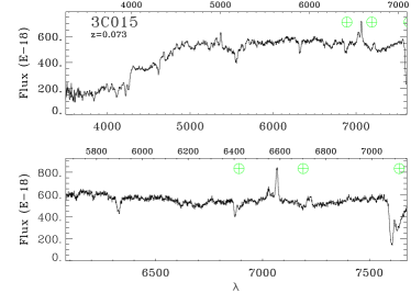
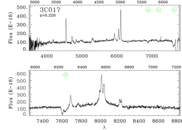
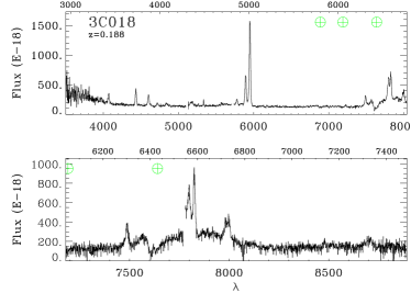
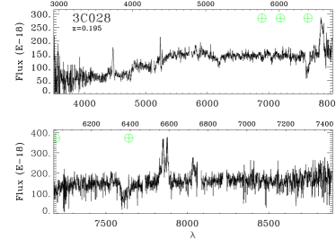
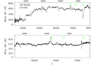
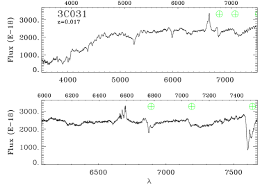
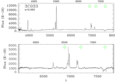
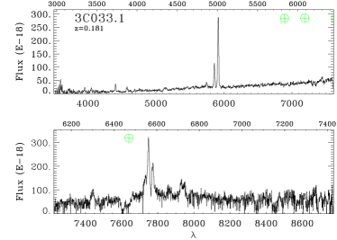
Figure 1: For each source the low (upper panels) and high resolution (bottom panels) spectra are shown. The fluxes are in units of erg cm^-2 s^-1 Å^-1 while the wavelengths are in Å. The lower axes of the spectra show the observed wavelengths while the upper axes show the rest frame wavelengths. The three main telluric absorption bands are indicated with circled crosses. For the SDSS spectra we report the whole spectrum in the upper panel and a zoom of $\sim$ 2000 Å around the H$\alpha$ line in the bottom panel. The remaining spectra are available as gif files.

(Martel et al., 1999; de Koff et al., 1996). The procedure used for the comparison is the following: we smoothed the HST image to the seeing measured in the acquisition TNG image, extracted a region corresponding to 2$\arcsec$x 2$\arcsec$, and measured its flux based on the HST absolute flux calibration. We convolved the LR-B TNG spectra with the filter transmission used to obtain the HST images (the broad band F702W filter of the Wide Field Planetary Camera 2) and measured the flux within this spectral band. We compared these two measurements and found an agreement within $\sim$ 20%. The absolute flux calibration of high resolution spectra was obtained scaling them to the low resolution calibrated spectra.

The telluric absorption bands were usually left uncorrected except in the few cases in which an emission line of interest fell into these bands. In these cases we corrected the atmospheric absorptions using the associated standard stars as templates.

Spectra for 18 3CR objects are available from the Sloan Digital Sky Survey (SDSS) database (York et al., 2000; Stoughton et al., 2002; Yip et al., 2004), Data Release 4,5,6. Since they have comparable signal to noise, resolution and wavelength coverage (3800-9200 Å) of the TNG spectra, we decided not to observe them at the TNG and to use the SDSS spectra for our analysis.

Fig. 1 shows, for all the observed targets, the low resolution spectrum (upper image) and the high resolution one (bottom image). The calibrated spectra are in units of $10^{-18}$ erg cm^-2 s^-1 Å^-1. The wavelengths (in Å units) are in the observer frame in the axes below the images while they are in the source frame in the axes above them. The three main telluric absorption bands are indicated as circles with a cross inside.

3 Data analysis

3.1 Starlight subtraction

The extraction apertures contain, in addition to the emission produced by the active nucleus, a substantial contribution from the host galaxy starlight. In order to proceed in our analysis it is necessary to separate these two components by modeling the stellar emission.

In order to prepare the spectra for the stellar removal, we corrected for reddening due to the Galaxy (Burstein & Heiles, 1982, 1984) using the extinction law of Cardelli et al. (1989). The galactic extinction E(B-V) used for each object was taken from the NASA Extragalactic Database (NED) database and is listed in Table LABEL:bigtable. We also deredshifted the spectra using the value of redshift from NED.

The spectra modeling was done considering two wavelength ranges of $\sim 1000$ Å centered on the H$\alpha$ line from the HR spectrum and on the H$\beta$ line from the LR-B spectrum. For each of the two ranges we subtracted the best fit single stellar population (SSP) model taken from the Bruzual & Charlot (2003) library. We selected a grid of 33 single stellar population models varying over 11 values of stellar ages (0.1, 0.3, 0.5, 1, 2, 3, 5, 7, 9, 11, 13 Gyr) and three values of absolute metalicity (0.008, 0.02, 0.05), see Table 2. The templates assume a Salpeter Initial Mass Function (IMF) formed in an instantaneous burst, with stars in the mass range $0.1\leq M\leq 125$ M_⊙. The parameters free to vary independently of each other in order to obtain the best fit are the stellar age, the metalicity, the normalization of the model, the velocity dispersion (line-broadening function), and a small adjustment to the published redshift. We allowed for different models for the population in the H$\beta$ and H$\alpha$ regions. In fact, as discussed in Sect. 3.3, the stellar content of radio galaxies is often composed by populations of various ages and thence the dominant population can vary in different bands. We excluded from the fit the spectral regions corresponding to emission lines, as well as other regions affected by telluric absorption, cosmic rays or other impurities. The SSP subtracted from the spectra are listed in Table 5: for each source the best fit SSP and the $\chi^{2}_{r}$ are reported for the two wavelength regions around H$\alpha$ and H$\beta$.

Table 5: Summary of the Single Stellar Population fitting.

Name	H$\beta$		H$\alpha$		Name	H$\beta$		H$\alpha$
	SSP	$\chi^{2}_{\rm r}$	SSP	$\chi^{2}_{\rm r}$		SSP	$\chi^{2}_{\rm r}$	SSP	$\chi^{2}_{\rm r}$
3C 015	16	6.29	27	1.72	3C 264	29	12.43	22	2.29
3C 017	8	2.22	33	1.63	3C 270	31	2.41	22	3.41
3C 018	28	0.81	10	1.12	3C 272.1	32	7.88	22	2.60
3C 028	29	1.04	11	0.88	3C 274	27	23.84	27	1.09
3C 029	28	2.21	28	1.53	3C 277.3	31	1.70	22	0.90
3C 031	28	4.50	28	1.43	3C 284	26	1.28	15	1.50
3C 033	7	1.43	29	0.92	3C 285	22	1.49	22	1.69
3C 035	30	1.76	22	0.89	3C 287.1	8	1.21	10	1.51
3C 040	28	7.03	28	2.52	3C 293	21	1.26	33	1.19
3C 052	29	0.90	33	1.00	3C 296	31	3.84	22	2.54
3C 061.1	18	0.83	33	0.99	3C 300	11	0.64	33	1.60
3C 066	28	4.23	28	2.31	3C 303	16	1.53	27	1.02
3C 075	32	1.93	22	2.94	3C 303.1	6	0.83	27	1.04
3C 076.1	30	2.50	11	1.29	3C 305	10	2.15	22	1.39
3C 078	32	1.18	11	0.78	3C 310	29	1.34	28	2.09
3C 079	7	1.83	10	1.10	3C 314.1	30	0.90	22	0.81
3C 083.1	32	4.19	33	7.56	3C 315	11	1.49	22	1.13
3C 088	31	1.63	32	1.08	3C 317	31	2.68	22	1.68
3C 089	30	1.77	22	0.88	3C 318.1	31	2.47	22	1.13
3C 093.1	19	1.00	32	0.95	3C 319	8	1.45	33	0.96
3C 098	26	1.91	27	2.18	3C 321	29	1.51	11	0.91
3C 105	31	0.86	33	1.12	3C 326	31	1.16	22	1.08
3C 123	33	1.98	33	3.07	3C 327	30	1.77	33	1.74
3C 129	33	0.69	33	0.98	3C 338	31	5.54	22	1.35
3C 129.1	32	0.88	32	0.68	3C 348	29	0.92	21	0.86
3C 130	32	0.82	22	0.64	3C 353	33	2.06	22	1.28
3C 133	18	0.87	10	0.97	3C 357	28	1.38	28	1.07
3C 135	29	0.95	11	1.07	3C 379.1	22	1.11	22	0.96
3C 136.1	32	1.18	32	1.22	3C 381	8	2.92	29	0.63
3C 153	31	0.95	22	1.52	3C 386	3	2.04	25	1.35
3C 165	31	0.71	10	1.92	3C 388	29	2.79	31	3.05
3C 166	18	0.95	33	1.00	3C 401	28	1.31	16	0.75
3C 171	17	0.85	20	1.13	3C 402	17	2.13	28	1.36
3C 173.1	27	0.83	16	0.75	3C 403	29	1.26	29	1.99
3C 180	8	0.83	21	0.92	3C 424	30	1.52	31	0.63
3C 184.1	30	1.92	22	1.31	3C 430	28	1.02	18	1.08
3C 192	30	1.65	22	1.14	3C 433	29	2.04	31	1.54
3C 196.1	27	0.85	6	1.33	3C 436	30	0.74	28	1.32
3C 197.1	10	1.91	20	1.89	3C 438	26	0.84	24	1.06
3C 198	16	1.42	7	1.36	3C 442	30	7.43	22	1.09
3C 213.1	17	0.76	7	0.99	3C 449	27	9.70	28	1.29
3C 219	7	1.75	20	1.47	3C 452	31	2.24	22	0.98
3C 223	20	1.59	29	0.95	3C 456	15	1.43	26	1.07
3C 223.1	30	1.54	22	1.33	3C 459	14	0.81	27	1.12
3C 236	31	1.40	22	1.05	3C 460	29	0.89	33	0.98
3C 258	2	1.63	1	0.87	3C 465	31	2.20	22	1.79

Legenda for the SSP code.

Age (Gyr)	0.1	0.3	0.5	1	2	3	5	7	9	11	13
Z=0.008	1	2	3	4	5	6	7	8	9	10	11
Z=0.02	12	13	14	15	16	17	18	19	20	21	22
Z=0.05	23	24	25	26	27	28	29	30	31	32	33

In Fig. 2 we show a few examples of the process of removal of the galaxy starlight. The six spectra presented are representative of the different quality in the sample (in order of decreasing signal-to-noise ratio from top to bottom). We show separately galaxies with different levels of line equivalent widths (high EW in the right two columns, low EW in the left 2 columns).

In a few galaxies the continuum is essentially featureless (see for example, 3C 084 in Fig. 1) and it is likely to be dominated by non-stellar emission. No starlight subtraction was performed for these objects. In several spectra a first attempt to model the starlight left substantial positive residuals in the region surrounding the H$\beta$ and/or H$\alpha$ lines, indicative of the presence of a broad line component. In these cases we flagged a spectral region extending over between 100 and 200 Å around the broad line, extended the spectral range considered, and repeated the fitting procedure (see Fig. 3 for an example).

For a few objects, we used a different technique to remove the galactic emission because we did not find a satisfactory fit using the template models. We then used as template the spectra extracted from two off-nuclear regions, flanking the nuclear aperture, summed over a spatial aperture of 2$\arcsec$ and appropriately scaled to match the nuclear spectrum. An example of this method is given in Fig. 4. The objects in which one of these different approaches was adopted are marked appropriately in Table 4.

The case of 3C 386 deserves a special note. Lynds (1971) reports that the peculiar observational characteristics of 3C 386 result from the chance superposition of a F7 star on the galaxy’s nucleus. This is confirmed by our spectra that show strong Balmer absorption lines at zero

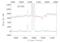
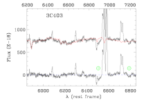
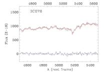
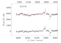
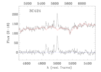
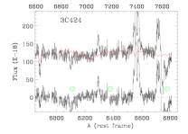
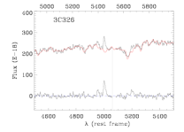
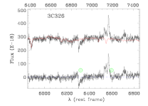
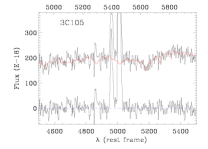
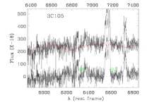
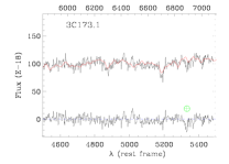
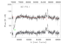
Figure 2: Examples of the process of removal of the galaxies’ starlight. The six galaxies presented are representative of the different quality in the sample (in order of decreasing signal-to-noise ratio from top to bottom) and of different levels of line equivalent widths (high EW in the left two columns, low EW in the right two columns). The original spectrum is the upper solid black line; the best fit Single Stellar Population (SSP) model is in red; the lower solid black line is the residual spectrum after SSP subtraction; the dashed blue line is a reference zero level. The flux is measured in $10^{-18}$ erg cm^-2 s^-1 Å^-1 while the wavelength is in Å, in rest frame in the lower axes and in observed frame in the axes above.

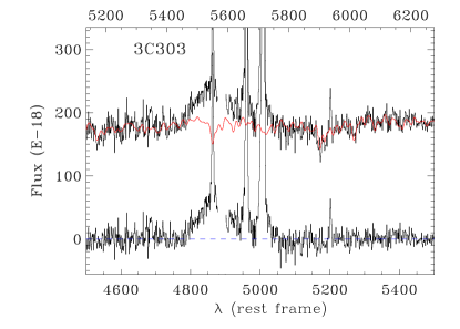
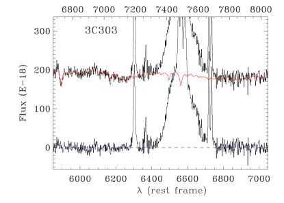
Figure 3: 3C 303: example of starlight removal for a radio galaxy with prominent broad line emission. For the line legend see Fig.2.

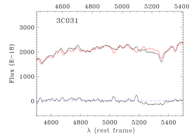
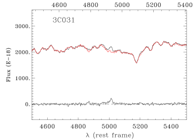
Figure 4: 3C 031: example of starlight subtraction using the off-nuclear galactic emission as template. We compare the results obtained from the standard modeling technique (left panel) and from the off-nuclear subtraction (right panel). In the latter case, the residuals have a lower amplitude and show the presence of the H$\beta$ and [O III] lines. For the line legend see Fig.2.

redshift accompanied by absorption and emission features at the redshift of the radio galaxy, z=0.0177 (see Fig. 5).

Before modeling the stellar population of this galaxy, we removed the contribution of the foreground star. We obtain the best match of the absorption lines of the star using a F5V stellar template (from Pickles 1998), with the same reddening of the galaxy, E(B-V)= 0.335. The low resolution spectrum resulting from subtracting the foreground star is shown in Fig. 5 where we also present the H$\alpha$ spectral region from the high resolution spectrum, with a well visible H$\alpha$+[N II] triplet and [S II] doublet. No broad H$\alpha$ line is visible in this spectrum in contrast to the result of Simpson et al. (1996).

3.2 Measurement of the emission lines fluxes

The next step of our analysis consists of the measurement of the emission line intensities for which we used the specfit package in IRAF. We measured line intensities fitting Gaussian profiles to H$\beta$, [O III]$\lambda\lambda$4959,5007, [O I]$\lambda\lambda$6300,64, H$\alpha$, [N II]$\lambda\lambda$6548,84, and [S II]$\lambda\lambda$6716,31. Some constraints were adopted to reduce the number of free parameters: we required the FWHM and the velocity to be the same for all the lines. The integrated fluxes of each line were free to vary except for those with known ratios from atomic physics: i.e. the [O I]$\lambda\lambda$6300,64, [O III]$\lambda\lambda$4959,5007 and [N II]$\lambda\lambda$6548,84 doublets. Where required, we insert a linear continuum.

Table LABEL:bigtable summarizes the intensities of the main emission lines (dereddened for Galactic absorption) relative to the intensity of the narrow component of H$\alpha$, for which we give flux and luminosity. To each line we associated its relative error, as a percentage. We placed upper limits at a 3$\sigma$ level to the undetected, but diagnostically important, emission lines by measuring the noise level in the regions surrounding the expected positions of the lines, and adopting as line width the instrumental resolution. When no emission lines are visible, we only report the upper limit for H$\alpha$. The missing values in Table LABEL:bigtable correspond to lines outside the coverage of the spectra or severely affected by telluric bands.

For the galaxies with a broad-line component we first attempted to reproduce the BLR emission with a gaussian profile, allowing for velocity shifts with respect to the narrow lines and also for line asymmetry. Most line profiles were well reproduced, but in some cases (e.g. 3C 332) two gaussians had to be included. Nonetheless, in 3C 111 and in 3C 445 the broad line profile is so complex, and the prominence of the broad component with respect to narrow lines is so large, it precludes any attempt to measure the [N II] doublet and the narrow component of H$\alpha$ (or H$\beta$ in the blue region of the spectrum). For these objects we use the [O III] line as reference instead of the narrow H$\alpha$ component. No narrow lines are visible in 3C 273 and we only report its broad H$\alpha$ flux. For all 18 galaxies with a broad H$\alpha$ component we also give its flux in Table LABEL:bigtable. These objects will be discussed in more detail in Sect. 4.3.

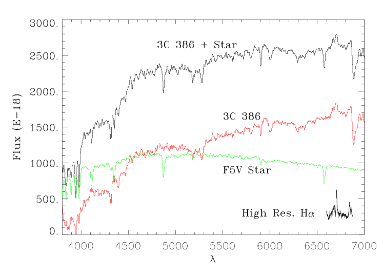
Figure 5: The case of 3C 386: a Galactic star superposed on the radio galaxy nucleus. We show the low resolution spectrum, the F5V stellar template adopted, and the resulting spectrum of the galaxy. In the bottom right corner we show also the spectrum of 3C 386 around the H$\alpha$ line obtained from the high resolution data (vertically offset for clarity).

3.3 On the effects of template mis-match on the emission lines fluxes

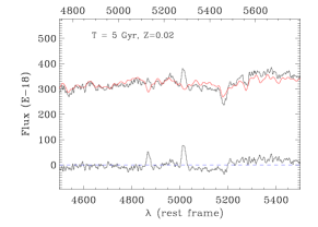
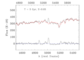
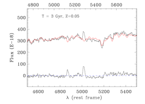
Figure 6: Example of starlight removal using models differing by one step in stellar age or in metalicity. The center panel shows the best fit for 3C 310, while the two flanking figures have (left) lower metalicity and (right) younger stellar population.

An important issue related to the subtraction of the stellar component is the effect of the template mis-match for the measurements of the emission lines. This is particularly important for the estimate of H$\beta$ in the galaxies showing emission lines of relatively low equivalent width. In fact they can be strongly affected by the level of the absorption features associated to the stellar population.

We consider as an example the case of 3C 310. Its spectrum is of average quality in our dataset and it shows only weak emission lines, while the H$\beta$ line is, at most, marginally detected in its spectrum. The best fitting stellar population has an age of 5 Gyr and a metalicity of Z=0.05 and it is shown in red in the middle panel of Fig. 6 superposed on the original spectrum. In the residual spectrum a well defined H$\beta$ line emerges in emission, caused by the removal of a substantial absorption associated with the stellar emission. This indicates that its intensity is strongly influenced by the choice of the stellar template. To associate a proper error to this procedure it is necessary to establish the range of acceptable stellar models (in terms of age and metalicity) and the resulting uncertainty in the line measurement.

As a formal error propagation across all steps of the data reduction is clearly unfeasible, we estimated the typical error of our spectra by measuring the rms flux in continuum dominated spectral regions. Even with this approach, the value of minimum reduced $\chi^{2}_{\rm r}$ obtained from the best fitting stellar population is often larger than the value indicative of a good fit ($\chi^{2}_{\rm r}\sim 1$) and this is in contrast with the fact that the stellar models seem to trace in general the spectra rather well. There are several reasons for this discrepancy: i) the $\chi^{2}_{\rm r}$ is not properly normalized (e.g. because not all data points are independent) ii) our estimate of the signal-to-noise ratio does not include the uncertainties in e.g. the wavelength and flux calibration, iii) there are real mismatches between data and models, in part caused by the use of a discrete grid of stellar models. We then decided, when necessary, to rescale our error bars such that the overall best fitting model provides $\chi^{2}$/d.o.f. = 1, following the approach proposed by Barth et al. (2001) in a different context. This is a conservative approach since it has the effect of increasing the range of the acceptable templates with respect to what would have been obtained only using the measured rms of each spectrum.

Table 6: Emission line measurements.

Name	Redshift	E(B-V)	L(H$\alpha$)	F(H$\alpha$)	H$\beta$	[O III]$\lambda$5007	[O I]$\lambda$6364	[N II]$\lambda$6584	[S II]$\lambda$6716	[S II]$\lambda$6731	F(H$\alpha$) broad
3C 015.0	0.073	0.022	40.40	-14.70 ( 2)	0.32 (20)	1.58 ( 4)	0.29 ( 8)	2.06 ( 1)	0.32 ( 8)	0.41 ( 8)
3C 017.0	0.220	0.023	41.88	-14.27 ( 1)	0.24 ( 8)	1.28 ( 1)	0.44 ( 1)	0.70 ( 1)	0.23 ( 1)	0.21 ( 2)	-13.87
3C 018.0	0.188	0.158	41.93	-14.06 ( 1)	0.33 ( 1)	4.17 ( 1)	0.43 ( 3)	1.13 ( 1)	0.38 ( 2)	0.42 ( 1)	-13.03
3C 028.0	0.195	0.058	41.51	-14.52 ( 2)	0.53 (15)	0.28 (20)	0.17 (10)	0.92 ( 3)	0.55 (10)	–
3C 029.0	0.045	0.036	40.06	-14.60 ( 6)	0.24 (25)	1.07 ( 2)	0.19 (16)	1.85 ( 1)	0.50 ( 6)	0.52 ( 4)
3C 031.0	0.017	0.001	39.83	-13.96 ( 1)	0.15 ( 8)	0.43 ( 2)	0.14 (12)	0.99 ( 1)	0.37 ( 1)	0.32 ( 1)
3C 033.0	0.060	0.028	41.63	-13.29 ( 1)	0.31 ( 1)	3.55 ( 1)	0.25 ( 1)	0.63 ( 1)	0.39 ( 1)	0.33 ( 1)
3C 033.1	0.181	0.633	41.85	-14.11 ( 1)	0.22 ( 5)	2.80 ( 1)	0.25 ( 1)	0.57 ( 1)	0.27 ( 1)	0.21 ( 1)	-13.26
3C 035.0	0.067	0.141	40.22	-14.81 ( 1)	$<$ 1.27	0.62 (23)	0.46 ( 5)	0.77 ( 2)	0.62 (15)	–
3C 040.0	0.019	0.041	39.08	-14.79 (11)	0.32 (32)	1.38 ( 6)	0.24 (28)	2.32 ( 1)	0.81 (10)	$<$ 0.52
3C 052.0	0.285	0.232	$<$ 40.64	$<$ -15.76	–	–	–	–	–	–
3C 061.1	0.184	0.176	42.05	-13.92 ( 1)	0.25 ( 4)	2.63 ( 1)	0.08 (10)	0.31 ( 1)	0.16 ( 1)	0.15 ( 3)
3C 066B	0.022	0.080	40.11	-13.90 ( 4)	0.22 ( 7)	0.87 ( 1)	0.26 (16)	2.45 ( 1)	0.56 ( 9)	–
3C 075N	0.023	0.180	39.58	-14.50 ( 1)	$<$ 2.20	$<$ 2.20	0.42 ( 2)	2.48( 1)	$<$ 0.69	0.37 ( 1)
3C 076.1	0.033	0.138	39.89	-14.50 ( 2)	$<$ 0.85	$<$ 0.92	$<$ 0.18	1.57 ( 1)	0.33 ( 4)	0.54 ( 1)
3C 078.0	0.029	0.173	39.73	-14.53 ( 3)	0.18 (30)	0.48 (16)	0.18 (13)	1.88 ( 2)	–	–
3C 079.0	0.256	0.127	42.39	-13.91 ( 1)	0.29 ( 3)	2.97 ( 1)	0.05 ( 2)	0.32 ( 1)	0.12 ( 3)	0.11 ( 7)
3C 083.1	0.027	0.164	39.40	-14.83 (14)	$<$ 0.72	$<$ 1.25	–	1.35 ( 3)	–	–
3C 084.0	0.018	0.163	41.28	-12.55 ( 1)	0.42 ( 1)	2.09 ( 1)	0.64 ( 1)	1.12 ( 1)	0.54 ( 1)	0.51 ( 1)
3C 088.0	0.030	0.126	39.98	-14.33 ( 1)	0.29 (11)	1.44 ( 2)	0.50 ( 3)	2.39 ( 1)	0.97 ( 1)	0.79 ( 3)
3C 089.0	0.139	0.134	40.28	-15.42 (11)	$<$ 1.86	$<$ 1.69	$<$ 1.26	1.43 ( 7)	–	–
3C 093.1	0.243	0.389	42.35	-13.89 ( 1)	0.28 ( 4)	2.08 ( 1)	0.28 ( 3)	1.36 ( 1)	0.54 ( 1)	0.55 ( 1)
3C 098.0	0.030	0.229	40.52	-13.79 ( 1)	0.25 ( 3)	3.01 ( 1)	0.15 ( 3)	0.76 ( 1)	0.34 (10)	0.23 ( 7)
3C 105.0	0.089	0.480	40.89	-14.39 ( 3)	0.26 (28)	3.59 ( 1)	0.38 ( 5)	1.59 ( 1)	0.55 ( 4)	0.55 ( 1)
3C 111.0	0.049	1.647	42.44a	-12.28a (1)	–	1.00a( 1)	0.04a (10)	–	0.03a ( 7)	0.03a ( 9 )	-11.64
3C 123.0	0.218	0.981	41.96	-14.18 ( 1)	0.61 (32)	1.09 (18)	0.25 (32)	2.34 ( 1)	0.48 ( 1)	0.35 ( 1)
3C 129.0	0.022	1.058	39.81	-14.20 ( 1)	$<$ 0.99	$<$ 1.10	0.61 ( 1)	1.51 ( 1)	0.50 ( 1)	0.50 (20)
3C 129.1	0.022	1.131	$<$ 39.83	$<$ -14.21	–	–	–	–	–	–
3C 130.0	0.032	1.309	$<$ 40.17	$<$ -14.19	–	–	–	–	–	–
3C 133.0	0.278	0.949	42.41	-13.97 ( 1)	0.32 ( 1)	2.26 ( 1)	0.25 ( 9)	0.70 ( 1)	0.17 ( 1)	0.14 ( 1)
3C 135.0	0.125	0.115	41.52	-14.09 ( 1)	0.33 ( 3)	3.40 ( 1)	0.18 ( 2)	0.80 ( 1)	0.30 ( 1)	0.30 ( 3)
3C 136.1	0.064	0.762	41.41	-13.57 ( 1)	0.14 ( 1)	1.08 ( 1)	0.05 ( 1)	0.59 ( 1)	0.20 ( 1)	0.20 ( 3)
3C 153.0	0.277	0.162	41.60	-14.77 ( 3)	0.23 (15)	1.07 ( 3)	0.36 ( 7)	1.21 ( 3)	0.54 ( 8)	0.33 (13)
3C 165.0	0.296	0.174	41.44	-15.00 (15)	0.44 (15)	1.68 ( 4)	0.31 (32)	1.14 (27)	0.32 (27)	0.33 (27)
3C 166.0	0.245	0.211	41.51	-14.75 ( 3)	0.42 ( 6)	1.40 ( 2)	0.38 ( 7)	0.73 ( 4)	0.41 (16)	0.34 (24)
3C 171.0	0.238	0.054	42.45	-13.78 ( 1)	0.36 ( 1)	2.73 ( 1)	0.24 ( 2)	0.57 ( 1)	0.38 ( 6)	0.29 ( 2)
3C 173.1	0.292	0.044	41.05	-15.38 ( 7)	$<$ 0.23	0.63 (12)	0.24 (28)	2.04 ( 3)	0.24 (29)	0.31 (24)
3C 180.0	0.220	0.098	41.79	-14.36 ( 1)	0.25 ( 4)	3.53 ( 1)	0.10 (28)	0.69 ( 1)	0.28 ( 3)	0.19 ( 5)
3C 184.1	0.118	0.032	41.79	-13.77 ( 3)	0.29 ( 4)	2.71 ( 1)	0.08 ( 7)	0.27 ( 8)	0.11 ( 1)	0.09 ( 3)	-13.99
3C 192.0	0.060	0.054	40.95	-13.97 ( 1)	0.30 ( 1)	2.48 ( 1)	0.11 ( 3)	0.71 ( 1)	0.35 ( 1)	0.26 ( 1)
3C 196.1	0.198	0.065	41.56	-14.48 ( 2)	0.22 (10)	0.91 ( 3)	0.20 (15)	1.19 ( 1)	0.52 ( 1)	0.49 ( 1)
3C 197.1	0.128	0.041	40.69	-14.93 ( 3)	0.37 (11)	1.69 ( 2)	0.33 ( 8)	0.76 ( 4)	0.29 (11)	0.31 ( 9)	-13.95
3C 198.0	0.082	0.026	41.31	-13.89 ( 1)	0.27 ( 1)	0.46 ( 1)	0.05 ( 9)	0.28 ( 1)	–	–
3C 213.1	0.194	0.028	41.01	-15.02 ( 3)	0.21 (14)	1.13 ( 3)	0.46 ( 6)	1.41 ( 2)	0.38 (10)	0.28 (12)
3C 219.0	0.175	0.018	41.55	-14.38 ( 2)	0.25 (10)	1.67 ( 1)	0.44 ( 3)	0.90 ( 1)	0.24 ( 6)	0.24 ( 7)	-13.87
3C 223.0	0.137	0.012	41.68	-14.01 ( 1)	0.23 ( 5)	3.09 ( 1)	0.19 ( 3)	0.63 ( 1)	0.25 ( 3)	0.21 ( 3)
3C 223.1	0.107	0.017	41.16	-14.30 ( 1)	0.28 ( 7)	2.63 ( 1)	0.06 (15)	0.81 ( 1)	0.22 ( 4)	0.19 ( 5)
3C 227.0	0.086	0.026	41.08	-14.17 ( 2)	0.44 ( 1)	4.73 ( 1)	0.08 (18)	0.19 ( 4)	0.16 ( 5)	0.16 (11)	-12.52
3C 234.0	0.185	0.019	42.64	-13.33 ( 1)	0.25 ( 2)	2.96 ( 1)	0.04 ( 8)	0.28 ( 1)	0.08 ( 3)	0.07 ( 1)	-13.29
3C 236.0	0.099	0.011	41.13	-14.25 ( 1)	0.22 ( 4)	0.57 ( 2)	0.30 ( 3)	0.69 ( 1)	0.49 ( 2)	0.35 ( 3)
3C 258.0	0.165	0.020	40.96	-14.90 (23)	0.11 (24)	0.17 (15)	$<$ 0.47	$<$ 2.14	–	–
3C 264.0	0.022	0.023	39.68	-14.35 ( 1)	0.27 ( 7)	0.33 (10)	0.22 ( 9)	1.45 ( 1)	0.33 ( 8)	0.33 (22)
3C 270.0	0.007	0.018	38.13	-14.93 ( 7)	$<$ 1.09	0.63 (25)	0.52 (16)	0.72 (14)	$<$ 0.37	$<$ 0.53
3C 272.1	0.004	0.040	38.92	-13.57 ( 1)	0.10 ( 3)	0.19 ( 4)	0.23 ( 6)	1.28 ( 1)	0.52 ( 1)	0.34 ( 1)
3C 273.0	0.158	0.021	–	–	–	–	–	–	–	–	-11.51
3C 274.0	0.004	0.022	39.50	-13.11 ( 1)	0.17 ( 1)	0.31 ( 1)	0.36 ( 1)	2.32 ( 1)	0.68 ( 1)	0.77 ( 1)
3C 277.3	0.086	0.012	40.83	-14.43 ( 1)	0.19 ( 9)	1.29 ( 1)	0.29 ( 5)	0.79 ( 3)	0.32 ( 1)	0.28 ( 5)
3C 284.0	0.239	0.016	41.41	-14.82 ( 7)	0.20 (12)	1.52 ( 1)	$<$ 0.24	0.61 (11)	$<$ 0.45	$<$ 0.41
3C 285.0	0.079	0.017	40.66	-14.52 ( 1)	0.19 ( 6)	0.78 ( 1)	0.10 (10)	0.54 ( 2)	0.27 ( 4)	0.19 ( 6)
3C 287.1	0.216	0.025	41.50	-14.62 ( 3)	0.27 ( 9)	1.71 ( 1)	0.48 ( 4)	0.68 ( 4)	0.29 ( 7)	0.29 ( 7)	-13.85
3C 293.0	0.045	0.017	40.18	-14.49 ( 3)	0.19 (17)	0.42 (10)	0.26 ( 3)	0.88 ( 1)	0.66 ( 2)	0.66 (10)
3C 296.0	0.025	0.025	39.87	-14.28 ( 1)	0.30 (12)	0.81 ( 2)	0.22 (23)	1.84 ( 1)	0.43 ( 2)	0.38 (10)
3C 300.0	0.272	0.035	41.78	-14.58 ( 2)	0.25 ( 9)	1.71 ( 1)	0.15 (13)	0.48 ( 4)	0.33 ( 4)	0.23 ( 4)
3C 303.0	0.141	0.019	41.33	-14.39 ( 1)	0.35 ( 4)	2.55 ( 1)	0.41 ( 2)	1.06 ( 1)	0.46 ( 2)	0.39 ( 3)	-13.46
3C 303.1	0.269	0.036	42.10	-14.24 ( 1)	0.26 ( 2)	2.07 ( 1)	0.24 ( 3)	1.03 ( 1)	0.38 ( 2)	0.48 ( 1)
3C 305.0	0.042	0.026	40.92	-13.68 ( 1)	0.12 ( 4)	1.30 ( 1)	0.17 ( 7)	1.77 ( 1)	0.48 ( 1)	0.40 ( 1)
3C 310.0	0.054	0.042	40.32	-14.50 ( 1)	0.23 ( 7)	0.54 ( 3)	0.30 ( 4)	1.74 ( 1)	0.84 ( 1)	0.74 ( 2)
3C 314.1	0.120	0.020	40.31	-15.25 ( 4)	0.37 (16)	0.24 (24)	0.18 (23)	0.53 ( 7)	0.52 ( 8)	0.33 (13)
3C 315.0	0.108	0.062	41.15	-14.32 ( 1)	0.20 ( 4)	0.53 ( 1)	0.25 ( 2)	0.72 ( 1)	0.51 ( 1)	0.37 ( 2)
3C 317.0	0.034	0.037	40.35	-14.08 ( 1)	0.30 ( 5)	1.00 ( 2)	0.25 ( 5)	1.92 ( 1)	0.58 ( 1)	0.49 ( 1)
3C 318.1	0.044	0.035	39.95	-14.70 ( 4)	$<$ 0.58	0.26 (32)	0.21 (19)	1.02 ( 3)	0.29 ( 9)	0.16 (13)
3C 319.0	0.189	0.012	41.16	-14.84 ( 7)	$<$ 0.13	$<$ 0.10	$<$ 0.27	0.30 ( 6)	0.15 (25)	$<$ 0.14
3C 321.0	0.097	0.044	40.50	-14.87 ( 2)	0.30 (11)	2.58 ( 1)	0.06 (28)	0.50 ( 3)	0.18 ( 8)	0.15 (11)
3C 323.1	0.264	0.042	42.21	-14.12 ( 1)	0.26 (11)	3.93 ( 1)	0.20 (11)	0.29 (32)	0.10 (11)	0.08 (21)	-12.37
3C 326.0	0.090	0.053	40.28	-15.02 ( 5)	$<$ 0.23	1.31 ( 4)	0.37 (13)	1.93 ( 3)	0.41 (12)	0.50 (11)
3C 327.0	0.104	0.089	41.73	-13.70 ( 1)	0.27 ( 4)	3.20 ( 1)	0.14 ( 1)	0.73 ( 1)	0.30 ( 1)	0.24 ( 1)
3C 332.0	0.151	0.024	41.31	-14.47 ( 2)	0.28 ( 8)	3.14 ( 1)	0.21 ( 9)	0.97 ( 1)	0.37 ( 6)	0.36 ( 7)	-12.77
3C 338.0	0.032	0.012	40.25	-14.11 ( 1)	0.18 (19)	0.21 ( 6)	0.18 ( 2)	1.63 ( 1)	0.41 ( 1)	0.33 ( 1)
3C 348.0	0.154	0.094	41.29	-14.51 ( 1)	0.25 ( 5)	0.13 ( 9)	0.27 ( 5)	1.27 ( 1)	–	–
3C 353.0	0.030	0.439	40.42	-13.90 ( 1)	0.20 (17)	0.53 ( 7)	0.30 ( 2)	1.09 ( 1)	0.56 ( 1)	0.43 ( 1)
3C 357.0	0.166	0.045	40.92	-14.96 ( 3)	0.23 (16)	1.08 ( 4)	0.46 ( 7)	1.37 ( 4)	–	–
3C 371.0	0.050	0.036	40.94	-13.82 ( 1)	0.29 (10)	1.01 ( 4)	0.51 ( 2)	1.14 ( 1)	0.32 ( 3)	0.29 ( 1)
3C 379.1	0.256	0.062	41.41	-14.89 ( 6)	0.31 ( 6)	2.80 ( 1)	0.21 (19)	1.54 ( 5)	0.30 (13)	0.28 (14)
3C 381.0	0.161	0.053	41.79	-14.05 ( 1)	0.31 ( 2)	3.83 ( 1)	0.11 ( 9)	0.53 ( 1)	–	–
3C 382.0	0.058	0.070	41.39	-13.51 ( 1)	0.31 ( 1)	2.45 ( 1)	0.29 ( 1)	1.49 ( 1)	0.12 ( 8)	0.13 ( 9)	-11.61
3C 386.0	0.017	0.335	40.17	-13.63 ( 1)	$<$ 1.08	$<$ 1.08	0.10 (17)	0.57 ( 1)	0.11 ( 7)	0.08 (10)
3C 388.0	0.091	0.080	40.83	-14.47 ( 2)	0.23 (14)	0.74 ( 3)	0.26 (13)	2.33 ( 1)	0.41 ( 1)	0.37 ( 1)
3C 390.3	0.056	0.071	41.57	-13.29 ( 1)	0.32 ( 1)	3.24 ( 1)	0.27 ( 1)	0.47 ( 1)	0.10 ( 1)	0.10 ( 1)	-11.60
3C 401.0	0.201	0.059	41.01	-15.05 ( 3)	0.30 (15)	1.10 ( 5)	0.24 (16)	1.77 ( 2)	0.46 ( 9)	0.34 (14)
3C 402.0	0.024	0.121	39.08	-15.03 ( 3)	$<$ 1.95	$<$ 2.19	0.37 (13)	2.97 ( 1)	$<$ 0.44	$<$ 0.97
3C 403.0	0.059	0.187	41.20	-13.71 ( 1)	0.25 ( 3)	3.54 ( 1)	0.13 ( 3)	0.84 ( 1)	0.25 ( 1)	0.24 ( 2)
3C 424.0	0.127	0.096	41.07	-14.55 ( 1)	0.24 ( 6)	0.54 ( 3)	0.27 ( 5)	0.79 ( 1)	0.44 ( 3)	0.40 (12)
3C 430.0	0.054	0.630	40.12	-14.72 ( 3)	$<$ 1.09	1.61 ( 9)	0.33 (20)	1.43 ( 1)	0.37 ( 8)	0.40 ( 4)
3C 433.0	0.102	0.145	41.40	-14.01 ( 1)	0.19 ( 4)	1.88 ( 1)	0.22 ( 3)	1.09 ( 1)	0.46 ( 2)	0.30 ( 1)
3C 436.0	0.214	0.089	41.07	-15.06 (10)	0.20 (22)	3.09 ( 1)	–	2.08 ( 9)	0.63 (19)	0.49 (18)
3C 438.0	0.290	0.358	41.55	-14.87 ( 1)	$<$ 0.54	$<$ 0.82	$<$ 0.67	1.61 ( 1)	$<$ 0.66	0.46 (28)
3C 442.0	0.026	0.065	39.78	-14.40 ( 1)	0.08 (24)	0.27 ( 7)	0.19 ( 8)	1.84 ( 1)	0.35 ( 5)	0.45 ( 1)
3C 445.0	0.056	0.083	42.50a	-12.37a ( 1)	–	1.00a ( 1)	0.04a ( 6)	–	0.02a (10)	0.02a (10)	-12.03
3C 449.0	0.017	0.167	39.71	-14.09 ( 1)	0.10 (23)	0.30 (24)	0.13 ( 9)	1.38 ( 1)	0.29 ( 7)	0.22 ( 1)
3C 452.0	0.081	0.137	41.16	-14.05 ( 1)	0.23 ( 5)	1.53 ( 1)	0.27 ( 2)	1.08 ( 1)	0.36 ( 1)	0.29 ( 1)
3C 456.0	0.233	0.038	42.48	-13.72 ( 1)	0.32 ( 1)	2.15 ( 1)	0.15 ( 2)	0.78 ( 1)	0.22 ( 1)	0.24 ( 1)
3C 459.0	0.220	0.066	42.17	-13.97 ( 1)	0.16 ( 6)	0.73 ( 1)	0.12 ( 1)	1.77 ( 1)	0.35 ( 1)	0.33 ( 1)
3C 460.0	0.269	0.092	42.09	-14.25 ( 3)	0.25 ( 3)	0.49 ( 7)	0.39 ( 4)	1.23 ( 2)	0.60 ( 1)	0.54 ( 4)
3C 465.0	0.030	0.069	40.15	-14.17 ( 1)	0.17 (27)	0.46 ( 6)	0.26 ( 9)	2.77 ( 1)	0.47 ( 1)	0.32 ( 1)

Column description: (1) source name; (2) redshift; (3) Galactic absorption; (4) logarithm of the luminosity of the H$\alpha$ narrow line, in erg s^-1; (5) logarithm of the H$\alpha$ flux in erg cm^-2 s^-1; (6 through 11) de-reddened flux ratios of the key diagnostic lines with respect to H$\alpha$. The values in parentheses report the errors (in percentage) of each line. Missing values marked with ‘–’ correspond to lines outside the coverage of the spectra or severely affected by telluric bands. When no lines are visible we only give the upper limit for H$\alpha$; (12) logarithm of the flux of the H$\alpha$ broad component, when visible.
Notes: (a) for 3C 111 and 3C 445, no narrow H$\alpha$ measurement is possible and we give instead the [O III] luminosity, referring the flux ratios to this line. No narrow lines are visible in 3C 273 and we only report its broad H$\alpha$ flux.

We consider as acceptable templates all stellar populations for which the resulting $\chi^{2}$ is increased by less than $\Delta\chi^{2}$ = 9.21, corresponding to a confidence level of 99% ($\sim$ 2.6 $\sigma$ level) for 2 parameters. In the case of 3C 310, the error derived setting $\chi^{2}_{\rm r}=1$ is 9.5 $10^{-18}$ erg cm^-2 s^-1 Å^-1. This value is similar to the rms of the stellar subtracted spectrum, which is 8.2 $10^{-18}$ erg cm^-2 s^-1 Å^-1. Adopting the procedure outlined above, the best fit is the only statistically acceptable model. Nonetheless, in Fig. 6 we show the two models with the lower values of $\chi^{2}_{\rm r}$, differing by one step in metalicity or age. In both cases significant residuals already emerge in the continuum subtracted spectrum, confirming visually the poorer quality of the fit. We re-estimate the H$\beta$ flux resulting from these two templates. They differ by $\sim$ 4% with respect to our original measurement using the best fit model. This is lower than the statistical error associated by specfit to this measurement, which is 7 %. We conclude that, in the case of 3C 310, a possible template mis-match does not have a significant effect on the H$\beta$ flux measurement.

The influence of the stellar templates on the other emission lines (and in particular on the H$\alpha$ line that is $\mathchar 13350\relax$ 3 brighter that H$\beta$ while they have the same EW in absorption) is negligible because the stellar population has not significant absorption features at the line wavelengths.

For the majority of the sources, only models differing by at most one step in age or in metalicity are consistent with the data, without a significant impact on the H$\beta$ flux. Only for the lower quality spectra can this range be broader. For low SNR spectra, coupled with emission lines of low equivalent widths, the resulting measurement error is dominated by the choice of the stellar template. In these cases we adopted the following strategy: we subtracted the acceptable template with the lowest age (i.e. with the strongest H$\beta$ absorption) and considered the H$\beta$ measurement as an upper limit. One of such galaxy is 3C 173.1, already shown in the bottom right panel of Fig. 2.

Finally we note that our approach to the starlight subtraction is limited to the choice of the best fitting single population model, similarly to the method adopted by Kauffmann et al. (2003) for the SDSS sample of emission line galaxies and by Tadhunter et al. (1993) for the 2Jy sample of radio galaxies. Nonetheless, this procedure does not grasp the complexity of the emission processes in radio galaxies. As clearly shown by several studies in the literature the stellar content of radio galaxies is often composed by populations of different ages, and there are also evidence for internal absorption, particularly associated to the young stars component (e.g. Wills et al. 2004; Raimann et al. 2005; Tadhunter et al. 2005; Holt et al. 2007). The presence of stars of various ages is indirectly confirmed by the fact that the best fit stellar population found in the H$\beta$ regions is on average $\sim$ one step in age younger than for the H$\alpha$ band. This can be explained by the higher relative contribution of young stars at shorter wavelengths that drives the age of the SSP to lower values with respect to the redder part of of the spectrum. Furthermore, other mechanisms contribute to the continuum emission, e.g. nebular continuum and light from the accretion disk (direct or via scattering). However, a full separation of these contributions requires a detailed analysis on a object-by-object basis in order to properly measure the rather large set of free parameters describing the various components. Moreover this fitting requires spectra with a high signal to noise, and this is not always achieved in our data. We defer such a study to a forthcoming paper.

There is however a general consideration that can be drawn already at this stage. Nuclear emission and nebular continuum are expected to be in general bluer that the starlight. This biases the derived age of the single stellar population that appears younger that it actually is. It also dilutes the stellar absorption features, thus biasing the metalicity to lower values. The main resulting effect is an overestimate of the correction of the H$\beta$ line and, consequently, an over-rating of this line, particularly in the objects with brightest optical nuclei.

4 Results

4.1 Emission line data quality

We summarize here the data quality of our spectra from the point of view of the measurements of the emission line intensities. Only in three radio galaxies (namely 3C 052, 3C 129.1 and 3C 130) did we fail to detect any emission line; in all cases an accurate redshift can be measured by fitting the stellar population models based on stellar absorption features.

Leaving aside these objects, the H$\alpha$ line can be measured with a statistical accuracy of better than 10 % with only three exceptions. In the red part of the spectrum, the [O I]$\lambda$6300 line is detected in 95 % of the 3C galaxies. The completeness of the [S II] doublet measurements is slightly lower (87 %) due to our choice to favor the inclusion of the [O I] in the high resolution spectra but, when covered by the data, the [S II] line is also measurable in 95 % of the objects. In the blue part of the spectrum there are $\sim$ 15 % of the sources in which H$\beta$ and/or [O III] are not detected.

All together, these measurements will enable us to locate the vast majority of the sources in the diagnostic planes that compare pairs of emission line ratios and also to perform a detailed analysis of the relationship between the multiwavelength characteristics of the 3C sources with their emission line properties.

In addition, a broad H$\alpha$ line is seen in 18 galaxies and these are discussed in more detail in the Sect. 4.3.

Figure 7: Comparison of our [O III] luminosity measurements with the values collected by Willott et al. (1999) from dishomogeneous works in literature (left panel), by Simpson et al. (1996) (center panel) and by Tadhunter et al. (1993) (right panel). The luminosities are in units of erg s^-1 while the fluxes are in units of erg s^-1 cm^-2. The solid line traces where the compared objects have the same fluxes, while the two dotted lines above and below the solid line limit the region in which the fluxes differ by less than a factor of 2. The arrows indicate the upper limits.

4.2 Comparison with previous results

There is a extremely vast amount of spectroscopic data accumulated for the 3CR sample in the literature over the last 40 years and it is therefore, on the one hand, very interesting to contrast our measurements with those available, but, on the other hand, difficult to perform a full comparison on an object-by-object basis. We therefore decided to focus on three papers, those having the largest overlap with our sample.

Willott et al. (1999) collected [O III] measurements from optical spectra and images of 3CR objects from the literature (these data are available at the web-page: http://www.science.uottawa.ca/$\sim$cwillott/3crr/3crr.html). There are 28 sources in common with our sample. Fig. 7 (left panel) shows the comparison between their data collection and our measurements, performed after scaling their reported luminosities to our cosmological parameters. These data show large discrepancies, even in excess of a factor of 100, particularly for the sources with the lowest [O III] fluxes. Sources with stronger fluxes are in better agreement with our results, but there are still large differences.

In the central and right panels we compare our [O III] fluxes with the values found by Simpson et al. (1996) and Tadhunter et al. (1993), derived from long-slit spectra of two complete samples, with respectively 8 and 16 sources in common with our 3CR subsample. Their data have been corrected for Galactic absorption before comparison. Quite reassuringly, essentially all sources have [O III] fluxes differing by less than a factor of 2.

4.3 Radio galaxies with broad emission lines

In 18 sources, all of them FR II galaxies, we detected a broad H$\alpha$ component. Broad lines can be very strong, as in 3C 273, or, as in 3C 184.1, they become clearly visible only after the subtraction of the stellar light. Fig. 8 shows all spectra showing the H$\alpha$ broad components: the dashed line, representing the continuum emission, corresponds to the zero flux level when the SSP has been subtracted, otherwise it represents the AGN power law emission.

In some cases they are symmetric and centered on the narrow component (3C 287.1), but more often they are highly red or blue shifted (3C 184.1, 3C 227). In most objects the H$\alpha$ line presents a highly irregular profile, with ‘bumps’ in the line wings. For example, in 3C 197.1 and 3C 445 the broad component has a step-shaped emission in the red wing, while in 3C 227 the step-shaped emission is on the blue side of the line. We also confirm the ‘double-humped’ shape of the BLR of 3C 332 (Eracleous & Halpern, 1994).

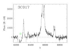
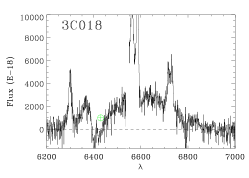
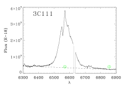
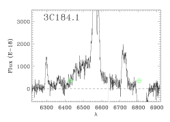
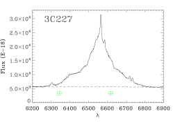
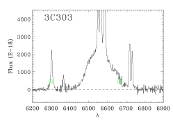
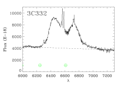
Figure 8: Radio galaxies with a broad H$\alpha$ emission line. The dashed line represents the continuum emission level. A null continuum level implies that the continuum has been removed during the process of starlight subtraction. The flux is measured in $10^{-18}$ erg cm^-2 s^-1 Å^-1 while the wavelength is in Å units.

The technique used to measure the narrow line fluxes (described in Sect. 3.2) provides us also with flux estimates for the broad components. In the cases where no satisfactory fit was obtained with multiple gaussians, we measured the flux by directly integrating the area defined by the broad component. The H$\alpha$ broad line fluxes are reported in the last column of Table LABEL:bigtable.

We will explore in more detail the issue of the presence and properties of broad lines in a forthcoming paper.

5 Summary

We presented a homogeneous and 92 % complete dataset of optical nuclear spectra of the 113 3CR radio sources with redshift $<$ 0.3. The data were obtained mostly from observations performed at the Telescopio Nazionale Galileo and are complemented with SDSS spectra, available for 18 galaxies. For each source we obtained a low (20 Å) resolution spectrum covering the $\sim$3500-8000 Å spectral range and a higher (5 Å) resolution spectrum centered on the H$\alpha$ line and $\sim$1700 Å wide. From the two dimensional calibrated data, we extracted spectra over a 2$\arcsec$ x 2$\arcsec$ nuclear region. A complete atlas of the optical nuclear spectra is presented.

We separated the contribution of the emission produced by the active nucleus from the galaxy starlight. This has been achieved by subtracting the best fit model of stellar emission from a grid of single stellar population templates. We then measured and tabulated the fluxes of the main emission lines by fitting gaussians to the residual spectra. We discussed the effects of the possible mis-match between the galaxies stellar population and the adopted templates; the conclusion of this analysis is that they do not affect significantly the line measurements, with only very few exceptions where the estimate of the H$\beta$ flux is compromised.

Only in three radio galaxies did we fail to detect any emission line. In most cases ($\sim$90 % of the sample) we were able to measure all the brightest lines, e.g. H$\beta$, [O III]$\lambda\lambda$4959,5007, [O I]$\lambda\lambda$6300,64, H$\alpha$, [N II]$\lambda\lambda$6548,84, and [S II]$\lambda\lambda$6716,31.

In addition, a broad H$\alpha$ line is seen in 18 galaxies. They show a wide variety in terms of line profiles, from well behaved symmetric lines centered onto the narrow H$\alpha$, to ‘double humped’ lines, but also include highly irregular shapes, with secondary peaks and steps.

The data presented here will be used in follow up papers to address the connection between the optical spectral characteristics and the multiwavelength properties of the sample.

Acknowledgments. We thank the referee, Katherine Inskip, for her useful comments and suggestions. SB and ACe acknowledge the Italian MIUR for financial support. ACa acknowledges COFIN-INAF-2006 grant financial support. This research has made use of the NASA/IPAC Extragalactic Database (NED) which is operated by the Jet Propulsion Laboratory. California institute of Technology, under contract with the National Aeronautics and Space Administration. This research has made use of NASA’s Astrophysics Data System (ADS). This research has made use of the SDSS Archive, funding for the creation and distribution of which was provided by the Alfred P. Sloan Foundation, the Participating Institutions, the National Aeronautics and Space Administration, the National Science Foundation, the U.S. Department of Energy, the Japanese Monbukagakusho, the Max Planck Society, and The Higher Education Funding Council for England. The official SDSS Web site is www.sdss.org. The SDSS is managed by the Astrophysical Research Consortium for the Participating Institutions. The Participating Institutions are the American Museum of Natural History, Astrophysical Institute Potsdam, University of Basel, University of Cambridge, Case Western Reserve University, University of Chicago, Drexel University, Fermilab, the Institute for Advanced Study, the Japan Participation Group, Johns Hopkins University, the Joint Institute for Nuclear Astrophysics, the Kavli Institute for Particle Astrophysics and Cosmology, the Korean Scientist Group, the Chinese Academy of Sciences (LAMOST), Los Alamos National Laboratory, the Max-Planck-Institute for Astronomy (MPIA), the Max-Planck-Institute for Astrophysics (MPA), New Mexico State University, Ohio State University, University of Pittsburgh, University of Portsmouth, Princeton University, the United States Naval Observatory, and the University of Washington.

References

- Barth et al. (2001) Barth, A. J., Sarzi, M., Rix, H., et al. 2001, ApJ, 555, 685
- Bennett (1962a) Bennett, A. S. 1962a, MNRAS, 125, 75
- Bennett (1962b) Bennett, A. S. 1962b, MmRAS, 68, 163
- Bruzual & Charlot (2003) Bruzual, G. & Charlot, S. 2003, MNRAS, 344, 1000
- Burstein & Heiles (1982) Burstein, D. & Heiles, C. 1982, AJ, 87, 1165
- Burstein & Heiles (1984) Burstein, D. & Heiles, C. 1984, ApJS, 54, 33
- Cardelli et al. (1989) Cardelli, J. A., Clayton, G. C., & Mathis, J. S. 1989, ApJ, 345, 245
- de Koff et al. (1996) de Koff, S., Baum, S. A., Sparks, W. B., et al. 1996, ApJS, 107, 621
- Edge et al. (1959) Edge, D. O., Shakeshaft, J. R., McAdam, W. B., Baldwin, J. E., & Archer, S. 1959, MmRAS, 68, 37
- Eracleous & Halpern (1994) Eracleous, M. & Halpern, J. P. 1994, ApJS, 90, 1
- Fanaroff & Riley (1974) Fanaroff, B. L. & Riley, J. M. 1974, MNRAS, 167, 31P
- Holt et al. (2007) Holt, J., Tadhunter, C. N., González Delgado, R. M., et al. 2007, MNRAS, 381, 611
- Kauffmann et al. (2003) Kauffmann, G., Heckman, T. M., White, S. D. M., et al. 2003, MNRAS, 341, 33
- Lynds (1971) Lynds, R. 1971, ApJ, 168, L87+
- Martel et al. (1999) Martel, A. R., Baum, S. A., Sparks, W. B., et al. 1999, ApJS, 122, 81
- Pickles (1998) Pickles, A. J. 1998, PASP, 110, 863
- Raimann et al. (2005) Raimann, D., Storchi-Bergmann, T., Quintana, H., Hunstead, R., & Wisotzki, L. 2005, MNRAS, 364, 1239
- Simpson et al. (1996) Simpson, C., Ward, M., Clements, D. L., & Rawlings, S. 1996, MNRAS, 281, 509
- Spinrad et al. (1985) Spinrad, H., Marr, J., Aguilar, L., & Djorgovski, S. 1985, PASP, 97, 932
- Stoughton et al. (2002) Stoughton, C., Lupton, R. H., Bernardi, M., et al. 2002, AJ, 123, 485
- Tadhunter et al. (2005) Tadhunter, C., Robinson, T. G., González Delgado, R. M., Wills, K., & Morganti, R. 2005, MNRAS, 356, 480
- Tadhunter et al. (1993) Tadhunter, C. N., Morganti, R., di Serego-Alighieri, S., Fosbury, R. A. E., & Danziger, I. J. 1993, MNRAS, 263, 999
- Willott et al. (1999) Willott, C. J., Rawlings, S., Blundell, K. M., & Lacy, M. 1999, MNRAS, 309, 1017
- Wills et al. (2004) Wills, K. A., Morganti, R., Tadhunter, C. N., Robinson, T. G., & Villar-Martin, M. 2004, MNRAS, 347, 771
- Yip et al. (2004) Yip, C. W., Connolly, A. J., Vanden Berk, D. E., et al. 2004, AJ, 128, 2603
- York et al. (2000) York, D. G., Adelman, J., Anderson, Jr., J. E., et al. 2000, AJ, 120, 1579