Stochastic Resonance phenomena in qubit arrays

Abstract

We discuss stochastic resonance–like effects in the context of coupled quantum spin systems. We focus here on an information–theoretic approach and analyze the steady state quantum correlations (entanglement) as well as the global correlations in the system when subject to different forms of local decoherence. In the presence of decay, it has been shown that the system displays quantum correlations only when the noise strength is above a certain threshold. We extend this result to the case of a Heisenberg $XYZ$ exchange interaction and revise and clarify the mechanisms underlying this behaviour. In the presence of pure dephasing, we show that the system always remains separable in the steady state. When both types of noise are present, we show that the system can still exhibit entanglement for long times, provided that the pure dephasing rate is not too large.

1 Introduction

The phenomenon of stochastic resonance (SR) benzi epitomizes the peculiar ways by which the interplay between coherent and incoherent interactions may yield an optimized system’s response, as quantified by some suitable figure of merit, for some intermediate noise strength sr98 . Initial studies on classical and semiclassical systems soon extended to the quantum domain sr98 ; andreas ; qsr ; milena ; grifoni1n ; grifoni2n , while the concept of SR itself broadened to account for an enhanced response in the presence of an optimal noise rate with bu1 ; ours ; Goychuk1 or without nancy ; bu2 ; viola an underlying synchronization effect Goychuk2 . Our interest here focuses on this latter situation with the additional ingredient that we will be dealing with interacting quantum systems carrays . In this case, the system may display not only quantum coherence but also quantum correlations (entanglement) across subsystems. The typical scenario we will be analyzing is depicted, in its simplest form, in figure 1. Two spin–1/2 particles (qubits) are coupled via a Hamiltonian interaction $V_{\mathrm{Q-Q}}$ and individually driven whilst subject to local forms of noise that we will model as independent sets of harmonic oscillators. The driving is supposed to be weak, in the sense that the external Rabi frequency $\Omega_{j}$ is constrained to be such that $\Omega_{j}\ll\omega_{0}^{j}$ and $\Omega_{j}\sim J$, where $\omega_{0}^{j}$ denotes the local spin energy and $J$ is the inter-qubit coupling strength. We will say that the system displays SR–like behaviour when we can identify some suitable figure of merit to characterize the system response in the steady state, be it dynamical or information–theoretic, such that it is nonmonotonic as a function of the environmental noise strength. Dynamical figures of merit for coupled, driven spin systems are typically magnetization properties along a given direction HP07 , which provide a suitable generalization of the standard measurements proposed for single spin systems bu1 ; nancy . Here we will focus on an information theoretic approach and adopt the quantum mutual information, which measures the total amount of correlations across any bipartition in the system Henderson , as the suitable figure of merit to quantify the presence of SR igor . Of particular interest for us is discerning whether there is steady state entanglement in the system. In the case of bipartite entanglement this will be quantified by a suitable entanglement measure like, for instance, the entanglement of formation eof (see Sect. 2 for precise definitions).

We have organized the presentation of our results as follows. We start by discussing the case of system qubits subject to pure decay. We first revise the case of longitudinally coupled qubits discussed in HP07 and revisit in some detail the basic mechanisms yielding an inseparable mixed steady state. We show that similar results hold when qubits couple via an exchange interaction, which has been the object of recent interest in the related context of noise assisted excitonic transport aspuru ; bio ; olaya ; fleming . The next section deals with systems subject to pure dephasing and we show that no steady-state correlations will be displayed in this case. Finally we analyze the case when the array is subject to both types of noise and re-evaluate the emergence of a threshold, above which quantum correlations are non zero, in this situation, as well as the behaviour of the total correlation content. The final section summarizes our findings and elaborates on future work.

2 Steady state entanglement in qubit chains subject to longitudinal decoherence (pure decay)

The system to study is a chain of $N$ coupled qubits, each of them interacting with independent, local,

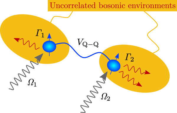
Figure 1: Illustration of the generic set up. The simplest scenario if provided by an array of $N=2$ qubit systems, whose quantum state we denote by $\rho_{12}$, with coherent interaction Hamiltonian $V_{\mathrm{Q-Q}}$ subject locally to an external driving of strength $\Omega_{j}$ and a decohering environment to which it couples with strength $\Gamma_{j}$. Note that the noise is local and therefore does not act as direct mediator of qubit interactions.

harmonic baths and driven by an external field, so the total system+environment Hamiltonian will be given by

$$H=-\frac{1}{2}\sum_{j=1}^{N}\omega^{j}_{0}\sigma_{z}^{j}+\sum_{j,k}\omega_{k}^{j}(a_{k}^{j})^{\dagger}a_{k}^{j}+\sum_{j=1}^{N}\Omega_{j}(\sigma_{+}^{j}e^{-i\omega_{L}^{j}t}+\mathrm{h.c.})+V_{\mathrm{Q-Q}}+V_{\mathrm{Q-Bath}},$$ (1)

here $V_{\mathrm{Q-Q}}$ denotes the interqubit coupling Hamiltonian and $V_{\mathrm{Q-Bath}}=\sum_{j=1}^{N}\hat{\xi}^{j}\otimes X^{j}=\sum_{j,k}C_{k}\hat{\xi}^{j}\otimes[a_{k}^{j}+(a_{k}^{j})^{\dagger}]$ is the Hamiltonian term describing the interaction with the baths. Let us consider the case first analyzed in HP07 where qubits exhibit longitudinal coupling of the form $V_{\mathrm{Q-Q}}=-J\sum_{j=1}^{N-1}\sigma_{z}^{j}\otimes\sigma_{z}^{j+1}$ and qubit–bath coupling $\hat{\xi}^{j}=\sigma_{x}^{j}$. We adopt here the notation principles when referring to transverse or longitudinal coupling and note that a longitudinal decoherence allows for energy exchange while a transverse coupling to the bath results solely in pure dephasing.

Moving to a frame rotating with the external driving (by the unitary transformation $U=\prod_{j=1}^{N}e^{i\omega_{L}^{j}\sigma_{z}^{j}}$), we arrive at the following master equation for the reduced density matrix of the qubits

$$\frac{d\rho}{dt}=-i\left(H_{\mathrm{eff}}\rho-\rho H_{\mathrm{eff}}^{\dagger}\right)+2\sum_{j=1}^{N}\Gamma_{j}(\bar{n}_{j}+1)\sigma_{-}^{j}\rho\sigma_{+}^{j}+2\sum_{i=1}^{N}\Gamma_{j}\bar{n}_{j}\sigma_{+}^{j}\rho\sigma_{-}^{j},$$ (2)

where we have introduced an effective, non-Hermitian term

$$H_{\mathrm{eff}}=H_{\mathrm{coh}}-i\sum_{j=1}^{N}\Gamma_{j}(\bar{n}_{j}+1)\sigma_{+}^{j}\sigma_{-}^{j}-i\sum_{j=1}^{N}\Gamma_{j}\bar{n}_{j}\sigma_{-}^{j}\sigma_{+}^{j},$$ (3)

with the coherent part of the evolution contained in

$$H_{\mathrm{coh}}=-\frac{1}{2}\sum_{j}\delta^{j}\sigma_{z}^{j}+\sum_{j=1}^{N}\Omega_{j}\sigma_{x}^{j}-J\sum_{j=1}^{N-1}\sigma_{z}^{j}\otimes\sigma_{z}^{j+1},$$ (4)

where $\delta^{j}$ is the detuning from the qubit transition frequency, $\Omega_{j}$ denotes the Rabi frequency of the external driving and $J$ is the strength of the coherent interqubit coupling. The number of quanta in the local baths is given according to the Bose-Einstein distribution $\bar{n}_{j}=[\exp(\omega_{0}^{j}/k_{\mathrm{B}}T)-1]^{-1}$. In addition the decay rates are expressed as $\Gamma_{j}=\pi\mathcal{J}(\omega_{0}^{j})$ where $\mathcal{J}(\omega)=\sum_{k}C_{k}^{2}\delta(\omega-\omega_{k}^{j})$ is the spectral density of each bath. This master equation treatment is valid in the parameter regime $\Omega_{j}/\omega\ll 1$, $\Gamma_{j}\bar{n}/\omega\ll 1$, $\delta_{j}/\omega\ll 1$ and $J/\omega\ll 1$, where $\omega=\min\{\omega_{0}^{j},\omega_{c}\}$ for a suitable bath’s frequency cut off $\omega_{c}$ cohen . Note that in our study, decoherence rates will be considered as ad-hoc parameters whose specific value is set by the details of the qubit–bath interaction and the noise’s spectral properties so that these parameters provides with an effective measure of the noise strength acting on the system. Moreover, we will operate at $T=0$ given that the presence of a (realistic) finite temperature does not modify the qualitative features we discuss, but simply reduces the amplitude of the entanglement or mutual information maximal values, as shown in HP07 .

Let us consider the simplest case where the arrays consist of only two qubits whose state we will denote by $\rho_{12}$, as depicted in figure 1, and let us assume, for simplicity, that $\Omega_{1}=\Omega_{2}=\Omega$ and $\Gamma_{1}=\Gamma_{2}=\Gamma$. At perfect tuning $\delta_{j}=0$ and zero temperature, the steady state of the master equation given by equation (2) can be computed analytically to be HP07

$$\rho^{\mathrm{ss}}_{12}=\frac{1}{k}\left(\begin{array}[]{cccc}t^{2}+4s^{2}r^{2},&2sr^{2}+irt,&2sr^{2}+irt,&2irs-r^{2}\\ 2sr^{2}-irt,&t,&r^{2},&ir\\ 2sr^{2}-irt,&r^{2},&t,&ir\\ -2irs-r^{2},&-ir,&-ir,&1\end{array}\right)$$ (5)

where $k=3+2r^{2}+t^{2}+4r^{2}s^{2}$, $r=\Gamma/\Omega$, $s=J/\Omega$ and $t=r^{2}+1$. This state is separable if, and only if, its partial transpose is a positive operator horo . We find that $\rho^{\mathrm{ss}}_{12}$ is entangled for values of the noise strength $\Gamma$ such that

$$\Gamma>\Gamma_{\mathrm{th}},\quad\mathrm{where}\ \Gamma_{\mathrm{th}}=\frac{\Omega^{2}}{2J}.$$ (6)

As a result, the systems exhibit quantum correlations in the steady state only if the noise strength, encapsulated in the parameter $\Gamma$, is above the threshold value $\Gamma_{\mathrm{th}}$. Otherwise, the steady state is fully separable. In order to shed light onto this rather counterintuitive behaviour, it is useful to analyze the structural form of the steady state density matrix by calculating its spectral resolution. One can easily evaluate the eigenvalues of the density matrix specifying the steady state equation (5) to be

$$\lambda_{1,2} = \frac{1}{4r^{2}s^{2}+(1+t)^{2}},$$ (7)

$$\lambda_{3,4} = \frac{1+r^{2}\left(2+4s^{2}\right)+t^{2}\mp\sqrt{4r^{2}\left(1+s^{2}\right)+(t-1)^{2}}\sqrt{4r^{2}s^{2}+(1+t)^{2}}}{2\left(4r^{2}s^{2}+(1+t)^{2}\right)}.$$ (8)

The corresponding expressions for the eigenvectors are not so compact. Figure 2 shows these eigenvalues as a function of the noise strength as well as the steady state entanglement as measured by the entanglement of formation $E_{F}(\rho_{12})$. This quantity represents the minimal possible average entanglement over all pure state decomposition of $\rho$ and as such, its evaluation requires solving a variational problem. However, in the case of two qubits, the entanglement of formation has a simple closed form in terms of the so-called two-qubit concurrence, defined as $C(\rho)=\max\{0,\mu_{1}-\mu_{2}-\mu_{3}-\mu_{4}\}$, where the $\mu_{i}$ are, in decreasing order, the eigenvalues of the matrix $\rho\sigma_{y}\otimes\sigma_{y}\rho^{\ast}\sigma_{y}\otimes\sigma_{y}$, where $\rho^{\ast}$ is the matrix obtained by element complex conjugation of $\rho$ eof . For any bipartite qubit state,

$$E_{F}(\rho)=s\left(\frac{1+\sqrt{1-C^{2}(\rho)}}{2}\right),$$ (9)

where $s(x)=-x\log_{2}x-(1-x)\log_{2}(1-x)$. We see in figure 2 that the entanglement of formation is zero for noise values below threshold, while displaying the typical SR-like profile for $\Gamma>\Gamma_{\mathrm{th}}$. When looking at the behaviour of the spectral components, we observe that as $\Gamma$ increases, the weights of some spectral components decrease and the chain tends to localize in a certain eigenstate, in this case the one corresponding to $\lambda_{4}$, which in the limit $\Gamma\rightarrow\infty$ is actually the product state of the local Hamiltonian ground states. That means the qubits tend to be in their individual ground states as the effective decay rate becomes very large, as would be expected intuitively. Interestingly, the approach to this separable steady-state, and therefore the system’s purity, is monotonic in the noise strength $\Gamma$, despite the steady-state entanglement exhibiting nonmonotonic SR–like behaviour.

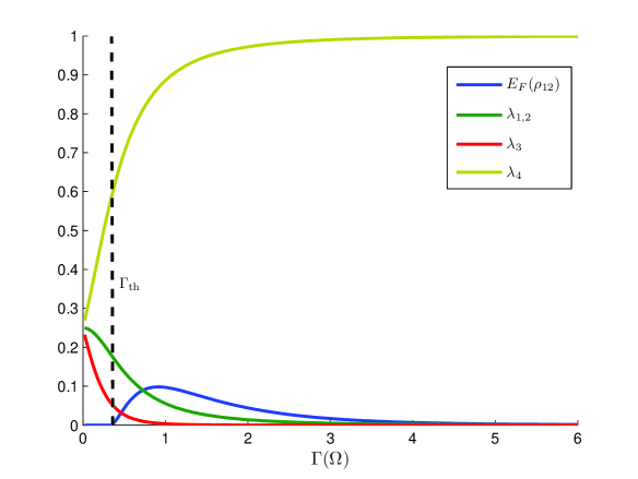
Figure 2: Eigenvalues and entanglement content of the steady state given by equation (5) as a function of the noise strength (for $J/\Omega=1.5$). The dashed vertical line divides entangled and separable regimes. See main text for explanations.

This picture is in agreement with the behaviour already described in plenio02 where, in the absence of dissipative noise in the form of an additional heat bath, a thermally driven composite system would approach a thermal steady state, while the presence of a second heat bath at different temperature has the potential to make the steady state mixture entangled. This behaviour may in fact be quite general as closely related scenarios have now been identified where steady state entanglement in facilitated by the presence of a noisy channel hans ; brandes ; aguado .

3 XXYY Heisenberg Interaction

It is worth exploring whether these results remain valid for other kinds of qubit–qubit interactions. The most general coupling between qubits is given by the Heisenberg Hamiltonian

$$V_{\mathrm{Hei}}=-J_{x}\sigma_{x}\otimes\sigma_{x}-J_{y}\sigma_{y}\otimes\sigma_{y}-J_{z}\sigma_{z}\otimes\sigma_{z}.$$

However, the evolution equation for this general Hamiltonian can no longer be written in terms of a time independent effective Hamiltonian, because the transformation $U=\prod_{j=1}^{N}e^{i\omega_{L}^{j}\sigma_{z}^{j}}$ does not commute with $V_{XXYY}$. As long as the frequency of the driving is the same for each qubit $\omega_{L}^{j}=\omega_{L}$, the most general Heisenberg-type of Hamiltonian which is time–independent in the rotating picture is the so-called XXYY interaction:

$$V_{\mathrm{XXYY}}=-J_{\perp}(\sigma_{x}\otimes\sigma_{x}+\sigma_{y}\otimes\sigma_{y})-J_{\parallel}\sigma_{z}\otimes\sigma_{z}.$$

It is easy to check that $UV_{\mathrm{XXYY}}U^{\dagger}=V_{\mathrm{XXYY}}$.

Again for two qubits with zero detuning at zero temperature, the steady state can be found analytically:

$$\rho^{\mathrm{ss}}_{12}=\left(\begin{array}[]{cccc}t^{2}+4d^{2}r^{2},&2dr^{2}+irt,&2dr^{2}+irt,&2ird-r^{2}\\ 2dr^{2}-irt,&t,&r^{2},&ir\\ 2dr^{2}-irt,&r^{2},&t,&ir\\ -2ird-r^{2},&-ir,&-ir,&1\end{array}\right),$$

where $d=(s_{\perp}-s_{\parallel})=(J_{\perp}-J_{\parallel})/\Omega$. This is the same as the steady state in (5), with $s$ replaced by the parameter $d$. As a result, we obtain an entangled steady-state for $\Gamma_{\mathrm{th}}<\Gamma$, where the threshold this time is

$$\Gamma_{\mathrm{th}}=\frac{\Omega^{2}}{2|d|}.$$

This interesting formula shows that for the isotropic Heisenberg model $J_{\parallel}=J_{\perp}$, the steady state remains separable. Furthermore, increasing $|d|$ (the dominance of XXYY over ZZ or conversely in an anisotropic Heisenberg model) increases the maximum steady-state entanglement, as illustrated in figure 3). This is sensible as the interaction becomes more entangling the further it deviates from a product of local Hamiltonians.

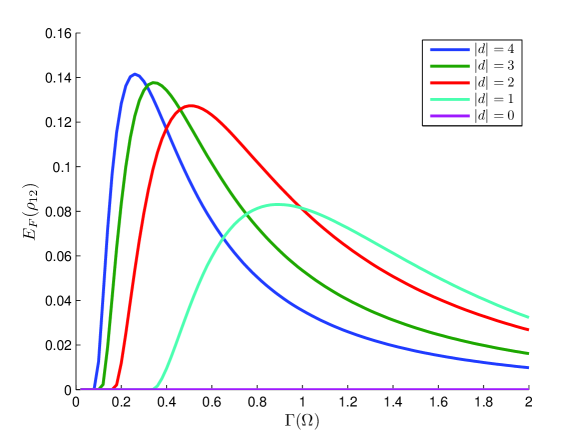
Figure 3: Increasing behaviour of the steady-state entanglement for $|d|$ growing from $0$ to $4$. The system is separable when $d=0$ (isotropic Heisenberg model). When $d$ increases, and the term $XXYY$ dominates, the range of values of $\Gamma$ for which the steady state is separable shrinks, while the maximum achievable steady state entanglement grows.

4 Steady state entanglement under transverse decoherence (pure dephasing)

Apart from processes describing emission or absorption of quanta, qubit implementations can undergo energy conserving, purely dephasing processes, where only the coherences are affected and the populations remain unchanged. This is the situation encountered when the interaction term with the bath is mediated by an operator that commutes with the qubit Hamiltonian. Given the system Hamiltonian of one qubit $H=(\omega_{0}/2)\sigma_{z}$, a feasible qubit–bath interaction is $V=\sigma_{z}X$ where the force operator is $X=\sum_{k}C_{k}(a_{k}+a_{k}^{\dagger})$. This leads, under the customary approximations, to the master equation

$$\frac{d\rho}{dt}=-i[H,\rho]+2\gamma(\sigma_{z}\rho\sigma_{z}-\rho),$$ (10)

where

$$\gamma=\frac{1}{2}\lim_{\omega\rightarrow 0}S_{X}(\omega)=\pi\lim_{\omega\rightarrow 0}\mathcal{J}(\omega)\coth\left(\frac{\omega}{2k_{\mathrm{B}}T}\right)$$

for a thermal bath with spectral density $\mathcal{J}(\omega)=\sum_{k}C_{k}^{2}\delta(\omega-\omega_{k})$.

This process can be embedded in our framework provided that the Rabi frequencies of the external driving $\Omega_{j}$ and the interqubit coupling $J$ are small enough in comparison with the free evolution frequencies HP07 . The master equation in the rotating picture for $N$ qubits is then given by

$$\frac{d\rho}{dt}=-i[H_{\mathrm{coh}},\rho]+2\sum_{j=1}^{N}\gamma_{j}(\sigma_{z}^{j}\rho\sigma_{z}^{j}-\rho).$$ (11)

In this situation the system no longer exhibits quantum correlations in the steady state. Indeed, the steady state of equation (11) is unique and it is the completely mixed state $\rho^{\mathrm{ss}}=\mathds{1}/N$. This result follows from theorem 5.2 in Sp80-Fr78 which asserts that given a steady state $\rho^{\mathrm{ss}}$ of a master equation written in the standard form

$$\frac{d\rho}{dt}=-i[H,\rho]+\sum_{j}\left(V_{j}\rho V_{j}^{\dagger}-\frac{1}{2}V_{j}^{\dagger}V_{j}\rho-\frac{1}{2}\rho V_{j}^{\dagger}V_{j}\right),$$

such that $\mathrm{rank}(\rho^{\mathrm{ss}})=N$, the given steady state is unique if the only operators commuting with $H$ and every $V_{j}$ are multiples of the identity. This is true for our case since the only operators that commute with both $\sigma_{x}$ and $\sigma_{z}$ (and therefore with $\sigma_{y}$ as well because of the Jacobi identity) are proportional to the identity because of Schur’s lemma.

5 SR phenomena under both longitudinal and transverse decoherence

The situation changes if we have both emission/absorption and pure dephasing processes in our system, as is the case in many solid state qubit implementations (see for example schoen and references therein). Then the master equation is modified according to

$$\frac{d\rho}{dt}=-i\left(H_{\mathrm{eff}}\rho-\rho H_{\mathrm{eff}}^{\dagger}\right)+\sum_{j}2\Gamma_{j}(\bar{n}+1)\sigma_{-}^{j}\rho\sigma_{+}^{j}+\sum_{j}2\Gamma_{j}\bar{n}\sigma_{+}^{j}\rho\sigma_{-}^{j}+\sum_{j}2\gamma_{j}\sigma_{z}^{j}\rho\sigma_{z}^{j},$$ (12)

where $\gamma_{j}$ denotes the pure dephasing rates, and $H_{\mathrm{eff}}$ is given by the same equation (3) with an additional term of the form $-i\sum_{j}\gamma_{j}$ accounting for pure dephasing.

Consider $T=0$ (also assuming that each $\gamma_{j}$ is finite). For two qubits in the absence of pure dephasing, the threshold for an entangled steady state was given in (6) to be HP07

$$\rho_{12}^{\mathrm{ss}}\ \mathrm{entangled}\Leftrightarrow\frac{1}{2s}<r.$$

We now want to do the same analysis with the pure dephasing term added. For simplicity let us assume $\gamma=\Gamma$. The result is now more complicated as shown in figure 4 where $J$ is plotted against $\Gamma$ ($s$ vs. $r$) without pure dephasing (red dashed line), and with pure dephasing (blue solid line dividing entangled and separable zones). For illustrative purposes we have included values of $J$ substantially larger than $\Omega$, whilst still adhering to the weak-coupling assumptions of the master equation.

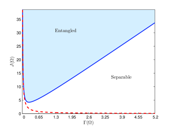
Figure 4: Steady state entangling behaviour: $J$ vs. $\Gamma$ without pure dephasing (red dashed line), and with pure dephasing (blue solid line). The blue shading shows the entangled zone in the presence of pure dephasing.

There are several differences between the two cases. For both cases, the steady state is separable for very small $\Gamma$, so it is necessary to include some appreciable amount of noise to produce entanglement (SR–like behaviour). However, in the presence of pure dephasing, only a finite amount of additional noise is required to come back to the separable regime. (Recall that an infinite amount of noise is required in the absence of pure dephasing.) Furthermore, in the presence of pure dephasing the SR–like behaviour disappears completely for small $J$, where the steady state remains separable. At odds with the monotonic result (6) of HP07 (red dashed line of figure 4), the nonmonotonicity of the blue solid threshold in figure 4 (note the minimum point) reflects in some sense the competition between both processes. Consider the simplest case where qubits were subject to a $ZZ$ coupling. In figure 5, where we plot the behaviour of the probabilities $P_{z}$ (localization) and $P_{x}$ (delocalization) for each qubit to be in an eigenstate of the corresponding Pauli operator (i.e., $\sigma_{z}$ or $\sigma_{x}$). The closer the local states are to an eigenstate of $\sigma_{z}$, the less effective the coherent $ZZ$ coupling is and the global state tends to be separable. The localization probability increases steadily with the transverse decay rate; however, the delocalization probability is maximal for some optimal noise strength provided that pure dephasing is not too large. The region around the maximum delocalization probability coincides with the maximum steady state entanglement.

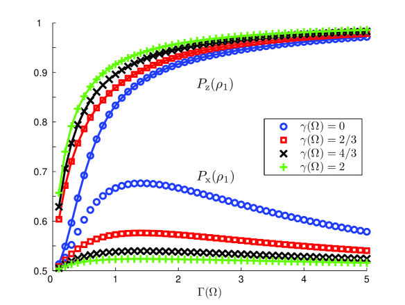
Figure 5: Illustration of the combined action of transverse and longitudinal decoherence on an array of $N=2$ qubits with a $ZZ$ interqubit Hamiltonian. Increasing the pure dephasing rate keeps the delocalization probability of single qubits $P_{\mathrm{x}}$ close to $1/2$ so that the qubits are in a state close to an eigenstate of their local Hamiltonians ($\sigma_{z}$) which reduces the entangling power of the coherent $ZZ$ coupling.

The exact form of the threshold is complicated note . An approximate solution for it is $s\simeq\frac{1}{2r}+\frac{32r+2}{5}$. So that the steady state is entangled for a noise strength in, approximately, the range

$$-1/32+(5/64)s-(1/64)\sqrt{25s^{2}-20s-316}<r<-1/32+(5/64)s+(1/64)\sqrt{25s^{2}-20s-316}$$

Note that the lower bound is always higher than the previous one, $1/2s$.

For the case of arbitrary values of $\gamma$ and $\Gamma$, the steady-state correlations are diminished as $\gamma$ increases. This can be visualized in the behaviour of bipartite entanglement, as illustrated in figure 6. In order to construct a proper information theoretic measure of SR, we consider the quantum mutual information $I_{M}$, defined for a general bipartite system AB as $I_{M}(\rho_{AB})=S(\rho_{A})+S(\rho_{B})-S(\rho_{AB})$, where the states $\rho_{A,B}$ are the local states $\rho_{A,B}=\mathrm{Tr}_{B,A}(\rho_{AB})$. This function quantifies the total correlation content in any bipartite system Henderson and is depicted in figure 7 for the case of a chain of 6 qubits. There we evaluate the mutual information of the first two qubits in the chain but should stress that the same qualitative behaviour, where total correlations are maximized for some optimal, intermediate value of the decay rate, are obtained when evaluating the quantum mutual information across any other bipartition in the chain. We note that having a nonzero detuning $\delta\neq 0$ does not change the shape of the entanglement function, but its magnitude is reduced; the effect being small for small detuning, say $\delta^{j}\sim 10^{-3}-10^{-2}$.

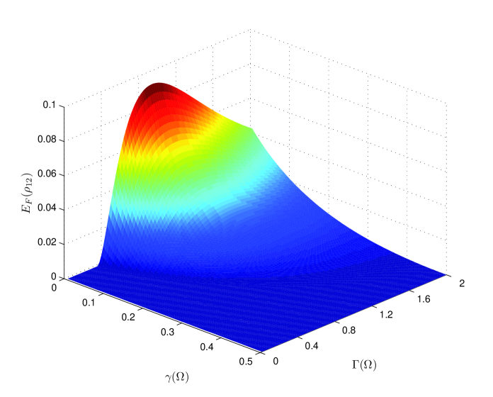
Figure 6: Quantum correlations in a two-qubit array as quantified by the entanglement of formation as a function of the noise parameters $\Gamma$ and $\gamma$ for $J/\Omega=1.5$. Note the monotonous negative effect when $\gamma$ increases so that as the pure dephasing rate increases, the larger it becomes the threshold value for the transverse decoherence until reaching a critical value $\gamma_{c}$ for which no entanglement survives in the steady state.

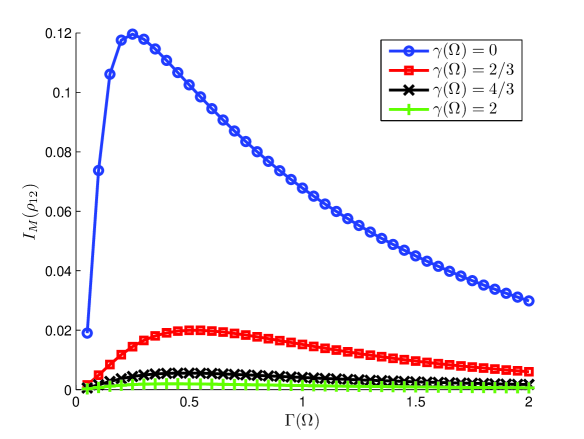
Figure 7: Quantum mutual information $I_{M}(\rho_{12})$ between qubits 1 and 2 in an $N=6$ array for different values of the dephasing rate $\gamma$ and variable transverse decoherence rate $\Gamma$ for $J/\Omega=1.5$. The same qualitative behaviour is observed for other pairs of neighbouring qubits or across different bipartitions within the system. The quantum mutual information is maximized for an optimal decay rate $\Gamma$ above which the total correlations in the system start to degrade. The larger the dephasing rate acting locally on the qubit systems, the smaller the value of the maximum correlation content becomes.

6 Conclusion

We have discussed the emergence of SR–like effects in composite spin systems subject to both decay (longitudinal decoherence) and pure dephasing (transverse decoherence). We have shown that quantum correlations vanish in the steady state if the local noise is purely transverse. Under pure dephasing, the system evolves into a maximally mixed state. When transverse and longitudinal noise are simultaneously present, for fixed dephasing, one encounters a decay rate threshold for steady–state entanglement to exist, provided that dephasing noise remains moderate. In the special case where $\Gamma=\gamma$, an approximate analytical threshold condition can be derived.

To quantitatively characterize the presence of stochastic resonance, we compute the total correlation content of the system, as quantified by its mutual information for bipartitions of arbitrary size, and show that it is a non-monotonic function of the decay rate $\Gamma$ (for fixed $\gamma$). We therefore argue that the system displays SR as measured by an information–theoretic figure of merit.

In the present work we have focussed our interest on the correlations content and, in particular, on the entanglement content of the steady state. These results show that a noisy environment does not just monotonically degrade the amount of entanglement but can act, for a suitable noise level, as a purifying mechanism that prevents the system from thermalizing — unless the noise becomes too strong plenio02 .

It seems to become more and more clear that the presence of environmental noise, far from being always detrimental, may actually be instrumental in the optimization of certain processes. So far this is more clear–cut in the case of processing classical information, as in the original SR concept of amplifying a weak signal, or the quantum setting in the context of the assisting transport of excitons across spin networks. Those can model for instance natural phenomena such as exciton transport in light–harvesting complexes aspuru ; bio ; olaya ; fleming . However, there are already indications that noise may also assist the transfer of quantum information, as exemplified by the enhanced fidelity in the transmission of quantum states demonstrated in difranco . It would be extremely important to generalize this result and to clearly identify the conditions under which not only quantum correlations, but also the transfer of quantum information, can be effectively assisted by noise.