Kinetic models for polymers with inertial effects

Abstract.

Novel kinetic models for both Dumbbell-like and rigid-rod like polymers are derived, based on the probability distribution function $f(t,x,n,\dot{n})$ for a polymer molecule positioned at $x$ to be oriented along direction $n$ while embedded in a $\dot{n}$ environment created by inertial effects. It is shown that the probability distribution function of the extended model, when converging, will lead to well accepted kinetic models when inertial effects are ignored such as the Doi models for rod like polymers, and the Finitely Extensible Non-linear Elastic (FENE) models for Dumbbell like polymers.

1. Introduction

In this paper we derive novel kinetic models for both Dumbbell like and rigid-rod like polymers in the presence of inertial forces. The model is to describe dynamics of the probability distribution function embedded in high dimensional configuration space due to inertial effects. We then prove that the limit equation of the new model when inertial force vanishes leads to current models with no inertial effects such as the FENE model and the Doi model, respectively. This illustrates consistency of our kinetic models with existing models.

The wide range of applications of polymer materials has attracted new areas of academic and industrial research. The synthesis of different type of polymers has enlarged the range of applications of polymer materials to areas where mechanical properties are important. Materials made up of macro-molecules such as polymers display properties that completely differ from those made from small molecules. The description of polymer dynamics is often based on large assemblies of molecules, the characteristics could be modeled in terms of their statistical properties.

Most polymers are long chains or branches of repeated chemical units. The full description of each atom in the polymer by molecular dynamics is not feasible for the huge computational effort. Coarse grained models are often expected with macroscopic space and time properties of complex fluids. Typical models such as bead-spring chain for flexible polymers and the rigid rod model for liquid crystalline polymers have been established by the pioneers in polymer science.

In general, the flow modeling of polymers has to take into account the internal structure, characterized by both positional and orientational order of phases. Such incorporation is often done by adding new balance equations to those that govern structure-less Newtonian fluids. These new balances must be evaluated from the behavior of polymers. According to the relative size of the bending persistence size and the length of the polymer, two canonical types of polymers are widely studied: the Dumbbell model and the rigid-rod like model. In modeling motion of polymers, it is essential to explore an accurate method of solutions of the Langevin equation for particles undergoing Brownian movement (rotational or translational) under the influence of external fields. A large number of reviews, text books and monographs on the theory, applications and rheology of polymeric materials have appeared in the literature, see e.g. [18, 19, 20, 17, 10, 11, 36, 8, 33, 24, 38].

There are three main levels of description of polymeric fluids: atomistic modeling, kinetic modeling [11, 20], and the macroscopic approach of continuum mechanics [36]. We shall exploit the kinetic approach. Models of kinetic theory provide a coarse-grained description of molecular configurations wherein atomistic processes are ignored altogether (Doi and Edwards [11], Bird et al [36], and Ottinger[33]). Kinetic theory models for polymer solutions are most naturally exploited numerically by means of stochastic simulation or Brownian dynamics methods [33]. A kinetic theory model when equipped with an expression relating stress to molecular configurations plays an important role in developing micro-macro methods of computational rheology [35, 23]. In current kinetic theory models for polymers, the inertia of molecules is often neglected. However, neglect of inertia in some cases leads to incorrect predictions of the behavior of polymers. The forgoing considerations indicate that the inertial effects are of importance in practical applications, e.g., for short time characteristics of materials based on the relevant underlying phenomena.

It is thus the goal of this paper to model dynamics of the density distribution of polymers when the inertial force is no longer ignorable. More precisely we shall be particularly interested in modeling two canonical types of polymers: Dumbbell-like and rod-like polymers, which when inertial forces are not considered have been well understood. We first derive kinetic models including inertial effects from particle dynamics (continuum limit in the Brownian motion), we then show the limit of the augmented models when inertial forces vanish leads to the inertia-free model.

We now summarize our main results for two types of polymers.

1.1. Dumbbell-like polymers

A mcromolecule is idealized as an ‘elastic dumbbell’ consisting of two ‘beads’ joined by a spring which can be modeled by an end-to-end vector $n$. Here $n$ is in a bounded ball $B(0,n_{0})$, which means that the extensibility of the polymers is finite. Let $f(t,x,n,p,q)$ denote the distribution function of Dumbbell-like polymers on the space variables $x\in\mathbb{R}^{d}$, $d=2,3$, the translational velocity $p\in\mathbb{R}^{d}$, the end-to-end vector $n$ as well as the orientational velocity $q\in\mathbb{R}^{d}$. And $t$ is the time. The novel kinetic model to be derived is

$$\partial_{t}f+\nabla_{x}\cdot(pf) +\nabla_{n}\cdot(qf)+\nabla_{p}\cdot(-\frac{\zeta}{m}(p-u(x))f)$$ (1.1)

$$+\nabla_{q}\cdot\left(\left(-\frac{\zeta}{m}(q-n\cdot\nabla_{x}u(x))-\frac{2F}{m}\right)f\right)=\frac{2k_{B}T\zeta}{m^{2}}[\Delta_{p}f+\Delta_{q}f],$$

where $\zeta$ is the frictional coefficient for the beads with mass $m$, $k_{B}$ is the usual Boltzmann constant, $T$ is the absolute temperature, and $F$ is the spring force between beads. The force usually derives from a potential, and has different forms for different models. For the well known FENE potential

$$F=\frac{Hn}{1-n^{2}/n^{2}_{0}},$$

where $H$ is a spring constant [36].

The above model under the scaling

$$m=\epsilon^{2},\quad\sqrt{m}p\to p,\quad\sqrt{m}q\to q,$$

leads to

$$\epsilon^{2}\partial_{t}f +\epsilon\nabla_{x}\cdot(pf)+\epsilon\nabla_{n}\cdot(qf)$$

$$+\epsilon\nabla_{p}\cdot(\zeta u(x)f)+\epsilon\nabla_{q}\cdot[(\zeta n\cdot\nabla_{x}u-2F)f]=Q(f),$$ (1.2)

where

$$Q(f):=\zeta\nabla_{p}\cdot(pf+2k_{B}T\nabla_{p}f)+\zeta\nabla_{q}\cdot(qf+2k_{B}T\nabla_{q}f).$$

Our result for Dumbbell like polymers could thus read as follows:

Theorem 1.1.

The limit $\epsilon\to 0$ of $f$ is given by $f^{0}=\rho M$ where $\rho=\rho(t,x,n)\geq 0$ and $M$ are given by

$$\rho(t,x,n)=\int f^{0}(t,x,n,p,q)dpdq,\quad M=\exp\left(-\frac{p^{2}+q^{2}}{4k_{B}T}\right).$$

Furthermore, $\rho(t,x,n)$ satisfies the following kinetic equation

$$\partial_{t}\rho+\nabla_{x}\cdot(u(x)\rho)+\nabla_{n}\cdot((n\cdot\nabla_{x}u-\frac{2F}{\zeta})\rho)=\frac{2k_{B}T}{\zeta}\Delta_{x}\rho+\frac{2k_{B}T}{\zeta}\Delta_{n}\rho.$$ (1.3)

1.2. Rod-like polymers

Polymers are idealized as rods of fixed length. The orientation space is $n\in\mathbb{S}^{d-1}$. Let $f(t,x,n,p,\omega)$ denote the distribution function of rod-like polymers on the space variables $x\in\mathbb{R}^{d}$, the translational velocity $p\in\mathbb{R}^{d}$, the orientational vector $n$ as well as the angular velocity $\omega$. Here $\omega$ is on the tangent bundle $T_{n}\mathbb{S}^{d-1}$. And $t$ is the time. Our rescaled kinetic model can be formulated as

$$\epsilon\partial_{t}f +\nabla_{x}\cdot(pf)+\mathcal{R}\cdot(\omega f)+\zeta_{t}\nabla_{p}\cdot(u(x)f)$$

$$+\nabla_{\omega}\cdot((\zeta_{r}n\times\nabla_{x}u\cdot n-\mathcal{R}\cdot U)f)=\frac{1}{\epsilon}Q(f),$$ (1.4)

where

$$Q(f)=\zeta_{t}\nabla_{p}\cdot(pf+k_{B}T\nabla_{p}f)+\zeta_{r}\nabla_{\omega}\cdot(f\omega+k_{B}T\nabla_{\omega}f).$$

Here $\epsilon$ denotes the inertial parameter similar to (1.1), $u$ is the fluid velocity, and $U$ is certain interaction potential of rods. $\mathcal{R}=n\times\nabla_{n}$ is the rotational gradient operator, and $k_{B},T$ denote the Boltzmann constant and absolute temperature, respectively. $\zeta_{t},\zeta_{r}$ are frictional coefficients in $x$ and $n$ directions.

Our result for rod-like polymers then reads as follows:

Theorem 1.2.

The formal limit $\epsilon\to 0$ of $f$ is given by $f^{0}=\rho M$ where $\rho=\rho(t,x,n)\geq 0$ and $M$ are given by

$$\rho(t,x,n)=\int f^{0}(t,x,n,p,q)dpd_{n}\omega,\quad M=\exp\left(-\frac{p^{2}+\omega^{2}}{2k_{B}T}\right).$$

Furthermore, $\rho(t,x,n)$ satisfies the kinetic equation

$$\partial_{t}\rho+\nabla_{x}\cdot(u(x)\rho)+\mathcal{R}\cdot(n\times\nabla_{x}u\cdot\rho)=D_{t}\Delta_{x}\rho+D_{r}\mathcal{R}\cdot\left[\mathcal{R}\rho+\frac{\rho}{k_{B}T}\mathcal{R}U\right]$$ (1.5)

where

$$D_{t}=\frac{k_{B}T}{\zeta_{t}},\quad D_{r}=\frac{k_{B}T}{\zeta_{r}}.$$

Our derivation of these kinetic models is based on establishing motion laws of polymer molecules, followed by a conversion into the kinetic description. The formal limit when inertia vanishes is justified by taking the classical approach for hydrodynamic limits. To this end a rescalling is adopted, so that the collision operator is set on fast scale, and the dissipation of the collision operator drives the states to the unique equilibrium states $M$. Derivation of models for Dumbbell-like polymers and the formal limit justification are given in §3, and those for rod-like polymers are given in §4. Some concluding remarks are presented in §5.

Finally, we wish to close this section by pointing to a vast body of recent work on mathematical treatment of kinetic theory models for polymers, their constitutive models as well as their coupling with fluid models (so called micro-macro models), see e.g. [37, 9, 14, 4, 3, 13, 22, 1, 6, 7, 16, 12, 31, 15, 21, 39, 2, 30, 26, 28, 5, 25, 29, 27, 32, 34, 41, 40] and references therein. These should provide guidance in establishing the various levels of mathematical theory of kinetic models developed in this work.

2. Kinetic models for Dumbbell polymers

2.1. Equations of motion with non-trivial inertia

We consider a polymer consisting of two-beads connected by one-spring. Each bead as a coarse grained particle represents several chemical units and experiences four kinds of forces in the dilute case where there is no interaction for inter–and intra-dumbbells.

Assume the two beads are positioned at $x_{1}$ and $x_{2}$, the Langevin equation of the beads are just balance of different forces expressed as

$$m_{1}\ddot{x_{1}} =-\zeta_{1}(\dot{x}_{1}-u(x_{1}))+F_{1}+\sigma_{1}\dot{W}_{1},$$

$$m_{2}\ddot{x_{2}} =-\zeta_{2}(\dot{x}_{2}-u(x_{2}))+F_{2}+\sigma_{2}\dot{W}_{2}.$$

Here $W_{i}$ are independent standard Brownian motions, $\zeta_{i}$ are frictional coefficients for the $i$-th bead with mass $m_{i}$, $\sigma_{i}=\sqrt{2k_{B}T\zeta_{i}}$ by fluctuation-dissipation theorem, where $k_{B}$ is the Boltzmann constant, and $T$ is the temperature. The spring forces $F_{1}=-F_{2}=F$ by Newton’s Third Law depends only on the end-to-end vector $n$.

A natural configuration for this underlying polymer includes both position of the polymer with these two beads connected to one spring

$$x=\frac{x_{1}+x_{2}}{2},$$

and the end-to-end vector denoted by $n=x_{2}-x_{1}$. We assume that $m_{1}=m_{2}=m$ and $\zeta_{1}=\zeta_{2}=\zeta$. Then the difference and average of the above two equations gives a coupled system

$$m\ddot{x} =-\zeta(\dot{x}-u(x))+\sqrt{4k_{B}T\zeta}\dot{W}_{1},$$ (2.1)

$$m\ddot{n} =-\zeta(\dot{n}-n\cdot\nabla_{x}u)-2F+\sqrt{4k_{B}T\zeta}\dot{W}_{2}.$$ (2.2)

The approximation utilizes the equation $u(x)\sim(u(x_{1})+u(x_{2}))/2$, $u(x_{2})-u(x_{1})\sim\nabla_{x}u\cdot n$, and the two new Brownian motions $(W_{2}\pm W_{1})/\sqrt{2}$ (still denoted by $W_{i}$).

If the inertia were ignored for this two beads spring system, we would have the following stochastic equations (SDE),

$$\dot{x} = u(x)+\sqrt{\frac{4k_{B}T}{\zeta}}\dot{W}_{1},$$ (2.3)

$$\dot{n} = n\cdot\nabla_{x}u-\frac{2F}{\zeta}+\sqrt{\frac{4k_{B}T}{\zeta}}\dot{W}_{2}.$$ (2.4)

The differential operator or the infinitesimal generator corresponding to the process $(x(t),n(t))$ is given by

$$L\equiv\langle u(x),\nabla_{x}\rangle+\langle n\cdot\nabla_{x}u-\frac{2F}{\zeta},\nabla_{n}\rangle+\frac{2k_{B}T}{\zeta}(\Delta_{x}+\Delta_{n}),$$ (2.5)

where

$$\nabla_{x}=\left(\frac{\partial}{\partial_{x_{1}}},\cdots,\frac{\partial}{\partial_{x_{d}}}\right),\quad\nabla_{n}=\left(\frac{\partial}{\partial_{n_{1}}},\cdots,\frac{\partial}{\partial_{n_{d}}}\right),$$

with $\langle,\rangle$ denoting the Euclidean inner product in $\mathbb{R}^{d}$. The configuration of Dumbbell like polymers can be illustrated in Figure 1:

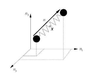
Figure 1. A Dumbbell like polymer

When inertial force is significant, one has to take the inertial effects into consideration. We now rewrite the system (2.1)-(2.2) into a first-order system

$$\dot{x} =p,$$

$$\dot{n} =q,$$

$$\dot{p} =-\frac{\zeta}{m}(p-u(x))+\frac{\sqrt{4k_{B}T\zeta}}{m}\dot{W}_{1},$$

$$\dot{q} =-\frac{\zeta}{m}(q-n\cdot\nabla_{x}u(x))-\frac{2F}{m}+\frac{\sqrt{4k_{B}T\zeta}}{m}\dot{W}_{2}.$$

This system can be considered as a degenerate stochastic differential equation with a singular diffusion matrix of $4d\times 4d$. The differential operator corresponding to the process $(x(t),n(t),p(t),q(t))$ is also uniquely defined. In fact for the above dissipative stochastic differential equation with well-defined initial data, a unique solution $(x,n,p,q)(t)$ up to an explosion time is ensured if $u(x)$ and $F$ are smooth functions of the configuration variables.

2.2. Kinetic description

We now formulate the kinetic description of the above motion laws. For a given instant $t$, the random variables $X=(x,n,p,q)$ can be characterized by a probability density function (PDF) $f(t,x,n;p,q)$ defined by

$$f(t,x,n;p,q,)dX=P[\{X\leq\tilde{X}\leq X+dX\}].$$

In words, the right-hand side is the probability that the random variable $\tilde{X}$ falls between the sample space values $X$ and $X+dX$ for different realizations of the polymer motion. Thus the above statistical ODE system can be converted into a PDE of the form

$$\partial_{t}f+\nabla_{x}\cdot(pf) +\nabla_{n}\cdot(qf)+\nabla_{p}\cdot\left(-\frac{\zeta}{m}(p-u(x))f\right)$$ (2.6)

$$+\nabla_{q}\cdot\left(\left(-\frac{\zeta}{m}(q-n\cdot\nabla_{x}u(x))-\frac{2F}{m}\right)f\right)=\frac{2k_{B}T\zeta}{m^{2}}[\Delta_{p}f+\Delta_{q}f].$$

It is known that in the case with no inertial forces the kinetic equation is also of the Fokker-Planck type. The model follows from the motion law (2.3)-(2.4) as follows:

$$\partial_{t}\rho+\nabla_{x}\cdot(u(x)\rho)+\nabla_{n}\cdot\left(\left(n\cdot\nabla_{x}u-\frac{2F}{\zeta}\right)\rho\right)=\frac{2k_{B}T}{\zeta}\Delta_{x}\rho+\frac{2k_{B}T}{\zeta}\Delta_{n}\rho,$$ (2.7)

where $\rho(t,x,n)$ denotes the corresponding probability density function.

Remark 2.1.

The polymer scale is much smaller than the fluid scale, the diffusion in space is often ignorable. Here we make no such distinction.

It is natural to ask whether the effective dynamics in (2.6) is dominated by (2.7) when inertia vanishes. As a first step we shall identify an effective equation satisfied by the limit of $f$ when $m\downarrow 0$, if the limit exists. In the remainder, we will always suppose that $f$ is as smooth as needed.

2.3. Scaling

We make the following scaling

$$m=\epsilon^{2},\quad\sqrt{m}p\to p,\quad\sqrt{m}q\to q,$$

to obtain

$$\epsilon^{2}\partial_{t}f+\epsilon\nabla_{x}\cdot(pf)+\epsilon\nabla_{n}\cdot(qf)+\epsilon\nabla_{p}\cdot(\zeta u(x)f)+\epsilon\nabla_{q}\cdot[(\zeta n\cdot\nabla_{x}u-2F)f]=Q(f),$$ (2.8)

where

$$Q(f):=\zeta\nabla_{p}\cdot(pf+2k_{B}T\nabla_{p}f)+\zeta\nabla_{q}\cdot(qf+2k_{B}T\nabla_{q}f).$$

The remaining task in this section is to justify the following

Theorem 2.1.

The limit $\epsilon\downarrow 0$ of the $f^{\epsilon}$ is given by $f^{0}=\rho(t,x,n)M(p,q)$, where

$$M=\exp\left(-\frac{p^{2}+q^{2}}{4k_{B}T}\right)$$ (2.9)

satisfying $Q(M)=0$ and $\rho(t,x,n)$ solves the kinetic equation (2.7).

As usual the limit equation that is associated with (2.8) does not depend on details of the operator $Q$. Rather, it depends on $Q$ possessing certain properties related to conservation, dissipation, and equilibria that are stated below. Note the operator $Q$ acts on the augmented variables $(p,q)$ only and leaves other variables $(t,x,n)$ as parameters. Thus we list some properties of $Q$ as an operator acting on functions of $(p,q)$ only, which are essential in the derivation of the limit equation.

2.4. Properties of $Q$

Note that the operator $Q(f)$ has the following properties

• The operator can be written as a conservative form

  $$Q(f)=2\zeta k_{B}T\nabla_{p,q}\cdot\left(M\nabla_{p,q}\left(\frac{f}{M}\right)\right).$$

• The conservation form leads to

  $$\int Q(f)dpdq=0$$

  for every $f\in L^{1}(dpdq)$. This relation expresses the physical laws of mass conservation during the action of $Q$.

  Moreover, this is the only such conservation law. This means that

  $$\int Q(f)\psi dpdq=0,\quad\forall f\Leftrightarrow\psi\in{\rm span}\{1\}.$$

• Dissipation. There is a nonnegative function $\eta(f)$ that is an entropy for the operator $Q$. This means that for $\eta(f)\in L^{1}(dpdq)$ we have

  $$\int\eta^{\prime}(f)Q(f)\leq 0,$$

  whose vanishing characterizes the local equilibrium of $Q$. For flexible polymers, $\eta^{\prime}(f)=f/M$ since

  $$D^{Q}(f)=\int Q(f)\frac{f}{M}dpdq=-\int M\left(\nabla_{p,q}\left(\frac{f}{M}\right)\right)^{2}dpdq\leq 0.$$

• Existence of equilibria. From the above dissipation property we see that the function $f(p,q)$ such that $Q(f)=0$ forms a space identified through

  $$\frac{f}{M}\in{\rm span}\{1\}.$$

  This equilibrium is unique up-to a constant multiplier. We normalize the density function then

  $$f_{eq}=\left[\int Mdpdq\right]^{-1}M.$$

2.5. Asymptotic limit as $\epsilon\downarrow 0$

Equipped with these properties we now investigate the asymptotic limit. Define

$$\rho^{\epsilon}(t,x) =\int fdpdq,$$

$$J_{1}^{\epsilon}(t,x) =\frac{1}{\epsilon}\int pfdpdq,$$

$$J_{2}^{\epsilon}(t,x) =\frac{1}{\epsilon}\int qfdpdq.$$

Then integration of (2.8) together with conservation property of $Q$ yields

$$\partial_{t}\rho^{\epsilon}+\nabla_{x}\cdot J_{1}+\nabla_{n}\cdot J_{2}=0,\quad\forall\epsilon>0.$$ (2.10)

We suppose that as $\epsilon\downarrow 0$ the limit of $f$ is identified by $f^{0}$. It follows from the equation (2.8) that

$$f^{0}\in Q^{-1}(0).$$

This implies that $f^{0}=M(p,q)\rho^{0}(t,x,n)$, for the operator $Q$ does not act on $(t,x,n)$. Hence the probability density function $f$ takes the following form

$$f^{\epsilon}(t,x,n;p,q)=\rho^{\epsilon}(t,x,n)M(p,q)+\epsilon g^{\epsilon},$$

where

$$\lim_{\epsilon\downarrow 0}\rho^{\epsilon}(t,x,n)=\rho^{0}(t,x,n).$$

Note that $\int pMdpdq=\int qMdpdq=0$, we thus have

$$J_{1}^{\epsilon} =\frac{1}{\epsilon}\int pf^{\epsilon}dpdq=\int pg^{\epsilon}dpdq,$$ (2.11)

$$J_{2}^{\epsilon} =\frac{1}{\epsilon}\int qf^{\epsilon}dpdq=\int qg^{\epsilon}dpdq.$$ (2.12)

The limit of these flux functions depends only on the limit of $g^{\epsilon}$.

Linearity of the operator $Q$ and $Q(M)=0$ leads to

$$Q(f^{\epsilon})=Q(\rho^{\epsilon}(t,x)M(p,q)+\epsilon g^{\epsilon})=\epsilon Q(g^{\epsilon}).$$

Using the equation (2.8) we obtain

$$Q(g^{\epsilon}) =\frac{1}{\epsilon}Q(f^{\epsilon})$$

$$=\epsilon\partial_{t}f^{\epsilon}+\nabla_{x}\cdot(pf^{\epsilon})+\nabla_{n}\cdot(qf^{\epsilon})+\nabla_{p}\cdot(\zeta u(x)f^{\epsilon})+\nabla_{q}\cdot((\zeta n\cdot\nabla_{x}u-2F)f^{\epsilon})$$

$$=\nabla_{x}\cdot(pM\rho^{\epsilon})+\nabla_{n}\cdot(qM\rho^{\epsilon})+\nabla_{p}\cdot(\zeta u(x)\rho^{\epsilon}M)$$

$$\qquad+\nabla_{q}\cdot((\zeta n\cdot\nabla_{x}u-2F)M\rho^{\epsilon})+O(\epsilon).$$

Let $g^{\epsilon}\to g^{0}$ as $\epsilon\to 0$, then it is clear that

$$Q(g^{0})=p\cdot\nabla_{x}\rho^{0}M+q\cdot\nabla_{n}\rho^{0}M+\zeta\rho^{0}u(x)\cdot\nabla_{p}M+\rho^{0}(\zeta n\cdot\nabla_{x}u-2F)\cdot\nabla_{q}M.$$

Again note that $Q$ is a linear operator, we may assume the ansatz for $g^{0}$ as follows.

$$g^{0}=a\cdot\nabla_{x}\rho^{0}+b\cdot\nabla_{n}\rho^{0}+\zeta\rho^{0}c\cdot u(x)+\rho^{0}(\zeta n\cdot\nabla_{x}u-2F)\cdot d.$$

In comparison with the expression of $Q(g^{0})$ above, we see that it is sufficient to find $a,b,c,d$ such as

$$Q(a) =pM,$$

$$Q(b) =qM,$$

$$Q(c) =\nabla_{p}M,$$

$$Q(d) =\nabla_{q}M.$$

These relations are understood in the sense that the operator acts on each component of the underlying vector. In order to identity $(a,b,c,d)$ we state the following lemma:

Lemma 2.1.

Let $Q$ be the collision operator and $g\in L^{2}(R^{p}\times R^{q})$ such that $\int gdpdq=0$. The problem

$$Q(\psi)=g,$$ (2.13)

has a unique weak solution in $\Lambda=\{\psi,\quad\int\psi dpdq=0,\quad\psi\in H^{1}\}.$

This lemma, following from applying the Lax-Milgram theorem to the corresponding variational formulation, ensures that there exists unique $a,b,c,d$ in the space $\{\phi|\int\phi dpdq=0\}$ since

$$\int\{pM,qM,\nabla_{p}M,\nabla_{q}M\}dpdq=0.$$

We also note that from

$$\nabla_{p}M=-\frac{1}{2k_{B}T}pM,\quad\nabla_{q}M=-\frac{1}{2k_{B}T}qM,$$

it follows

$$c=-\frac{a}{2k_{B}T},\quad d=-\frac{b}{2k_{B}T}.$$

It remains to determine only $a$ and $b$. Let $a=\alpha Mp$ we have

$$Q(a)=-\alpha\zeta pM=pM,$$

which gives $\alpha=-\frac{1}{\zeta}$, leading to $a=-\frac{1}{\zeta}pM$. Similarly we obtain $b=-\frac{1}{\zeta}qM$.

Clearly we see that

$$\int\{b,d\}\cdot pdpdq=0,\quad\int\{a,c\}\cdot qdpdq=0.$$

These enable us to determine the asymptotic limits of the fluxes.

$$J_{1}^{0} =\int pg^{0}dpdq$$

$$=\int(a\cdot\nabla_{x}\rho^{0})p+\int(b\cdot\nabla_{n}\rho^{0})p+\zeta\rho^{0}\int(c\cdot u(x))p+\rho^{0}\int d\cdot(\zeta n\cdot\nabla_{x}u-2F)p$$

$$=\int a\cdot\left(\nabla_{x}\rho^{0}-\frac{\zeta u(x)\rho^{0}}{2k_{B}T}\right)pdpdq$$

$$=-\left(\nabla_{x}\rho^{0}-\frac{\zeta u(x)\rho^{0}}{2k_{B}T}\right)\frac{2k_{B}T}{\zeta}\int Mdpdq.$$

$$J_{2}^{0} =\int qg^{0}dpdq$$

$$=\int(a\cdot\nabla_{x}\rho^{0})q+\int b\cdot\nabla_{n}\rho^{0}q+\zeta\rho^{0}\int(c\cdot u(x))q+\rho^{0}\int d\cdot(\zeta n\cdot\nabla_{x}u-2F)q$$

$$=\int b\cdot\left(\nabla_{n}\rho^{0}-\frac{\rho^{0}}{k_{B}T}(\zeta n\cdot\nabla_{x}u-2F)\right)qdpdq$$

$$=-\left(\nabla_{n}\rho^{0}-\frac{\rho^{0}}{2k_{B}T}(\zeta n\cdot\nabla_{x}u-2F)\right)\frac{2k_{B}T}{\zeta}\int Mdpdq.$$

Now the equation (2.10) divided by $\int Mdpdq$ asymptotically converges to

$$\partial_{t}\rho^{0}+\nabla_{x}\cdot(u(x)\rho^{0})+\nabla_{n}\cdot((n\cdot\nabla_{x}u-\frac{2F}{\zeta})\rho^{0})=\frac{2k_{B}T}{\zeta}\Delta_{x}\rho^{0}+\frac{2k_{B}T}{\zeta}\Delta_{n}\rho^{0}.$$

This is exactly the equation (2.7) derived from ignoring inertial forces.

Remark 2.2.

With these kinetic equations for Dumbell like polymers, it is natural to understand how these polymers contribute to the macroscopic flow governed by a coupled Navier-Stokes system

$$\partial_{t}u+(u\cdot\nabla_{x}u)u+\nabla_{x}p=\frac{\gamma}{Re}\Delta_{x}u+\frac{1-\gamma}{ReDe}\nabla_{x}\cdot\tau,\quad\nabla_{x}\cdot u=0,$$

with the stress determined by

$$\tau=\int(n\otimes F)fdndpdq.$$

Here $De$ is called Deborah number, which is the most important parameter in non-Newtonian fluids. $Re$ and $\gamma$ are the Reynolds number and viscosity ratio, respectively. The tensor force follows the case when inertial force is ignored, the derivation of the tensor force with inclusion of inertial effects is beyond the scope of this work.

Remark 2.3.

The spring force is determined by a potential function $U$ through $F=-\nabla_{n}U$. Different potential leads to different models. Two choices are commonly used:

	Force	Potential
Hookean spring	$Hn$	$\frac{1}{2}Hn^{2}$
FENE spring	$\frac{Hn}{1-(n/n_{0})^{2}}$	$-\frac{1}{2}Hn_{0}^{2}ln\left(1-(n/n_{0})^{2}\right)$

where $n_{0}$ is the maximum extension of the beads connector.

3. Rigid rod-like polymers

Though many polymers are flexible, there is still a large class of polymers which are not flexible and assume a rod-like structure. Rod-like polymers have some peculiar properties and have attracted a great deal of attention.

We consider rod-like molecules in concentrated regime. Rod-like polymers can have only two kinds of motion, i.e., translation and rotation. The translational Brownian motion is the random motion of the position vector $x$ of the center of mass, and the rotational Brownian motion is the random motion of the unit vector $n$ ($|n|=1$) which is parallel to the polymer. We shall build a kinetic model for the probability distribution of orientational motions of rod in every point of phase space $(x,p)$. This serves as a microscopic equation, which is expected to be coupled with the macroscopic equation (the Navier-Stokes equation) for the fluid velocity.

For the convenience of calculations in what follows, we introduce a local coordinate on the sphere $\mathbb{S}^{2}$ as $q=(\theta,\phi)$, and set $n=(sin\theta cos\phi,sin\theta sin\phi,cos\theta)$ with $\theta\in[0,\pi)$ and $\phi\in[0,2\pi)$. The unit vector $e_{\theta}=(cos\theta cos\phi,cos\theta sin\phi,-sin\theta)$ and $e_{\phi}=(-sin\phi,cos\phi,0)$. We note that $\frac{\partial n}{\partial\theta}=e_{\theta}$, $\frac{\partial n}{\partial\phi}=sin\theta e_{\phi}$. Thus, any tangent vector on the sphere is written as

$$\dot{n}=\dot{\theta}e_{\theta}+\dot{\phi}sin\theta e_{\phi},$$

which gives

$$\omega=n\times\dot{n}=\dot{\theta}e_{\phi}-sin\theta\dot{\phi}e_{\theta}.$$

The gradient is

$$\nabla_{n}=e_{\theta}\partial_{\theta}+\frac{e_{\phi}}{sin\theta}\partial_{\phi}.$$

The rotational gradient is

$$\mathcal{R}=n\times\nabla_{n}=\left(-\frac{cos\phi cos\theta}{sin\theta}\partial_{\phi}-sin\phi\partial_{\theta},-\frac{cos\theta sin\phi}{sin\theta}\partial_{\phi}+cos\phi\partial_{\theta},\partial_{\phi}\right)^{T}.$$ (3.1)

Divergence of a vector $A=A_{\theta}e_{\theta}+A_{\phi}e_{\phi}$ is

$$\nabla_{n}\cdot A=\frac{1}{sin\theta}\partial_{\theta}(sin\theta A_{\theta})+\frac{1}{sin\theta}\partial_{\theta}A_{\phi}.$$

The gradient in terms of $\omega$ is defined only for a given $n$, and will be understood from now on as

$$n\cdot\nabla_{\omega}f=0,\quad\forall f.$$

To be more specific, we regard the identical liquid crystal molecules as inflexible rods of a thickness $b$ which is much smaller than their length $L$, as illustrated in Figure 2:

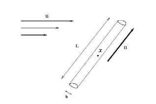
Figure 2. A rod like polymer

3.1. Translational Brownian motion

Let $U$ be an interaction potential, the force thus induced is $-\nabla_{x}U$. The motion law is

$$m\ddot{x}=-\zeta_{t}(\dot{x}-u(x))-\nabla_{x}U,$$

where $\zeta_{t}$ is the friction coefficient and $u(x)$ is the fluid velocity field. If $f$ is the probability distribution in $x$, the Brownian force is expressed as $F_{B}=-\nabla_{x}(k_{B}Tlnf)$, where $-k_{B}Tlnf$ is the chemical potential. For nontrivial inertial force, the distribution needs to be accounted in an extended environment with inclusion of $p=\dot{x}$. The corresponding translational Brownian force thus reduces to

$$F_{B}=\nabla_{p}W,\quad W=-\frac{\zeta_{t}k_{B}T}{m}lnf.$$ (3.2)

This can be justified by a similar derivation based on Brownian motions as that in Section 2. The scaled coefficient reflects balances between the friction force and the inertial force. Putting together we have the following translational motion law

$$\dot{x} =p,$$ (3.3)

$$\dot{p} =-\frac{\zeta_{t}}{m}(p-u(x))-\frac{1}{m}\nabla_{x}U-\frac{\zeta_{t}}{m^{2}}\nabla_{p}(k_{B}Tlnf).$$ (3.4)

In what follows we shall conveniently use the chemical potential to describe the Brownian force.

3.2. Rotational Brownian motion

We consider a rod rotating with angular velocity $\omega$, then the rotational motion can be described as

$$[J]\dot{\omega}=T,$$

where $J$ is the moment of inertia and $T$ is the total torque.

1. Rotational frictional force.

Consider a rod of length $L$ placed in a viscous fluid with fluid velocity $u(x)$, where $x$ is the center of mass of the rod.

The rod is parameterized by $s$, ranging from $-L/2$ to $L/2$, then the position vector of the $s$-point on this rod is written as

$$x(s)=x+ns,\quad x(0)=x,\quad-L/2\leq s\leq L/2.$$

Let $v(s)$ and $F(s)$ be the velocity of this point, and forces acting on it. The velocity $v(s)$ is expressed by the angular velocity $\omega$

$$v(s)=\omega\times(x(s)-x)=\omega\times(ns).$$

The frictional force at $x(s)$ is

$$F(s)=-\xi(s)(v(s)-u(x(s))),$$

where $\xi(s)$ is the frictional coefficient, being symmetric $\xi(s)=\xi(-s)$. Note that

$$u(x(s))\simeq u(x)+\nabla_{x}u(x(s)-x(0))=u(x)+s\nabla_{x}u\cdot n.$$

The frictional force thus reduces to

$$F(s)=-s\xi(s)(\omega\times n-\nabla_{x}u\cdot n)+\xi(s)u(x).$$

Thus the total torque induced by the frictional force acting on the rod is

$$T =\frac{1}{L}\int^{L/2}_{-L/2}(x(s)-x)\times F(s)ds$$

$$=-\xi_{2}n\times(\omega\times n-\nabla_{x}u\cdot n)+\xi_{1}n\times u(x),$$

where

$$\xi_{k}=\frac{1}{L}\int_{-L/2}^{L/2}s^{k}\xi(s)ds,\quad k=1,2.$$

Symmetry of $\xi(s)=\xi(-s)$ leads to $\xi_{1}=0$. Then using $n\cdot\omega=0$ we have

$$T=-\zeta_{r}\left[(Id-n\otimes n)\omega-n\times(\nabla_{x}u\cdot n)\right]=-\zeta_{r}\left[\omega-n\times(\nabla_{x}u\cdot n)\right],$$

where $\zeta_{r}=\xi_{2}$ denotes the rotational friction coefficient.

2. Thermodynamic potential force.

From $[J]\dot{\omega}=T$ it follows

$$\frac{d}{dt}E=T\cdot\omega,\quad E=\frac{1}{2}\omega^{\top}[J]\omega.$$

Let the potential be denoted by $U$. Then $d(E+U)=0$ gives $dE=-dU=-\nabla_{n}U\cdot dn.$

Note that from $|n|=1$ we have

$$\omega=n\times\dot{n},$$

which leads to

$$\omega dt=n\times dn.$$

We thus have

$$T\cdot(n\times dn)=T\cdot\omega dt=dE=-\nabla_{n}U\cdot dn.$$

Therefore $T\times n=-\nabla_{n}U$, i.e.,

$$T=-\mathcal{R}U,$$ (3.5)

where $\mathcal{R}$ is the rotational gradient operator given by (3.1).

3. Rotational Brownian force.
The following property will be used on our derivation of forces below.

Lemma 3.1.

For a fixed vector $a$, let $x=a\times y$. Then for any function smooth $g$,

$$\nabla_{y}g=-a\times\nabla_{x}g$$

and

$$a\cdot\nabla_{y}g=0,\quad\forall g.$$

Proof.

Let $\epsilon_{ijk}$ as the usual permutation symbol, then $x_{i}=\sum_{j,k}\epsilon_{ijk}a_{j}y_{k}$. We thus have

$$(\nabla_{y}g)_{m} =\sum_{i}\partial_{x_{i}}g\frac{\partial x_{i}}{\partial y_{m}}=\sum_{i}\partial_{x_{i}}g\sum_{j,k}\epsilon_{ijk}a_{j}\delta_{mk}$$

$$=\sum_{i,j}\epsilon_{mij}\partial_{x_{i}}ga_{j}=-\sum_{i,j}\epsilon_{mji}a_{j}\partial_{x_{i}}g.$$

This gives the desired relation. We now show the second claim.

$$\sum_{m}a_{m}\partial_{y_{m}}g=\sum_{mij}\epsilon_{mij}\partial_{x_{i}}ga_{m}a_{j}=-\sum_{mij}\epsilon_{mij}\partial_{x_{i}}ga_{j}a_{m},$$

which ensures that $a\cdot\partial_{y}f=0$ holds for any smooth function $g$

∎

Consider a rod again with center of mass at $x$, and momentum $p=0$ at rest, the point vector of rod is $x(s)=x+sn$ with $s$ ranging in $[-L/2,L/2]$. Correspondingly

$$p(s)=s\dot{n}=s\omega\times n.$$

From this we obtain that

$$\omega=\frac{1}{s}n\times p(s).$$ (3.6)

Also rod symmetry implies that

$$p(-s)=-p(s).$$ (3.7)

For any fixed $s$ the associated Brownian force is calculated by

$$F_{B}(s)=\nabla_{p(s)}W,\quad W=-\frac{\zeta_{r}k_{B}T}{m}lnf.$$ (3.8)

Note that for each fixed $s$ and vector $n$, the mapping from $p(s)$ to $\omega$ is well-defined. The result in Lemma 3.1 gives

$$F_{B}(s)=\nabla_{p(s)}W=-\frac{1}{s}n\times\nabla_{\omega}W.$$

Thus the corresponding Brownian torque is determined by

$$T_{B}=\frac{1}{L}\int^{L/2}_{-L/2}sn\times F_{B}(s)ds,$$

which when combined with the above calculations leads to

$$T_{B} =\frac{1}{L}\int_{-L/2}^{L/2}sn\times\left(-\frac{1}{s}n\times\nabla_{\omega}W\right)ds$$

$$=-n\times(n\times\nabla_{\omega}W)$$

$$=(Id-n\otimes n)\nabla_{\omega}W$$

$$=-\frac{\zeta_{r}k_{B}T}{m}(Id-n\otimes n)\nabla_{\omega}(lnf)$$

$$=-\frac{\zeta_{r}k_{B}T}{m}\nabla_{\omega}(lnf).$$

Note that the moment of inertia for the rod is

$$[J]=j(Id-n\otimes n),\quad j=\frac{mL^{2}}{12}.$$

Using $\dot{\omega}\cdot n=0$, we thus have

$$[J]\cdot\dot{\omega}=j\dot{\omega}.$$

This together with all forces involved leads to the following motion law

$$\dot{n} =\omega\times n,$$ (3.9)

$$\frac{mL^{2}}{12}\dot{\omega} =-\zeta_{r}(\omega-n\times(\nabla_{x}u)\cdot n)-\frac{\zeta_{r}k_{B}T}{m}\nabla_{\omega}(lnf)-\mathcal{R}U,$$ (3.10)

where $U$ is the interaction potential.

Remark 3.1.

The potential can be defined as a generalized Onsager’s potential:

$$U=\nu^{2}k_{B}TbL^{2}\int_{R_{x}}\int_{R_{p}}\int_{|n^{\prime}|=1}\int_{n\cdot\omega=0}B(x,p;x^{\prime},p^{\prime})|n\times n^{\prime}|f(t,x^{\prime},p^{\prime},n^{\prime},\omega)dn^{\prime}dx^{\prime}dp^{\prime}d_{n}\omega.$$

Here $R_{x}$ and $R_{p}$ is the configuration space for variables $x$ and $p$. $B$ is some localized kernel.

3.3. Kinetic equations

We shall derive a kinetic equation in the phase space $(x,p,n,\omega)$ with $(x,p)\in\mathbb{R}^{3}\times\mathbb{R}^{3}$ and $(n,\omega)\in T\mathbb{S}^{2}$, where

$$T\mathbb{S}^{2}:=\{(n,\omega)|\quad n\in\mathbb{S}^{2},\quad\omega\in T_{n}\mathbb{S}^{2}\},$$ (3.11)

which is usually called the tangent bundle of the manifold $\mathbb{S}^{2}$. We start from the continuity equation of a formal form

$$\partial_{t}f+\nabla_{x}\cdot(\dot{x}f)+\nabla_{p}\cdot(\dot{p}f)+\nabla_{n}\cdot(\dot{n}f)+\nabla_{\dot{n}}\cdot(\ddot{n}f)=0.$$ (3.12)

This equation can be simplified when restricted on the tangent bundle: $(n,\omega)\in T\mathbb{S}^{2}.$

First we state the following

Lemma 3.2.

Let $(n,\omega)$ be any element of the tangent bundle $T\mathbb{S}^{2}$, mapped to another element $(m,\dot{n})\in T\mathbb{S}^{2}$ such that

$$m=n,\quad\dot{n}=\omega\times n,$$

then for any smooth function $f$ we have

$$\nabla_{n}f=\nabla_{m}f-\omega\times\nabla_{\dot{n}}f,\quad\nabla_{\omega}f=n\times\nabla_{\dot{n}}f.$$ (3.13)

Proof.

Let $\epsilon_{ijk}$ be the usual permutation symbol, then $\dot{n}_{l}=\sum_{jk}\epsilon_{ljk}\omega_{j}n_{k}$. Further we have

$$\partial_{n_{i}}f =\partial_{m_{i}}f+\sum_{l}\partial_{\dot{n}_{l}}f\cdot\sum_{j,k}\epsilon_{ljk}\omega_{j}\delta_{ik}$$

$$=\partial_{m_{i}}f+\sum_{l,j}\epsilon_{ilj}\partial_{\dot{n}_{l}}f\omega_{j}$$

$$=\partial_{m_{i}}f-\sum_{l,j}\epsilon_{ijl}\omega_{j}\partial_{\dot{n}_{l}}f,$$

where $\delta_{ij}$ is the Kronecker delta symbol. This gives the first relation in (3.13). The second relation follows from

$$\partial_{\omega_{i}}f =\sum_{l}\partial_{\dot{n}_{l}}f\cdot\sum_{j,k}\epsilon_{ljk}\delta_{ij}n_{k}$$

$$=\sum_{l,k}\epsilon_{lik}\partial_{\dot{n}_{l}}fn_{k}.$$

∎

Using similar arguments we have the following:

Lemma 3.3.

Let $g$ be any smooth vector function, then

$$(n\times\nabla_{n})\cdot g=-\nabla_{n}\cdot(n\times g),\quad(n\times\nabla_{\omega})\cdot g=-\nabla_{\omega}\cdot(n\times g).$$ (3.14)

Note from $\omega=n\times\dot{n}$ we have $\dot{\omega}=n\times\ddot{n}$ leading to $\dot{\omega}\cdot n=0$. Also

$$\dot{n}=\omega\times n,\quad\ddot{n}=\dot{\omega}\times n-|\omega|^{2}n.$$

Equipped with above lemmas and relations, we are able to reduce the equation (3.12). We only check the last two terms on the left-hand of (3.12). First,

$$\nabla_{n}\cdot(\dot{n}f)=\nabla_{n}\cdot(\omega\times nf)=\mathcal{R}\cdot(\omega f),$$

where $\mathcal{R}:=n\times\nabla_{n}$ is the rotational gradient operator. For any smooth function $g$, Lemma 3.2 and Lemma 3.3 imply that

$$\nabla_{\dot{n}}g=-(n\times\nabla_{\omega})g.$$

This enables us to simplify the last term in equation (3.12)

$$\nabla_{\dot{n}}\cdot(\ddot{n}f) =-(n\times\nabla_{\omega})\cdot((\dot{\omega}\times n-|\omega|^{2}n)f)$$

$$=\nabla_{\omega}\cdot(n\times(\dot{\omega}\times n-|\omega|^{2}n)f)$$

$$=\nabla_{\omega}\cdot((Id-n\otimes n)\dot{\omega}f)$$

$$=\nabla_{\omega}\cdot(\dot{\omega}f).$$

Therefore the effective kinetic equation becomes

$$\partial_{t}f+\nabla_{x}\cdot(pf)+\nabla_{p}\cdot(\dot{p}f)+\mathcal{R}\cdot(\omega f)+\nabla_{\omega}\cdot(\dot{\omega}f)=0,$$ (3.15)

where

$$\dot{p} =-\frac{\zeta_{t}}{m}(p-u(x))-\frac{1}{m}\nabla_{x}U-\frac{\zeta_{t}}{m^{2}}\nabla_{p}(k_{B}Tlnf),$$

$$\dot{\omega} =-\frac{\zeta_{r}}{m}(\omega-n\times\nabla_{x}u(x)\cdot n)-\frac{1}{m}\mathcal{R}U-\frac{\zeta_{r}}{m^{2}}\nabla_{\omega}(k_{B}Tlnf).$$

Note here the coefficient $L^{2}/12$ has been absorbed in both the $\zeta_{r}$ and the potential $U$, which is independent of both $p$ and $\omega$.

3.4. Scaling

We are interested in the solution behavior when inertia vanishes.

We now make the following scaling

$$m=\epsilon^{2},\quad\epsilon p\to p,\quad\epsilon\omega\to\omega,$$

under this scaling the system (3.15) written into the new variables becomes

$$\epsilon\partial_{t}f +\nabla_{x}\cdot(pf)+\mathcal{R}\cdot(\omega f)+\zeta_{t}\nabla_{p}\cdot(u(x)f)$$

$$+\nabla_{\omega}\cdot((\zeta_{r}n\times\nabla_{x}u\cdot n-\mathcal{R}\cdot U)f)=\frac{1}{\epsilon}Q(f),$$ (3.16)

where

$$Q(f)=\zeta_{t}\nabla_{p}\cdot(pf+k_{B}T\nabla_{p}f)+\zeta_{r}\nabla_{\omega}\cdot(f\omega+k_{B}T\nabla_{\omega}f).$$

Our next task is to investigate the formal limit $\epsilon\to 0$ of this problem.

Theorem 3.1.

The limit $\epsilon\downarrow 0$ of the $f^{\epsilon}$ is given by $f^{0}=\rho(t,x,n)M(p,\omega)$, where

$$M=\exp\left(-\frac{p^{2}+\omega^{2}}{2k_{B}T}\right)$$ (3.17)

satisfying $Q(M)=0$ and $\rho(t,x,n)$ solves the following kinetic equation

$$\partial_{t}\rho+\nabla_{x}\cdot(u(x)\rho)+\mathcal{R}\cdot(n\times\nabla_{x}u\cdot\rho)=D_{t}\Delta_{x}\rho+D_{r}\mathcal{R}\cdot\left[\mathcal{R}\rho+\frac{\rho}{k_{B}T}\mathcal{R}U\right],$$ (3.18)

where

$$D_{t}=\frac{k_{B}T}{\zeta_{t}},\quad D_{r}=\frac{k_{B}T}{\zeta_{r}}.$$

Remark 3.2.

(i) When the coefficient $D_{t}=0$, the equation (3.18) is the Doi’s kinetic model for rod-like polymers with inertial forces ignored. This equation is also called the Smouluchowski equation in literature.
(ii) If the translation diffusion has different strengths and $U$ also depends on $x$, one needs to change $D_{t}\Delta_{x}\rho$ to

$$\nabla_{x}\cdot\left\{[D_{\shortparallel}n\otimes n+D_{\perp}(Id-n\otimes n)][\nabla_{x}\rho+\frac{\rho}{k_{B}T}\nabla_{x}U]\right\}.$$

The above justification procedure remains valid.

3.5. Properties of $Q$

The operator $Q$ here acts on the augmented variables $(p,\omega)$ only and leaves other variables $(t,x,n)$ as parameters. Thus we list some properties of $Q$ as an operator acting on functions of $(p,\omega)$ only, which are essential in the derivation of the limit equation.

Set

$$M=\exp\left(-\frac{p^{2}+\omega^{2}}{2k_{B}T}\right)$$

with $\omega$ satisfying $\omega\cdot n=0$ for any fixed $n\in\mathbb{S}^{2}$.

This form enables us to conclude the following

Lemma 3.4.

The operator $Q$ has the following properties:

• The operator $Q$ can be written as

  $$Q(f):=\zeta_{t}k_{B}T\nabla_{p}\cdot\left(M\nabla_{p}\left(\frac{f}{M}\right)\right)+\zeta_{r}k_{B}T\nabla_{\omega}\cdot\left(M\nabla_{\omega}\left(\frac{f}{M}\right)\right).$$ (3.19)

• Conservation. For every $f\in L^{1}(dpd_{n}\omega)$,

  $$\int Q(f)dpd_{n}\omega=0.$$

  Moreover, this is the only such conservation laws. In other words, for any $f\in L^{1}(dpd_{n}\omega)$,

  $$\int Q(f)\psi dpd_{n}\omega=0,\quad\forall f\Leftrightarrow\psi\in{\rm span}\{1\}.$$

• Dissipation. There is a nonnegative function $\eta(f)$ that is an entropy for the operator $Q$. This means that for $\eta(f)\in L^{1}(dpd_{n}\omega)$ we have

  $$D^{Q}(f)=\int Q(f)\eta^{\prime}(f)dpd_{n}\omega\leq 0.$$

  In the case of rod-like polymers, $\eta^{\prime}(f)=f/M$ and the dissipation production is

  $$-k_{B}T\left[\zeta_{t}\int M\left(\nabla_{p}\left(\frac{f}{M}\right)\right)^{2}dpd_{n}\omega+\zeta_{r}\int M\nabla_{\omega}\left(\frac{f}{M}\right)^{2}dpd_{n}\omega\right]\leq 0.$$

• Existence of equilibria. From the above dissipation property we see that the function $f(p,\omega)$ such that $Q(f)=0$ if and only if

  $$\frac{f}{M}\in{\rm span}\{1\}.$$

Proof of Lemma 3.4. (i) The conservation follows from a direct calculation. (ii) The conservation form in (i) leads to the null integration. Since the $\int Q(f)\psi dpd_{n}\omega=0$ holds true for any $f$, we let $f=\psi M$ to have

$$\int Q(\psi M)\psi dpd_{n}\omega=0.$$

The left-hand side of this relation is non-positive as

$$0=-k_{B}T\left[\zeta_{t}\int M\left(\nabla_{p}\psi\right)^{2}dpd_{n}\omega+\zeta_{r}\int M(\nabla_{\omega}\psi)^{2}dpd_{n}\omega\right]\leq 0.$$

Thus $\psi$ must satisfy both $\nabla_{p}\psi=0$ and $\nabla_{\omega}\psi=0$. Then one has $n\cdot\nabla_{\omega}\psi=0$. These ensure that $\psi$ must be independent of $(p,\omega)$.

(iii) Dissipation property comes from integration by parts on the tangent plane.

(iv) From the dissipation inequality we see that if $Q(f)=0$, then $D^{Q}(f)=0$. The non-negativity of $D^{Q}$ yields

$$\frac{f}{M}\in{\rm span}\{1\}.$$

3.6. Asymptotic limit as $\epsilon\downarrow 0$

We now investigate the formal limit of the problem, assuming all involved functions are smooth and convergence holds true as needed.

We suppose that $f\to f^{0}$ as $\epsilon\to 0$. Then, from the scaled kinetic equation (3.4), $Q[f]=O(\epsilon)$ and we deduce that $Q(f^{0})=0$.

By property (ii) we have $f^{0}=\rho M$, with $\rho=\rho(t,x,n)\geq 0$ and $n\in\mathbb{S}^{2}$. Note that $Q$ acts only on $(p,\omega)$, $\rho$ are functions of $(t,x,n)$. To find this dependence, we use the generalized collisional invariants. We integrate the equation with respect to $(p,\omega)$ to find the continuity equation

$$\partial_{t}\rho^{\epsilon}+\nabla_{x}\cdot J_{1}^{\epsilon}+\mathcal{R}\cdot J_{2}^{\epsilon}=0,\quad\forall\epsilon>0,$$

where the density and fluxes are defined by

$$\rho^{\epsilon}(t,x,n) =\int fdpd_{n}\omega,$$

$$J_{1}^{\epsilon}(t,x,n) =\frac{1}{\epsilon}\int pfdpd_{n}\omega,$$

$$J_{2}^{\epsilon}(t,x,n) =\frac{1}{\epsilon}\int\omega fdpd_{n}\omega.$$

Here the integration over $\omega$ is interpreted as for any fixed $n$ with $(n,\omega)\in T\mathbb{S}^{2}$. In the limit $\epsilon\to 0$, $\rho^{\epsilon}\to C\rho^{0}$ and $J_{i}^{\epsilon}\to CJ_{i}^{0}$ ($i=1,2$) with $C=\int Mdpd_{n}\omega$, and we obtain

$$\partial_{t}\rho^{0}+\nabla_{x}\cdot J_{1}^{0}+\mathcal{R}\cdot J_{2}^{0}=0.$$ (3.20)

Thus we may assume that

$$f^{\epsilon}=\rho^{\epsilon}(t,x,n)M(p,\omega)+\epsilon g^{\epsilon}(t,x,p,n,\omega),$$

which leads to

$$Q(f^{\epsilon})=\epsilon Q(g^{\epsilon}).$$

To determine the limiting flux we need to explore the limit of $g^{\epsilon}$. Using the kinetic equation (3.4) we have

$$Q(g^{\epsilon}) =\frac{1}{\epsilon}Q(f^{\epsilon})$$

$$=\epsilon\partial_{t}f^{\epsilon}+\nabla_{x}\cdot(pf^{\epsilon})+\mathcal{R}\cdot(\omega f^{\epsilon})+\nabla_{p}\cdot(\zeta_{t}u(x)f^{\epsilon})+\nabla_{\omega}\cdot((\zeta_{r}n\cdot\nabla_{x}u-\mathcal{R}U)f^{\epsilon})$$

$$=\nabla_{x}\cdot(pM\rho^{\epsilon})+\mathcal{R}\cdot(\omega M\rho^{\epsilon})+\nabla_{p}\cdot(\zeta_{t}u(x)\rho^{\epsilon}M)$$

$$\qquad+\nabla_{\omega}\cdot((\zeta_{r}n\cdot\nabla_{x}u-\mathcal{R}U)M\rho^{\epsilon})+O(\epsilon).$$

Let $g^{\epsilon}\to g^{0}$ as $\epsilon\to 0$, then it is clear that

$$Q(g^{0})=p\cdot\nabla_{x}\rho^{0}M+\omega\cdot\mathcal{R}\rho^{0}M+\zeta_{t}\rho^{0}u(x)\cdot\nabla_{p}M+\rho^{0}(\zeta_{r}n\times(\nabla_{x}u\cdot n)-\mathcal{R}U)\cdot\nabla_{\omega}M.$$

Again note that $Q(f)$ is a linear operator, we may assume the ansatz for $g^{0}$ as follows.

$$g^{0}=a\cdot\nabla_{x}\rho^{0}+b\cdot\mathcal{R}\rho^{0}+\zeta_{t}\rho^{0}c\cdot u(x)+\rho^{0}(\zeta_{r}n\times\nabla_{x}u\cdot n-\mathcal{R}U)\cdot d.$$

In comparison with the expression of $Q(g^{0})$ above, we see that it is sufficient to find $a,b,c,d$ such as

$$Q(a) =pM,$$

$$Q(b) =\omega M,$$

$$Q(c) =\nabla_{p}M,$$

$$Q(d) =\nabla_{\omega}M.$$

In order to uniquely determine $\{a,b,c,d\}$ we state the following

Lemma 3.5.

Let $g\in L^{2}(dpd_{n}\omega)$ such that $\int gdpd_{n}\omega=0$. The problem

$$Q(\psi)=g,$$ (3.21)

has a unique weak solution in the space $H^{1}(dpd_{n}\omega)$.

Proof.

For each fixed $n\in\mathbb{S}^{2}$, we apply the Lax-Milgram theorem to the following variational formulation of (3.21):

$$k_{B}T\int\left[\xi_{t}M\nabla_{p}\psi\cdot\nabla_{p}\phi+\xi_{r}M\nabla_{\omega}\psi\cdot\nabla_{\omega}\phi\right]dpd_{n}\omega=\int g\phi dpd_{n}\omega$$ (3.22)

for all $\phi\in H^{1}(dpd_{n}\omega)$. The function $M$ is bounded from above and below on $\mathbb{R}_{p}^{d}\times T_{n}(\mathbb{S}^{2})$, so the bilinear form at the left-hand side is continuous and coercive on $H^{1}(dpd_{n}\omega)$. The right-hand side is a continuous linear form on $H^{1}(dpd_{n}\omega)$ due to the zero average of $g$ over $\mathbb{R}_{p}^{d}\times T_{n}(\mathbb{S}^{2})$. ∎

Lemma 3.5 ensures that there exists unique $a,b,c,d$ in the space $\{\phi|\int\phi dpd_{n}\omega=0\}$ since

$$\int\{pM,\omega M,\nabla_{p}M,\nabla_{\omega}M\}dpd_{n}\omega=0.$$

Note also that from

$$\nabla_{p}M=-\frac{1}{k_{B}T}pM,\quad\nabla_{\omega}M=-\frac{1}{k_{B}T}\omega M,$$

it follows

$$c=-\frac{a}{k_{B}T},\quad d=-\frac{b}{k_{B}T}.$$ (3.23)

It remains to determine only $a$ and $b$. Let $a=\alpha Mp$ we have

$$Q(a)=-\alpha\zeta_{t}pM=pM,$$

which gives $\alpha=-\frac{1}{\zeta_{t}}$, leading to

$$a=-\frac{1}{\zeta_{t}}pM.$$ (3.24)

Similarly let $b=\beta M\omega$, then

$$Q(b) =\zeta_{r}k_{B}T\nabla_{\omega}\cdot(\beta M)$$

$$=\beta\zeta_{r}k_{B}T\nabla_{\omega}M$$

$$=-\beta\zeta_{r}M\omega,$$

which together with $Q(b)=M\omega$ gives $\beta=-1/\zeta_{r}$, thus

$$b=-\frac{1}{\zeta_{r}}\omega M.$$ (3.25)

It is straightforward to verify that

$$\int\{b,d\}\cdot pdpd_{n}\omega=0,\quad\int\{a,c\}\cdot\omega dpd_{n}\omega=0.$$

These enable us to determine the asymptotic limits of the fluxes.

$$J_{1}^{0} =\int pg^{0}dpd_{n}\omega$$

$$=\int(a\cdot\nabla_{x}\rho^{0})p+\int(b\cdot R\rho^{0})p+\zeta_{t}\rho^{0}\int(c\cdot u(x))p+\rho^{0}\int d\cdot(\zeta_{r}n\cdot\nabla_{x}u-\mathcal{R}U)p$$

$$=\int a\cdot\left(\nabla_{x}\rho^{0}-\frac{\zeta_{t}u(x)\rho^{0}}{k_{B}T}\right)pdpd_{n}\omega,$$

$$J_{2}^{0} =\int\omega g^{0}dpd_{n}\omega$$

$$=\int(a\cdot\nabla_{x}\rho^{0})\omega+\int b\cdot R\rho^{0}\omega+\zeta_{t}\rho^{0}\int(c\cdot u(x))\omega+\rho^{0}\int d\cdot(\zeta_{r}n\cdot\nabla_{x}u-\mathcal{R}U)\omega$$

$$=\int b\cdot\left(\mathcal{R}\rho^{0}-\frac{\rho^{0}}{k_{B}T}(\zeta_{r}n\cdot\nabla_{x}u-\mathcal{R}U)\right)\omega dpd_{n}\omega.$$

In order to further simplify the above fluxes, we state the following lemma:

Lemma 3.6.

Consider the space $p\in\mathbb{R}^{3}$ and $(n,\omega)\in T\mathbb{S}^{2}$. For any vector $A$ we have

$$\int M(p\cdot A)pdpd_{n}\omega =k_{B}TA\int Mdpd_{n}\omega,$$ (3.26)

$$\int M(\omega\cdot A)\omega dpd_{n}\omega =k_{B}T(Id-n\otimes n)A\int Mdpd_{n}\omega.$$ (3.27)

Apply this lemma to the above expressions to obtain

$$J_{1}^{0} =[\rho^{0}u(x)-\frac{k_{B}T}{\zeta_{t}}\nabla_{x}\rho^{0}]\int Mdpd_{n}\omega,$$ (3.28)

$$J_{2}^{0} =(Id-n\otimes n)\left[-\frac{k_{B}T}{\zeta_{r}}\mathcal{R}\rho^{0}+\frac{1}{\zeta_{r}}\left(\ \zeta_{r}n\times\nabla_{x}u\cdot n-\mathcal{R}U\right)\right]\int Mdpd_{n}\omega.$$ (3.29)

A simple calculation shows for arbitrary $A$ that

$$(Id-n\otimes n)(n\times A)=n\times A.$$

Therefore

$$J_{2}^{0}=\left[-\frac{k_{B}T}{\zeta_{r}}\mathcal{R}\rho^{0}+\left(\ n\times\nabla_{x}u\cdot n-\frac{1}{\zeta_{r}}\mathcal{R}U\right)\right]\int Mdpd_{n}\omega.$$

Now the limiting equation (3.20) divided by $C=\int Mdpd_{n}\omega$ reduces to

$$\partial_{t}\rho^{0}+\nabla_{x}\cdot(u(x)\rho^{0})+\mathcal{R}\cdot((n\times\nabla_{x}u\cdot n-\frac{\mathcal{R}U}{\zeta_{r}})\rho^{0})=\frac{k_{B}T}{\zeta_{t}}\Delta_{x}\rho^{0}+\frac{k_{B}T}{\zeta_{r}}\mathcal{R}\cdot\mathcal{R}\rho^{0}.$$

Regrouping with $\rho^{0}$ replaced by $\psi$ leads to

$$\partial_{t}\psi+\nabla_{x}\cdot(u(x)\psi)+\mathcal{R}\cdot(n\times\nabla_{x}u\cdot\psi)=D_{t}\Delta_{x}\psi+D_{r}\mathcal{R}\cdot\left[\mathcal{R}\psi+\frac{\psi}{k_{B}T}\mathcal{R}U\right],$$

where

$$D_{t}=\frac{k_{B}T}{\zeta_{t}},\quad D_{r}=\frac{k_{B}T}{\zeta_{r}}.$$

This is exactly the equation derived for rod-like polymers with no inertial force.

Proof of Lemma 3.6. The integration is over $\omega$ from a tangent bundle with $(n,\omega)\in T\mathbb{S}^{2}$. We fix $n\in\mathbb{S}^{2}$ arbitrarily, it suffices to evaluate

$$\int_{n\cdot\omega=0}e^{-\omega^{2}/a}(A\cdot\omega)\omega d_{n}\omega=\frac{a}{2}(Id-n\otimes n)A\int_{n\cdot\omega=0}e^{-\omega^{2}/a}d_{n}\omega.$$

Let $K$ be a rotational operator in $\mathbb{R}^{3}$ such that

$$n=Ke_{3},\quad K\in SO(3),$$

and use transform $\omega=K\omega^{\prime}$, satisfying $|\omega|^{2}=|\omega^{\prime}|^{2}$.

Let $A=KB$, the transformation gives

$$\int_{n\cdot\omega=0}e^{-\omega^{2}/a}(A\cdot\omega)\omega d_{n}\omega =\int_{\omega_{3}^{\prime}=0}e^{-(\omega^{\prime})^{2}/a}(A\cdot K\omega^{\prime})K\omega^{\prime}d\omega^{\prime}$$

$$=K\int_{\omega_{3}^{\prime}=0}e^{-((\omega_{1}^{\prime})^{2}+(\omega_{2}^{\prime})^{2})/a}(b_{1}\omega_{1}^{\prime}+b_{2}\omega_{2}^{\prime})\omega^{\prime}d\omega_{1}^{\prime}d\omega_{2}^{\prime}$$

$$=\frac{a}{2}K\left(\begin{array}[]{c}b_{1}\\ b_{2}\\ 0\\ \end{array}\right)\int_{\omega_{3}^{\prime}=0}e^{-((\omega_{1}^{\prime})^{2}+(\omega_{2}^{\prime})^{2})/a}d\omega_{1}^{\prime}d\omega_{2}^{\prime}$$

$$=\frac{a}{2}K(B-e_{3}b_{3})\int_{n\cdot\omega=0}e^{-\omega^{2}/a}d_{n}\omega$$

$$=\frac{a}{2}(Id-n\otimes n)A\int_{n\cdot\omega=0}e^{-\omega^{2}/a}d_{n}\omega.$$

Here we have used the fact that

$$e_{3}b_{3}=K^{-1}nb_{3}=ne_{3}^{\top}K^{T}A=K^{-1}n\otimes nA.$$

4. Concluding remarks

In this work we have derived novel kinetic equations for Dumbbell-like polymers as well as rod-like polymers. Inertial forces are taken care of by an augmented environment in an extended configuration space. In the case of rod-like polymers, the augmented space for orientation is just a tangent bundle of the usual sphere. We have also shown that the formal limit of the augmented equation recovers the usual inertia-free kinetic models explored in literature.

References

- [1] P. Constantin. Nonlinear Fokker-Planck Navier-Stokes systems. Commun. Math. Sci., 3(4):531–544, 2005.
- [2] P. Constantin, C. Fefferman, E. S. Titi, and A. Zarnescu. Regularity of coupled two-dimensional nonlinear Fokker-Planck and Navier-Stokes systems. Comm. Math. Phys., 270(3):789–811, 2007.
- [3] P. Constantin, I. Kevrekidis, and E. Titi. Remarks on a smoluchowski equation. Discrete and Continuous Dynamical Systems, 11:101–112, 2004.
- [4] P. Constantin, I. G. Kevrekidis, and E. S. Titi. Asymptotic states of a Smoluchowski equation. Arch. Ration. Mech. Anal., 174(3):365–384, 2004.
- [5] P. Constantin and N. Masmoudi. Global well-posedness for a Smoluchowski equation coupled with Navier-Stokes equations in 2D. Comm. Math. Phys., 278(1):179–191, 2008.
- [6] P. Constantin, E. S. Titi, and J. Vukadinovic. Dissipativity and Gevrey regularity of a Smoluchowski equation. Indiana Univ. Math. J., 54(4):949–969, 2005.
- [7] P. Constantin and J. Vukadinovic. Note on the number of steady states for a two-dimensional Smoluchowski equation. Nonlinearity, 18(1):441–443, 2005.
- [8] P. G. de Gennes and J. Prost. The Physics of Liquid Crystals, 2nd edn. Oxford Science Publications, Oxford, 1993.
- [9] P. Degond, M. Lemou, and M. Picasso. Viscoelastic fluid models derived from kinetic equations for polymers. SIAM J. Appl. Math., 62(5):1501–1519 (electronic), 2002.
- [10] M. Doi. The Theory of Polymer Physics. Clarendon Press, Oxford, 1986.
- [11] M. Doi and S. F. Edwards. The Theory of Polymer Dynamics. Oxford University Press, Oxford, 1986.
- [12] Q. Du, C. Liu, and P. Yu. FENE dumbbell model and its several linear and nonlinear closure approximations. Multiscale Model. Simul., 4(3):709–731 (electronic), 2005.
- [13] W. E, T. Li, and P. Zhang. Well-posedness for the dumbbell model of polymeric fluids. Comm. Math. Phys., 248(2):409–427, 2004.
- [14] W. E, T.-j. Li, and P.-w. Zhang. Convergence of a stochastic method for the modeling of polymeric fluids. Acta Math. Appl. Sin. Engl. Ser., 18(4):529–536, 2002.
- [15] W. E and P. Zhang. A molecular kinetic theory of inhomogeneous liquid crystal flow and the small Deborah number limit. Methods Appl. Anal., 13(2):181–198, 2006.
- [16] I. Fatkullin and V. Slastikov. Critical points of the Onsager functional on a sphere. Nonlinearity, 18(6):2565–2580, 2005.
- [17] J. Ferry. Viscoelastic properties of polymers (3rd edition). Wiley, New York, 1980.
- [18] P. Flory. Principles of Polymer Chemstry. Cornell University Press, Itacha, NY, 1953.
- [19] P. Flory. The statistical mechanics of chain molecules. Interscience, New York, 1969.
- [20] S. Hess. Fokker-plank-equation approach to flow alignment in liquid crystals. Z. Naturforschung, 31a:1034–1037, 1976.
- [21] B. Jourdain, C. Le Bris, T. Lelièvre, and F. Otto. Long-time asymptotics of a multiscale model for polymeric fluid flows. Arch. Ration. Mech. Anal., 181(1):97–148, 2006.
- [22] B. Jourdain, T. Lelièvre, and C. Le Bris. Existence of solution for a micro-macro model of polymeric fluid: the FENE model. J. Funct. Anal., 209(1):162–193, 2004.
- [23] R. Keunings. Micro-macro methods for the multiscale simulation of viscoelastic flow using molecular models of kinetic theory. Rheology reviews, D.M. Binding and K. Walters (Eds.), British Society of Rheology, 2004.
- [24] R. Larson. The structure and reology of complex fluids. Oxford University Press, Oxford, 1999.
- [25] C. Le Bris and P.-L. Lions. Existence and uniqueness of solutions to Fokker-Planck type equations with irregular coefficients. Comm. Partial Differential Equations, 33(7-9):1272–1317, 2008.
- [26] F.-H. Lin, C. Liu, and P. Zhang. On a micro-macro model for polymeric fluids near equilibrium. Comm. Pure Appl. Math., 60(6):838–866, 2007.
- [27] F. H. Lin and P. Zhang. The FENE dumbbell model near equilibrium. Acta Math. Sin. (Engl. Ser.), 24(4):529–538, 2008.
- [28] P.-L. Lions and N. Masmoudi. Global existence of weak solutions to some micro-macro models. C. R. Math. Acad. Sci. Paris, 345(1):15–20, 2007.
- [29] C. Liu and H. Liu. Boundary conditions for the microscopic FENE models. SIAM J. Appl. Math., 68(5):1304–1315, 2008.
- [30] H. Liu. Global orientation dynamics for liquid crystalline polymers. Phys. D, 228(2):122–129, 2007.
- [31] H. Liu, H. Zhang, and P. Zhang. Axial symmetry and classification of stationary solutions of Doi-Onsager equation on the sphere with Maier-Saupe potential. Commun. Math. Sci., 3(2):201–218, 2005.
- [32] N. Masmoudi. Well-posedness for the FENE dumbbell model of polymeric flows. Comm. Pure Appl. Math., 61(12):1685–1714, 2008.
- [33] H. Öttinger. Stochastic processes in polymeric liquids. Springer-Verlag, Berlin and New York, 1996.
- [34] F. Otto and A. E. Tzavaras. Continuity of velocity gradients in suspensions of rod-like molecules. Comm. Math. Phys., 277(3):729–758, 2008.
- [35] R. Owens and T. N. Phillips. Computational rheology. Imperial College Press, London, 2002.
- [36] R. A. R.B. Bird, C.F. Curtiss and O. Hassager. Dynamics of polymeric fluids. Kinetic theory, volume 2. 2nd edition, John Wiley, New York, 1987.
- [37] M. Renardy. An existence theorem for model equations resulting from kinetic theories of polymer solutions. SIAM J. Math. Anal., 22(2):313–327, 1991.
- [38] A. Rey and M. Denn. Dynamical phenomena in liquid-crystaline materials. Ann. Rev. Fluid. Mech., 34:233–266, 2002.
- [39] H. Zhang and P. Zhang. Local existence for the FENE-dumbbell model of polymeric fluids. Arch. Ration. Mech. Anal., 181(2):373–400, 2006.
- [40] L. Zhang, H. Zhang, and P. Zhang. Global existence of weak solutions to the regularized Hookean dumbbell model. Commun. Math. Sci., 6(1):85–124, 2008.
- [41] H. Zhou, H. Wang, M. G. Forest, and Q. Wang. A new proof on axisymmetric equilibria of a three-dimensional Smoluchowski equation. Nonlinearity, 18(6):2815–2825, 2005.