Motion of spiral waves in the Complex Ginzburg-Landau equation

Abstract

Solutions of the general cubic complex Ginzburg-Landau equation comprising multiple spiral waves are considered. For parameters close to the vortex limit, and for a system of spiral waves with well-separated centres, laws of motion of the centres are found which vary depending on the order of magnitude of the separation of the centres. In particular, the direction of the interaction changes from along the line of centres to perpendicular to the line of centres as the separation increases, with the strength of the interaction algebraic at small separations and exponentially small at large separations. The corresponding asymptotic wavenumber and frequency are determined. These depend on the positions of the centres of the spirals, and so evolve slowly as the spirals move.

1 Introduction

The complex Ginzburg-Landau equation is one of the most-studied nonlinear models in physics. It describes on a qualitative level, and in many important cases on a quantitative level, a great number of phenomena, from nonlinear waves to second-order phase transitions, including superconductivity, superfluidity, Bose-Einstein condensation, liquid crystals, and string theory [3].

The equation arises as the amplitude equation in the vicinity of a Hopf bifurcation in spatially extended systems, and is therefore generic for active media displaying wave patterns. The simplest examples of such media are chemical oscillations such as the famous Belousov-Zhabotinsky reaction. More complex examples include thermal convection of binary fluids [14] and transverse patterns of high intensity light [8].

The general cubic complex Ginzburg-Landau equation is given by

$$\frac{\partial\Psi}{\partial t}=\Psi-(1+ia)\ |\Psi|^{2}\Psi+(1+ib)\nabla^{2}\Psi,$$ (1)

where $a$ and $b$ are real parameters and the complex field $\Psi$ represents the amplitude and phase of the modulations of the oscillatory pattern.

Of particular interest are “defect” solutions of (1). These are topologically stable solutions in which $\Psi$ has a single zero, around which the phase of $\Psi$ varies by a non-zero integer multiple of $2\pi$. When $a=b$ these solutions are known as “vortices”, and the constant phase lines are rays emanating from the zero. When $a\not=b$ the defect solutions are known as “spirals”, with the constant phase lines behaving as rotating Archimedean spirals except in the immediate vicinity of the core.

It is often convenient to factor out the rotation of the spiral, by writing

$$\Psi=e^{-i\omega t}\sqrt{\frac{1+\omega b}{1+ab}}\,\psi,\qquad t=\frac{t^{\prime}}{1+\omega b},\qquad{\bf x}=\sqrt{\frac{1+b^{2}}{1+b\omega}}\,{\bf x}^{\prime}.$$

This gives, on dropping the primes,

$$(1-i\,b)\frac{\partial\psi}{\partial t}=\nabla^{2}\psi+(1-|\psi|^{2})\psi+iq\psi(1-k^{2}-|\psi|^{2}),$$ (2)

where

$$q=\frac{a-b}{1+ba},\qquad q(1-k^{2})=\frac{\omega-b}{1+b\omega};$$

rotating single spiral waves are now stationary solutions of (2). The constant $k$ is known as the asymptotic wavenumber, since it is easily shown that at infinity $\arg(\psi)\sim n\phi\pm kr$. An important property of spiral wave solutions is that the asymptotic wavenumber $k$ is not a free parameter, but is uniquely determined by $q$ [7]. Physical systems corresponding to (2) generally contain not one but many defects. Such complex patterns may be understood in terms of the position of these defects. Thus if the motion of the defects can be determined, much of the dynamics of the solution can be understood.

Defect solutions of (2) behave very differently depending on whether $q=0$ (corresponding to $a=b$) or $q\not=0$ (corresponding to $a\not=b$). When $q=0$ the wavenumber $k=0$, and a great amount is known about the solutions to (2). In particular, in a seminal work, Neu [9] analysed a system of $n$ vortices asymptotically in the limit in which the separation of vortices is much greater than the core radius, using the theory of matched asymptotic expansions. By approximating the solution using near-field or “inner” expansions in the vicinity of each vortex core and matching these to a far-field or “outer” expansion away from vortex cores, Neu derived a law of motion for each vortex in terms of the positions of the others, thus reducing (2) to the solution of $2n$ ordinary differential equations (for the $x$- and $y$-coordinates of each vortex). The interaction between defects in this case is long-range, essentially decaying like $r^{-1}$ for large $r$. Neu’s analysis has become the template for the analysis of the motion of a system of singularities in many equations, including more detailed models of superconductivity [10], [4], [5]. As we shall show, the key property of (2) that facilitated Neu’s analysis is the linearity of the far-field equations. Thus the contribution from many vortices in the far field can be obtained by a simple linear superposition, and the motion of vortices is determined through the interaction of this far-field with the individual core solutions.

When $q>0$ the wavenumber $k>0$, and the situation is much more complicated, even for a single defect. Hagan [7] studied single spiral wave solutions of (2) and demonstrated that the asymptotic wavenumber $k$ is uniquely determined by $q$. Using perturbation techniques he found asymptotic expressions for $\psi$ and the asymptotic wavenumber $k$ as a function of $q$ and the winding number of the spiral $n$. For small values of $q$ a single defect has a multi-layer structure, with the solution comprising inner, outer and far-field regions in which different approximations hold. The transition from the outer region to the far-field occurs exponentially far (in $q$) from the centre (at what we shall term the outer core radius), and the asymptotic wavenumber $k$ is correspondingly exponentially small in $q$. This outer core radius is the radius at which the level phase lines switch from being essentially radial to essentially azimuthal. Thus for non-zero $q$ there is a new lengthscale in the problem, with each spiral core having two lengthscales. In studying the motion of spirals it is no longer enough to say that they are well-separated by comparison to the core radius; now it must be determined whether the separation is large compared to the inner core, but small compared to the outer, or whether the separation is large compared to the outer core radius so that the interaction is truly far-field. When the separation lies between the inner and outer core radii the interaction is algebraic, but when the separation is large compared to the outer core radius the interaction of defects decays exponentially.

The fact that the outer equation for the phase of $\psi$ is nonlinear, so that the contributions from multiple defects may not simply be added, along with the exponential scaling of the outer variable, explains the difficulty in applying Neu’s techniques to the general case of non-zero $q$. Thus, despite much work and some partial results [2, 12], the interaction of defects in the case of non-zero $q$ was not completely understood. However, recently in [1] a set of laws of motion for $N$ spirals with unit winding number was derived systematically in the limit $0\leq q\ll 1$. The aim of the present work is to give the details of that calculation.

We start in Section 2 with reviewing the general asymptotic scheme that determines the spirals’ mobility when $q=0$. In Section 3 we inspect the equilibrium solutions to (2) for $q>0$ formed by a single spiral, highlighting the existence of two distinguished outer regions where either the azimuthal or the radial components of the phase function dominate. These two sections serve as a template for the analysis of multiple-spirals patterns, which is performed in Sections 4 and 5. In Section 4 we derive a law of motion for spirals which are separated by distances comparable to the outer core radius; since this is a distinguished limit we refer to it as the canonical separation. The interaction at the canonical separation is found to be exponentially small and it takes place in the direction perpendicular to the line of centres of the spirals. In Section 5 spirals are assumed to be separated by distances lying between the inner and outer core radii; we denote this as the near-field separation. In this case the interaction becomes algebraic with a component along the line of the centres.

Changing the separation of the spirals while keeping the parameter $q$ fixed is equivalent to varying $q$ at fixed separation. We will see that the near-field separation is needed to interpolate between the canonical separation and the case $q=0$.

2 Interaction of vortices in the Ginzburg-Landau equation with real coefficients

Without lost of generality and to simplify the calculations we consider equation (2) with $b=0$. We return briefly to the case of general $b$ in the appendix. For $q=0$ this reads

$$\Psi_{t}=\Psi(1-|\Psi|^{2})+\nabla^{2}\Psi,$$ (3)

which by writing $\Psi=fe^{i\chi}$ with $f$ and $\chi$ real and separating real and imaginary parts we may write as

$$f_{t} = \nabla^{2}f-f|\nabla\chi|^{2}+(1-f^{2})f,$$ (4)

$$f\chi_{t} = 2\nabla\chi\nabla f+f\nabla^{2}\chi.$$ (5)

We wish to determine the law of motion for well separated vortices following [9]. We assume that the separation is $O(\epsilon^{-1})$, with $\epsilon\ll 1$. This leads to an “outer region”, in which ${\bf x}$ is scaled with $\epsilon^{-1}$, and an “inner region” in the vicinity of each vortex. Matching the asymptotic expansions of the solutions in each of these regions leads to the law of motion for each vortex centre.

2.1 Outer region

In the outer region we rescale ${\bf x}$ and $t$ by setting ${\bf X}=\epsilon{\bf x}$ and $T=\epsilon^{2}\mu t$; here $\mu$ is a small parameter (the timescale for vortex motion) which will be determined later. We will find that $\mu$ is logarithmic in $\epsilon$. With this rescaling (4), (5) read

$$\epsilon^{2}\mu f_{T} = \epsilon^{2}(\nabla^{2}f-f|\nabla\chi|^{2})+(1-f^{2})f,$$ (6)

$$\mu f\chi_{T} = 2\nabla\chi\cdot\nabla f+f\nabla^{2}\chi.$$ (7)

Expanding in powers of $\epsilon$ as

$$f \sim f_{0}+\epsilon^{2}f_{1}+\cdots,$$

$$\chi \sim \chi_{0}+\epsilon^{2}\chi_{1}+\cdots$$

we find

$$f_{0} = 1,$$ (8)

$$\mu\frac{\partial\chi_{0}}{\partial T} = \nabla^{2}\chi_{0}$$ (9)

Now expanding $\chi_{0}$ for small $\mu$ as

$$\chi_{0}\sim\chi_{00}+\mu\chi_{01}+\cdots$$

and substituting into (9) we obtain at leading order

$$\nabla^{2}\chi_{00}=0,$$

with solution

$$\chi_{00}=\sum_{j=1}^{N}n_{j}\phi_{j},$$

where $\phi_{j}$ is the polar angle measured from the centre of the $j$ th vortex ${\bf X}_{j}$, and $n_{j}$ is the winding number (or degree) of the $j$ th vortex. At the next order in $\mu$ we find

$$\nabla^{2}\chi_{01}=\frac{\partial\chi_{00}}{\partial T},$$

with solution

$$\chi_{01}=-\frac{1}{2}\sum_{j=1}^{N}n_{j}R_{j}\log R_{j}\,{\bf e}_{\phi j}\cdot\frac{d{\bf X}_{j}}{dT},$$

where $R_{j}$ is the distance from the $j$ th vortex. Continuing to $O(\mu^{2})$ we find

$$\chi_{02}=\frac{1}{8}\sum_{j=1}^{N}n_{j}R_{j}^{2}\log R_{j}\left({\bf e}_{\phi j}\cdot\frac{d{\bf X}_{j}}{dT}\right)\left({\bf e}_{rj}\cdot\frac{d{\bf X}_{j}}{dT}\right).$$

In general we find that $\chi_{0m}$ is $O(R^{m}\log R)$ as $R\rightarrow 0$.

2.2 Inner Region

We rescale near the $\ell$ th vortex by setting ${\bf X}={\bf X}_{\ell}+\epsilon{\bf x}$ to give

$$\epsilon\mu\left(\epsilon f_{T}-\frac{d{\bf X}_{\ell}}{dT}\cdot\nabla f\right) = \nabla^{2}f-f|\nabla\chi|^{2}+(1-f^{2})f,$$ (10)

$$\epsilon\mu\left(\epsilon f\chi_{T}-f\frac{d{\bf X}_{\ell}}{dT}\cdot\nabla\chi\right) = 2\nabla\chi\nabla f+f\nabla^{2}\chi,$$ (11)

or equivalently

$$\epsilon\mu\left(\epsilon\Psi_{T}-\frac{d{\bf X}_{\ell}}{dT}\cdot\nabla\Psi\right)=\Psi(1-|\Psi|^{2})+\nabla^{2}\Psi.$$ (12)

Expanding in powers of $\epsilon$ as $\Psi\sim\Psi_{0}+\epsilon\Psi_{1}+\ldots$ we find at leading order

$$\nabla^{2}\Psi_{0}+\Psi_{0}(1-|\Psi_{0}|^{2})=0.$$ (13)

This is just the equation for a single static vortex, with solution

$$\Psi_{0}=f_{0}\,e^{i\chi_{0}}=f_{0}(r)e^{i(n_{\ell}\phi+C(T))},$$ (14)

where

$$\frac{d^{2}f_{0}}{dr^{2}}+\frac{1}{r}\frac{df_{0}}{dr}-f_{0}\frac{n_{\ell}^{2}}{r^{2}}+f_{0}-f_{0}^{3}=0,$$

$$f(0)=0,\qquad f\rightarrow 1\mbox{ as }r\rightarrow\infty,$$

and $C(T)$ is determined by matching. It is well known that this equation has a unique increasing monotone solution [6].

Continuing with the expansion we find at first order in $\epsilon$ that

$$-\mu\nabla\Psi_{0}\cdot\frac{d{\bf X}_{\ell}}{dT}=\nabla^{2}\Psi_{1}+\Psi_{1}(1-|\Psi_{0}|^{2})-\Psi_{0}(\Psi_{0}\Psi_{1}^{*}+\Psi_{0}^{*}\Psi_{1}).$$ (15)

2.2.1 Solvability Condition

Since the linear operator on the right-hand side of equation (15) is self-adjoint, and the homogeneous version of (15) is satisfied by the partial derivatives of $\Psi_{0}$ (as can be seen by differentiating (13)), by the Fredholm Alternative there is a solvability condition on (15) which we can write as

$$-\int_{D}\Re\left\{\mu\left(\nabla\Psi_{0}\cdot\frac{d{\bf X}_{\ell}}{dT}\right)\left(\nabla\Psi_{0}\cdot{\bf d}\right)^{*}\right\}\,dD=\int_{\partial D}\Re\left\{(\nabla\Psi_{0}\cdot{\bf d})\frac{\partial\Psi_{1}^{*}}{\partial r}-\Psi_{1}^{*}\frac{\partial(\nabla\Psi_{0}\cdot{\bf d})}{\partial r}\right\}\,dl$$

where ${\bf d}$ is an arbitrary constant vector and $D$ is an arbitrary region in the plane. Taking $D$ to be a ball of radius $r$ we find, after some calculations,

$$-\mu\pi\left(\frac{d{\bf X}_{\ell}}{dT}\cdot{\bf d}\right)\int_{0}^{r}\left(s(f^{\prime}_{0})^{2}+n_{k}^{2}\frac{f_{0}^{2}}{s}\right)\,ds=n_{k}\int_{0}^{2\pi}\left(\frac{\partial\chi_{1}}{\partial r}+\frac{\chi_{1}}{r}\right){\bf e}_{\phi}\cdot{\bf d}\,d\phi$$ (16)

where $\chi\sim\chi_{0}+\epsilon\chi_{1}+\cdots$. After matching with the outer region to determine $\chi_{1}$, equation (16) will determine vortex velocity $d{\bf X}_{\ell}/dT$.

2.3 Asymptotic matching

2.3.1 Inner limit of the outer

We express the leading-order (in $\epsilon$) outer $\chi_{0}$ in terms of the inner variable ${\bf x}$ given by ${\bf X}={\bf X}_{\ell}+\epsilon{\bf x}$ so that $R_{\ell}=\epsilon r$, $\phi_{\ell}=\phi$. Then, Taylor-expanding $\chi_{0}$,

$$\chi_{0} \sim \chi_{00}+\mu\chi_{01}+\ldots$$ (17)

$$\sim n_{\ell}\phi+G({\bf X}_{\ell})-n_{\ell}\frac{\epsilon r}{2}\log\epsilon r\,{\bf e}_{\phi}\cdot\frac{d{\bf X}_{\ell}}{dT}\mu+\epsilon\nabla G({\bf X}_{\ell})\cdot{\bf x}+\mathcal{O}(\epsilon^{2}),$$

where

$$G({\bf X}) = \sum_{j\neq{\ell}}n_{j}\phi_{j}-\mu\sum_{j\neq k}\frac{n_{j}}{2}|{\bf X}-{\bf X}_{j}|\log|{\bf X}-{\bf X}_{j}|\frac{d{\bf X}_{j}}{dT}\cdot{\bf e}_{\phi j}$$

$$\mbox{ }+\mu^{2}\sum_{j\neq{\ell}}\frac{n_{j}}{8}|{\bf X}-{\bf X}_{j}|^{2}\log|{\bf X}-{\bf X}_{j}|\left({\bf e}_{\phi j}\cdot\frac{d{\bf X}_{j}}{dT}\right)\left({\bf e}_{rj}\cdot\frac{d{\bf X}_{j}}{dT}\right)+\mathcal{O}(\mu^{3}).$$

2.3.2 Outer limit of the inner

The leading-order phase in the inner region is

$$\chi_{0}=n_{\ell}\phi+C(T).$$

This matches with the first term in (17) providing $C(T)=G({\bf X}_{\ell})$.

The two-term inner expansion for the phase is $\chi_{0}+\epsilon\chi_{1}$. This should match with the two-term inner expansion of the outer (17). Since $\mu=O(1/\log 1/\epsilon)$ and all logarithmic terms need to be matched at the same time, to perform this matching we need to take the full $\mu$ expansion of both terms. Fortunately only the expansion of $G({\bf X}_{\ell})$ and $\nabla G({\bf X}_{\ell})$ involve infinitely many terms in $\mu$, and these are evaluated at ${\bf X}_{\ell}$ and are therefore independent of ${\bf x}$. We see that the expansions match if

$$\chi_{1}\sim-n_{\ell}\frac{r}{2}\log\epsilon r\,{\bf e}_{\phi}\cdot\frac{d{\bf X}_{\ell}}{dT}\mu+\nabla G({\bf X}_{\ell})\cdot{\bf x}$$ (18)

as $r\rightarrow\infty$, which is good to all orders in $\mu$.

2.4 Law of motion

We can now use the matching condition (18) in the solvability condition (16) to find a law of motion for each vortex.

As $r\rightarrow\infty$ the left-hand side of (16) is

$$-\mu\pi(n_{\ell}^{2}\log r+a)\,{\bf d}\cdot\frac{d{\bf X}_{\ell}}{dT}$$ (19)

where

$$a=\lim_{r\to\infty}\left[\int_{0}^{r}\left(s(f^{\prime}_{0})^{2}+n_{\ell}^{2}\frac{f_{0}^{2}}{s}\right)\,ds-\log r\right],$$

is a constant independent of $\mu$ and $\epsilon$. Using (18) in the right-hand side of (16) gives

$$-\mu\pi(1/2+\log r)n_{\ell}^{2}\,{\bf d}\cdot\frac{d{\bf X}_{\ell}}{dT}-\mu n_{\ell}^{2}\log\epsilon\pi{\bf d}\cdot\frac{d{\bf X}_{\ell}}{dT}+2\pi{\bf d}\cdot\nabla G^{\perp}({\bf X}_{\ell}),$$ (20)

where ^⟂ represents rotation of a vector by $\pi/2$. Since $\mu$ is a small constant, we find that the only way to make the left and right hand sides balance is by taking $\mu=1/\log(1/\epsilon)$, giving

$$-a\mu\,{\bf d}\cdot\frac{d{\bf X}_{\ell}}{dT}=n_{\ell}^{2}\,{\bf d}\cdot\frac{d{\bf X}_{\ell}}{dT}-\mu\frac{n_{\ell}^{2}}{2}\,{\bf d}\cdot\frac{d{\bf X}_{\ell}}{dT}+2n_{\ell}\,{\bf d}\cdot\nabla G^{\perp}({\bf X}_{\ell}).$$ (21)

Since ${\bf d}$ is arbitrary this can be rearranged to give the law of motion

$$\frac{d{\bf X}_{\ell}}{dT}=-\frac{2n_{\ell}\nabla G^{\perp}({\bf X}_{\ell})}{n_{\ell}^{2}+\mu(a-n_{\ell}^{2}/2)}+\mathcal{O}(\epsilon)$$ (22)

where

$$\nabla G({\bf X}_{\ell}) = \sum_{j\neq{\ell}}\frac{n_{j}{\bf e}_{\phi_{j}}}{|{\bf X}_{\ell}-{\bf X}_{j}|}+n_{j}\frac{\mu}{2}\log|{\bf X}_{\ell}-{\bf X}_{j}|\left(\frac{d{\bf X}_{j}}{dT}\cdot{\bf e}_{r_{j}}\right){\bf e}_{\phi_{j}}$$

$$\mbox{ }-n_{j}\frac{\mu}{2}(1+\log|{\bf X}_{\ell}-{\bf X}_{j}|)\left(\frac{d{\bf X}_{j}}{dT}\cdot{\bf e}_{\phi_{j}}\right){\bf e}_{r_{j}}+\mathcal{O}(\mu^{2}).$$

Note that the expression (22) is accurate to all orders in $\mu$; the expansion in $\mu$ is necessary only to evaluate $\nabla G$. To leading order in $\mu$ the law of motion reads

$$\frac{d{\bf X}_{\ell}}{dT}\sim\frac{2}{n_{\ell}}\sum_{j\neq{\ell}}\frac{n_{j}{\bf e}_{r_{j}}}{|{\bf X}_{\ell}-{\bf X}_{j}|}.$$ (23)

In particular, for two vortices at positions $(X_{1},0)$ and $(X_{2},0)$ with $X_{1}<X_{2}$ the laws of motion are given by

$$\frac{dX_{1}}{dT} = \frac{n_{2}}{n_{1}}\left(\frac{2}{X_{1}-X_{2}},0\right)+\mathcal{O}(\mu),$$ (24)

$$\frac{dX_{2}}{dT} = \frac{n_{1}}{n_{2}}\left(\frac{2}{X_{2}-X_{1}},0\right)+\mathcal{O}(\mu).$$ (25)

The direction of motion is always along the line of centres, with like vortices repelling and opposites attracting.

2.5 An alternative matching procedure

The analysis above is based follows the method that was used in [9]. However, when $q>0$ there is the added complication of three small parameters, $\mu$, $\epsilon$ and $q$, rather than just two, $\mu$ and $\epsilon$. This has several implications on the way we compute the asymptotic expansions, and affects the way the matching procedure must be carried out.

In the analysis above the key step which determines the law of motion is matching the first-order inner solution $\chi_{1}$ with the correction to the outer phase due to the other vortices. When $q=0$ we are fortunate that we do not need to expand the inner $\chi_{1}$ in powers of $\mu$, so that we in effect retain all orders of $\mu$ while matching in $\epsilon$. For $q>0$ we are not so lucky, and we need to expand both the inner and outer solutions in powers of $\mu$ to make any progress. Since we then no longer have the full $\mu$ expansion of either region, we cannot match them together. We can get around this deficiency by writing down and solving equations for the outer limit of the inner solution. By solving these equations we are able to resum the infinite series in $\mu$ that is present in the inner region, and this is exactly what we need when matching. To illustrate this new procedure we apply it here to the $q=0$ case, where we check the results against the known solution above.

2.5.1 Outer limit of the leading-order inner

Rather than solving the inner equations and writing the solution in terms of the outer variable and expanding, we rewriting the leading-order inner equations in terms of the outer variable $R=\epsilon r$ to obtain

$$0 = \epsilon^{2}(\nabla^{2}f_{0}-f_{0}|\nabla\chi_{0}|^{2})+(1-f_{0}^{2})f_{0},$$ (26)

$$0 = \epsilon^{2}\nabla\cdot(f_{0}^{2}\nabla\chi_{0}).$$ (27)

We now expand in powers of $\epsilon$ to give the outer limit of the leading-order inner solution as

$$\chi_{0} \sim \widehat{\chi}_{00}+\epsilon^{2}\widehat{\chi}_{01}+\cdots$$

$$f_{0} \sim \widehat{f}_{00}+\epsilon^{2}\widehat{f}_{01}+\cdots.$$

Substituting these expansions into (26), (27) gives

$$\widehat{f}_{00} = 1,\qquad\widehat{f}_{01}=-\frac{1}{2}|\nabla\widehat{\chi}_{00}|^{2},$$ (28)

$$0 = \nabla^{2}\widehat{\chi}_{00},$$ (29)

with solution $\widehat{\chi}_{00}=n_{k}\phi$.

2.5.2 Outer limit of the first-order inner

We write the first-order inner equation in terms of the outer variable to give

$$-\epsilon\mu\frac{d{\bf X}_{k}}{dT}\cdot\nabla f_{0} = \epsilon^{2}\nabla^{2}f_{1}-\epsilon^{2}f_{1}|\nabla\chi_{0}|^{2}-2\epsilon^{2}f_{0}\nabla\chi_{0}\cdot\nabla\chi_{1}+f_{1}-3f_{0}^{2}f_{1},$$ (30)

$$-\mu\epsilon f_{0}^{2}\frac{d{\bf X}_{k}}{dT}\cdot\nabla\chi_{0} = \epsilon^{2}\nabla\cdot(f_{0}^{2}\nabla\chi_{1})+\epsilon^{2}\nabla\cdot(2f_{0}f_{1}\nabla\chi_{0}).$$ (31)

We now expand in powers of $\epsilon$ as

$$\chi_{1} \sim \frac{\widehat{\chi}_{10}}{\epsilon}+\widehat{\chi}_{11}+\cdots,$$

$$f_{1} \sim \widehat{f}_{10}+\epsilon\widehat{f}_{11}+\cdots,$$

to give

$$\widehat{f}_{10} = 0,$$

$$\widehat{f}_{11} = -\nabla\widehat{\chi}_{00}\cdot\nabla\widehat{\chi}_{10},$$

$$\nabla^{2}\widehat{\chi}_{10} = -\mu\frac{d{\bf X}_{k}}{dT}\cdot\nabla\widehat{\chi}_{00}=-n_{k}\mu\frac{d{\bf X}_{k}}{dT}\cdot\frac{1}{R}\,{\bf e}_{\phi}=n_{k}\frac{\mu}{R}(V_{1}\sin\phi-V_{2}\cos\phi),$$

where we have written

$$\frac{d{\bf X}_{\ell}}{dT}=(V_{1},V_{2}).$$

Thus

$$\widehat{\chi}_{10}=n_{k}\frac{\mu R\log R}{2}(V_{1}\sin\phi-V_{2}\cos\phi)=-n_{k}\frac{\mu R\log R}{2}\frac{d{\bf X}_{k}}{dT}\cdot{\bf e}_{\phi}$$

plus a homogeneous solution which comes from matching with the outer. We see that this homogeneous solution is

$${\bf X}\cdot\nabla G({\bf X}_{k}),$$

giving

$$\widehat{\chi}_{10}=-n_{k}\frac{\mu R\log R}{2}\frac{d{\bf X}_{k}}{dT}\cdot{\bf e}_{\phi}+{\bf X}\cdot\nabla G({\bf X}_{k}).$$ (32)

This expression is the outer limit of the full $\mu$ expansion of the first-order inner solution. Rewriting in terms of the inner variable gives

$$\chi_{1}\sim-n_{k}\frac{\mu r\log\epsilon}{2}\frac{d{\bf X}_{k}}{dT}\cdot{\bf e}_{\phi}+{\bf x}\cdot\nabla G({\bf X}_{k})+\cdots,$$

which is (18) as expected. Note that first term in (32), which is the particular integral, was obtained previously from the $O(\mu)$ terms in the outer solution; this time we have used only the leading-order outer solution. Thus this method allows us to match with the inner solution when we only know a few terms in the $\mu$-expansion of the outer solution.

3 Equilibrium spiral wave solutions

We now consider equation (2) and analyse equilibrium spiral wave solutions in the limit where the parameter $q$ is small. These equilibria, which correspond to single spirals with arbitrary winding numbers, were studied by Hagan [7] who showed that the asymptotic wavenumber $k$, and thus the frequency of the corresponding periodic solution to (1), is uniquely determined by the parameter $q$. We shall recast Hagan’s results in a more systematic asymptotic framework in a way which generalises to the many-spiral solutions considered in §4 and §5.

With $\psi=fe^{i\chi}$ and $f$ and $\chi$ real, we seek solutions of the form $f=f(r)$ and $\chi=n\phi+\varphi(r)$ with $f(r)$ and $\varphi_{r}(r)$ bounded as $r\to\infty$ and

$$\varphi_{r}(0)=0,\qquad f(r)\sim Cr^{n}\mbox{ as }r\to 0,$$

where $C$ is some positive constant, and a subscript denotes partial differentiation. In fact it can be shown [7] that bounded solutions of (2) satisfy $f(r)\to(1-k^{2})^{1/2}$ and $\varphi_{r}\to-k$ as $r\to\infty$.

We start by introducing an auxiliary parameter $\epsilon$. For the multi-spiral case $\epsilon$ will represent the inverse of the spiral separation; here it represents the inverse of the outer core radius, which will be defined shortly. Rescaling (2) onto this new (outer) lengthscale by setting ${\bf X}=\epsilon{\bf x}$ gives

$$0=\epsilon^{2}\nabla^{2}\psi+(1+iq)(1-|\psi|^{2})\psi-\frac{i\epsilon^{2}\alpha^{2}}{q}\psi,$$ (33)

where we have introduced the new parameter $\alpha=qk/\epsilon$. This can now be seen as an eigenvalue problem for $\alpha(q)$ which provides the relationship between $k$ and $q$. The outer core radius of the spiral is the value of $\epsilon$ which makes $\alpha$ of order one as $q\rightarrow 0$.

3.1 Outer Region

With $f=f(r)$ and $\chi=n\phi+\varphi(r)$ equation (33) becomes

$$0 = \epsilon^{2}\left(f^{\prime\prime}+\frac{f^{\prime}}{R}\right)-\epsilon^{2}f\left(\frac{n^{2}}{R^{2}}+(\varphi^{\prime})^{2}\right)+(1-f^{2})f,$$ (34)

$$0 = \frac{\epsilon^{2}}{R}(Rf^{2}\varphi^{\prime})^{\prime}+qf^{2}(1-f^{2})-\frac{\epsilon^{2}\alpha^{2}}{q}f^{2}.$$ (35)

Expanding in powers of $\epsilon$ as

$$f \sim f_{0}({\bf X};q)+\epsilon^{2}f_{1}({\bf X};q)+\cdots,$$

$$\varphi \sim \varphi_{0}({\bf X};q)+\epsilon^{2}\varphi_{1}({\bf X};q)+\cdots,$$

we find

$$f_{0}=1,\quad f_{1}=-\frac{1}{2}\left(\frac{n^{2}}{R^{2}}+(\varphi^{\prime})^{2}\right),$$

$$\varphi_{0}^{\prime\prime}+\frac{\varphi_{0}^{\prime}}{R}+q\left(\frac{n^{2}}{R^{2}}+(\varphi_{0}^{\prime})^{2}\right)-\frac{\alpha^{2}}{q}=0.$$ (36)

Equation (36) is a Riccati equation and can be linearised through the transformation $\varphi_{0}=(1/q)\log H_{0}$ to give

$$H_{0}^{\prime\prime}+\frac{H_{0}^{\prime}}{R}+H_{0}\left(\frac{q^{2}n^{2}}{R^{2}}-\alpha^{2}\right)=0,$$ (37)

with the general solution $H_{0}(R)=K_{inq}(\alpha R)+\lambda I_{inq}(\alpha R)$ where $\lambda$ is an arbitrary real number, and $K_{inq}$ and $I_{inq}$ are the modified Bessel functions of the first and second kind. Only when $\lambda=0$ is the function $\varphi$ monotone [7], so that the iso-phase contours are spirals. Then

$$\chi_{0}\sim n\phi+\frac{1}{q}\log(K_{inq}(\alpha R)).$$ (38)

3.2 Inner region

We return to the inner (original) scaling by setting ${\bf X}=\epsilon{\bf x}$ to give

$$0 =\nabla^{2}f-f|\nabla\chi|^{2}+(1-f^{2})f,$$

$$0 =\nabla\cdot(f^{2}\nabla\chi)+q(1-f^{2})f^{2}-\frac{\epsilon^{2}\alpha^{2}f^{2}}{q}.$$

Expanding

$$f \sim f_{0}+\epsilon f_{1}+\epsilon^{2}f_{2}+\cdots,$$

$$\varphi \sim \varphi_{0}+\epsilon\varphi_{1}+\epsilon^{2}\varphi_{2}+\cdots$$

the leading-order equations are

$$f_{0}^{\prime\prime}+\frac{f_{0}^{\prime}}{r}-f_{0}\left(\frac{n^{2}}{r^{2}}+(\varphi_{0}^{\prime})^{2}\right)+(1-f_{0}^{2})f_{0} = 0,$$ (39)

$$f_{0}\left(\varphi_{0}^{\prime\prime}+\frac{\varphi_{0}^{\prime}}{r}\right)+2f_{0}^{\prime}\varphi_{0}^{\prime}+q(1-f_{0}^{2})f_{0} = 0.$$ (40)

We now expand the leading-order solution in $\epsilon$ in powers of the small parameter $q$ as

$$f_{0} \sim f_{00}+f_{02}q^{2}+f_{04}q^{4}+\cdots,$$ (41)

$$\varphi_{0} \sim \frac{\varphi_{00}}{q}+\varphi_{02}q+\varphi_{04}q^{3}+\cdots.$$ (42)

Substituting these expansions into (39) and (40) and equating powers of $q$ gives

$$\varphi_{00} = D_{0},$$ (43)

$$0 = f_{00}^{\prime\prime}+\frac{f_{00}^{\prime}}{r}-n^{2}\frac{f_{00}}{r^{2}}+(1-f_{00}^{2})f_{00},$$ (44)

$$\varphi_{02}^{\prime} = -\frac{1}{rf_{00}^{2}}\int_{0}^{r}sf_{00}^{2}(1-f_{00}^{2})\,ds,$$ (45)

with boundary conditions

$$f_{00}(0)= 0,\quad\lim_{r\to\infty}f_{00}(r)=1,$$ (46)

where $D_{0}$ is a real constant to be determined by matching.

3.3 Asymptotic matching

3.3.1 Outer limit of the inner

From expressions (44)-(45) we find that as $r\to\infty$

$$\varphi_{02}^{\prime}\sim-n^{2}\,\frac{\log r+c_{n}}{r}+\cdots,$$ (47)

where $c_{n}$ is a constant given by

$$c_{n}=\lim_{r\to\infty}\frac{1}{n^{2}}\left(\int_{0}^{r}f_{00}^{2}(s)\Big{(}1-f_{00}(s)^{2}\Big{)}s\,ds-n^{2}\log(r)\right).$$

However, since we will see that $q$ is logarithmic in $\epsilon$, in order to match with the outer expansion we need the outer limit of the full expansion in $q$ of the leading-order inner solution in $\epsilon$. This is found to be of the form

$$f_{0} \sim 1-\frac{1}{r^{2}}\sum_{i=0}^{\infty}\alpha_{i}\{qn^{2}(\log(r)+c_{n})\}^{2i}+\cdots,$$ (48)

$$\varphi_{0}^{\prime} \sim-\frac{1}{r}\sum_{i=0}^{\infty}\beta_{i}\{qn^{2}(\log(r)+c_{n})\}^{2i+1}+\cdots,$$ (49)

where $\alpha_{i}>0$ and $\beta_{i}>0$ are constants independent of $q$ and $n$. The necessity of taking all the terms in $q$ when matching can be seen, since expansions (48) and (49) are asymptotic provided $q(\log(r)+c_{n})\ll 1$; with $q$ of order $1/\log(1/\epsilon)$ and $r$ of order $1/\epsilon$ all the terms are the same order.

In principal, when matching logarithmic expansions, the full logarithmic expansion in both the inner and outer regions needs to be found. However, when these are finally compared term by term they must both be written in either the inner or outer variable. Thus, in fact, it is enough to have the full logarithmic expansion in one of the two regions only, providing the expansions are written in terms of the other variable when comparing terms.

For the single spiral case we have the full expansion in $q$ of the leading-order outer solution (38), but only the first few terms in the $q$-expansion of the leading-order inner solution (43)-(45). Thus we can complete the matching by writing in outer solution (38) in terms of the inner variable, expanding in $\epsilon$ and $q$, and comparing terms with (43)-(45). However, for the multiple-spiral case we will not be able to solve to outer problem to all orders in $q$, so such an approach will not be available.

Fortunately there is a method which allows us to sum the $q$ expansion of the inner solution (43)-(45), and this method is still applicable in the multispiral case. As in §2.5, rather than solving the leading-order inner equations, writing the solution in terms of the outer variable, and then expanding again ready to match, the trick is to write the equation for the leading-order inner solution in terms of the outer variable, and only then solve it. Hagan [7] thinks of this as a middle region expansion, but actually we are just writing down the equations satisfied by the outer limit of the inner expansion.

Thus we begin by rewriting the leading-order inner equations (39) and (40) in terms of the outer variable $R=\epsilon r$ to obtain

$$0 = \epsilon^{2}\left(f_{0}^{\prime\prime}+\frac{f_{0}^{\prime}}{R}-f_{0}\left(\frac{n^{2}}{R^{2}}+(\varphi_{0}^{\prime})^{2}\right)\right)+(1-f_{0}^{2})f_{0},$$ (50)

$$0 = \frac{\epsilon^{2}}{R}(Rf_{0}^{2}\varphi_{0}^{\prime})^{\prime}+qf_{0}^{2}(1-f_{0}^{2}).$$ (51)

Note that these are similar to, but not identical to, the equations in the outer region (34)-(35). We now re-expand in powers of $\epsilon$ as

$$\varphi_{0} \sim \widehat{\varphi}_{00}(q)+\epsilon^{2}\widehat{\varphi}_{01}(q)+\cdots,$$ (52)

$$f_{0} \sim \widehat{f}_{00}(q)+\epsilon^{2}\widehat{f}_{01}(q)+\cdots.$$ (53)

The leading-order term in this expansion, $\widehat{\varphi}_{00}(q)$, is just the first term (in $\epsilon$) in the outer expansion of the leading-order inner solution, but now it includes the resummed contribution from all the terms in $q$. Substituting (52)-(53) into (50)-(51) gives

$$\widehat{f}_{00}=1,\quad\widehat{f}_{01}=-\frac{1}{2}\left(\frac{n^{2}}{R^{2}}+(\widehat{\varphi}_{00}^{\prime})^{2}\right)^{2},$$

$$\widehat{\varphi}_{00}^{\prime\prime}+\frac{\widehat{\varphi}_{00}^{\prime}}{R}+q\left(\frac{n^{2}}{R^{2}}+(\widehat{\varphi}_{00}^{\prime})^{2}\right)=0.$$ (54)

Equation (54) is again a Riccati equation which can be linearised with the change of variable $\widehat{\varphi}_{00}=(1/q)\log\widehat{H}_{0}$ to give

$$\widehat{H}_{0}^{\prime\prime}+\frac{\widehat{H}_{0}^{\prime}}{R}+\frac{q^{2}n^{2}}{R^{2}}\widehat{H}_{0}=0,$$ (55)

with solution

$$\widehat{H}_{0}=A(q)\epsilon^{-iqn}R^{iqn}+B(q)\epsilon^{iqn}R^{-iqn},$$ (56)

where $A$ and $B$ are constants that depend on $q$ and the factors $\epsilon^{\pm iqn}$ have been included to facilitate their determination by comparison with the solution in the inner variable. One relationship between $A$ and $B$ is determined by writing $\widehat{\varphi}_{00}$ in terms of $r$, expanding in powers of $q$, and comparing with (49). A second is given by matching with the outer solution. Expanding the constants in powers of $q$ as

$$A(q) \sim \frac{1}{q}A_{0}+A_{1}+qA_{2}+\cdots,$$ (57)

$$B(q) \sim \frac{1}{q}B_{0}+B_{1}+qB_{2}+\cdots,$$ (58)

writing $\widehat{H}_{0}$ in terms of $r$, and expanding for small $q$ we find

$$\widehat{H}_{0} = A(q)e^{iqn\log r}+B(q)e^{-iqn\log r}$$

$$\sim \left(\frac{1}{q}A_{0}+A_{1}+qA_{2}+\cdots\right)\left(1+iqn\log r-\frac{q^{2}n^{2}\log^{2}r}{2}+\cdots\right)$$

$$\mbox{ }+\left(\frac{1}{q}B_{0}+B_{1}+qB_{2}+\cdots\right)\left(1-iqn\log r-\frac{q^{2}n^{2}\log^{2}r}{2}+\cdots\right)$$

$$\sim \frac{A_{0}+B_{0}}{q}+A_{1}+B_{1}+(A_{0}-B_{0})in\log r$$

$$\mbox{ }+q\left(A_{2}+B_{2}+(A_{1}-B_{1})in\log r-n^{2}\frac{(A_{0}+B_{0})}{2}\log^{2}r\right)+\cdots,$$

so that

$$\widehat{\varphi}_{00}^{\prime}(r)=\frac{\widehat{H}_{0}^{\prime}(r)}{q\widehat{H}_{0}(r)} \sim \frac{(A_{0}-B_{0})ni}{r(A_{0}+B_{0})}+q\left(\frac{(A_{1}-B_{1})in}{(A_{0}+B_{0})r}-n^{2}\frac{\log r}{r}\right.$$

$$\left.\mbox{ }+n^{2}\frac{(A_{0}-B_{0})^{2}}{(A_{0}+B_{0})^{2}}\frac{\log r}{r}-\frac{i(A_{0}-B_{0})(A_{1}+B_{1})}{(A_{0}+B_{0})^{2}}\frac{n}{r}\right)+\cdots.$$

Comparing with (43), and (47) we see that

$$A_{0}-B_{0}= 0,$$ (59)

$$\frac{(A_{1}-B_{1})}{A_{0}+B_{0}}i= -nc_{n}.$$ (60)

The remaining equations determining $A$ and $B$ will come from matching with the outer region.

3.3.2 Inner limit of the outer

Since we have now been able to sum the $q$-expansion in the inner, we do not need the full $q$-expansion of the outer, but only the leading-order term. Since we have used the same transformation from $\phi$ to $H$ in the inner and the outer, it is easiest to perform the matching in terms of $H$. We find

$$H_{0}(R)=K_{inq}(\alpha R)\sim K_{0}(\alpha R)+O(q^{2}).$$ (61)

Thus the inner limit of the outer is

$$H_{0}(R)\sim-\log\frac{R\alpha}{2}-\gamma+\mathcal{O}(q^{2})$$ (62)

where $\gamma$ is Euler’s constant. This should match with $\widehat{H}_{0}(R)$ given by (56). Exanding $\widehat{H}_{0}(R)$ in powers of $q$ gives

$$\widehat{H}_{0}\sim\frac{A_{0}e^{-iqn\log\epsilon}+B_{0}e^{iqn\log\epsilon}}{q}+\cdots$$ (63)

Comparing (63) and (62) and using (59) we find that $e^{iqn\log\epsilon}+e^{-iqn\log\epsilon}=\mathcal{O}(q)$, so that

$$q|n\log\epsilon|=\frac{\pi}{2}+\nu q+\mathcal{O}(q^{2}).$$ (64)

Under this condition (63) becomes

$$\widehat{H}_{0}\sim-|n|(A_{0}+B_{0})\log R-(A_{0}+B_{0})\nu+i\,\mbox{sign}(n)(A_{1}-B_{1}).$$

Comparing with (62) we see

$$|n|(A_{0}+B_{0}) = 1,$$

$$i\,\mbox{sign}(n)(A_{1}-B_{1})-(A_{0}+B_{0})\nu = -\log\alpha+\log 2-\gamma.$$

Eliminating $A$ and $B$ using (59) and (60) gives, finally

$$\alpha=2e^{c_{n}+\nu/|n|-\gamma},$$ (65)

so that the eigenvalue $\alpha$ is now determined, and is indeed an order-one constant. Recalling that $\alpha=qk/\epsilon$ and using (64) we find that the asymptotic wavenumber is given by

$$k(q)=\frac{2}{q}\exp\left(c_{n}-\gamma-\frac{\pi}{2q|n|}\right)(1+o(1))$$ (66)

in agreement with Hagan [7]. The corresponding frequency of the pattern is given by

$$\omega=q(1-\epsilon^{2}\alpha^{2})=q-4qe^{2c_{n}-2\gamma-\pi/q|n|}(1+o(1)).$$ (67)

We see from the expression for the phase in the outer region that the outer core radius corresponds to the radius at which the iso-phase lines have become essentially azimuthal. We will see that for the many-spiral case this corresponds to the interaction between spirals becoming perpendicular to the line of centres. For separations less than the outer core radius the interaction is algebraic, but for larger separations the interaction rapidly becomes exponentially small. Thus the outer core radius forms an effective “region of influence” for each spiral.

4 Interaction of spirals at the canonical separation

We now want to combine the methods presented in §2 and §3 to consider the interaction of well-separated spirals when $0<q\ll 1$. In each of §2 and §3 we had two parameters to relate to each other ($\epsilon$ and $\mu$, and $\epsilon$ and $q$ respectively); here we will have to consider the relative sizes of all three parameters $\epsilon$, $\mu$ and $q$. We saw in §3 that there is an outer core radius at which $H$ switches from logarithmic growth to exponential decay. Since the interaction between spirals occurs as a result of the phase, it is clear that the interaction will crucially depend on the relative sizes of the spiral separation and the outer core radius.

We start by considering the distinguished limit in which the spirals are separated by distances of the same order as the outer core radius as $q\rightarrow 0$. Since this outer core radius varies exponentially with winding number, we now make the assumption that all winding numbers are $\pm 1$, so that all spirals have the same outer core radius. This means that we again have $\alpha=kq/\epsilon$ of order one, and a spiral separation of order $e^{\pi/2q}$.

We will show that the spirals interact, to leading order, in the direction perpendicular to the line of centres, with a velocity of order $\epsilon^{2}/|\log\epsilon|$ (as in §2). We will find that for a pair of spirals, in contrast to fluid vortices, the direction of motion of each depends only on its own winding number, and not on the winding number of the other spiral.

4.1 Outer region

Since we are considering spirals separated by distances large compared to the inner core radius, the solution in the vicinity of each spiral will be a small perturbation of the single spiral solution. The whole pattern will have an associated frequency or asymptotic wavenumber. However, in the multi-spiral case, as we shall show, this frequency is no longer constant but varies slowly as the spirals move, tending to the single spiral limit as the separation tends to infinity. Thus we need to remember that when we use equation (2) the eigenvalue $k$ (or equivalently $\alpha$) may depend on time.

As before we rescale time and space in (2) by setting ${\bf X}=\epsilon{\bf x}$, $T=\mu\epsilon^{2}t$, to give

$$\epsilon^{2}\mu\psi_{T}=\epsilon^{2}\nabla^{2}\psi+(1+iq)(1-|\psi|^{2})\psi-\frac{i\epsilon^{2}\alpha^{2}}{q}\psi.$$ (68)

Writing $\psi=fe^{i\chi}$ as usual and separating real and imaginary parts in (68) gives

$$\mu\epsilon^{2}f_{T} =\epsilon^{2}\nabla^{2}f-\epsilon^{2}f|\nabla\chi|^{2}+(1-f^{2})f,$$ (69)

$$\mu\epsilon^{2}f^{2}\chi_{T} =\epsilon^{2}\nabla\cdot(f^{2}\nabla\chi)+qf^{2}(1-f^{2})-\epsilon^{2}\frac{\alpha^{2}}{q}f^{2}.$$ (70)

Expanding in powers of $\epsilon$ as

$$f \sim f_{0}({\bf X},T;q,\mu)+\epsilon^{2}f_{1}({\bf X},T;q,\mu)+\cdots,$$

$$\chi \sim \chi_{0}({\bf X},T;q,\mu)+\epsilon^{2}\chi_{1}({\bf X},T;q,\mu)+\cdots,$$

we find

$$f_{0} =1,\quad f_{1}=-\frac{1}{2}|\nabla\chi_{0}|^{2},$$

$$\mu\chi_{0T} =\nabla^{2}\chi_{0}+q|\nabla\chi_{0}|^{2}-\frac{\alpha^{2}}{q}.$$ (71)

It is tempting now to linearise (71) via the Cole-Hopf transformation $\chi_{0}=(1/q)\log h$ as in §3, to give

$$\mu h_{T}=\nabla^{2}h-\alpha^{2}h.$$ (72)

Then, since the equation is linear, we could sum up the contributions from each spiral to give

$$h=\sum_{j=1}^{N}\beta_{j}(T)e^{qn\phi_{j}}K_{iqn}(\alpha R_{j}),$$ (73)

where $R_{j}$ and $\phi_{j}$ are the polar variables centred on the $j$ th spiral and the weights $\beta_{j}$ depend on the slow time variable $T$. This function has the right type of singularities to match with the spiral core when we expand it locally. Unfortunately, when the transormation is undone to return to $\chi_{0}$ and $\psi$, we see that $\psi$ is no longer single-valued. This problem with multivaluedness is pointed out in [11] and [12], where the authors rightly claim that it invalidates the use of the Cole-Hopf transformation. Nevertheless, in what follows we will show that this transformation can be used to advantage without causing $\psi$ to become multivalued, providing care is taken. The key is the observation that for a single spiral the dependence of $\chi$ on $\phi$ occurs at $O(1)$, not $O(1/q)$, so that at leading order the Cole-Hopf transformation can be used without difficulty. Then, at first order, the single-valueness of $\psi$ will be maintained by introducing exactly the right multivalueness in $h$.

To simplify the exposition we now make the assumption, which will be justified a posteriori, that $\mu$ and $q$ are the same order as $\epsilon\rightarrow 0$ (we will see that both are $O(1/\log(\epsilon))$. We therefore write $\mu=q\tilde{\mu}$ and treat $\tilde{\mu}$ as $O(1)$. Expanding $\chi_{0}$ in powers of $q$ as

$$\chi_{0}\sim\frac{\chi_{00}}{q}+\chi_{01}+\cdots$$

gives, to leading order,

$$0=\nabla^{2}\chi_{00}+|\nabla\chi_{00}|^{2}-\alpha^{2}.$$ (74)

Linearising (74) through the Cole-Hopf transformation $\chi_{00}=\log h_{0}$ gives

$$0=\nabla^{2}h_{0}-\alpha^{2}h_{0}.$$ (75)

Now, at leading order, the solution for a single spiral is given by (61); for multiple spirals we can some these to give

$$h_{0}=\sum_{j=1}^{N}\beta_{j}(T)K_{0}(\alpha R_{j}),\qquad\chi_{00}=\log\sum_{j=1}^{N}\beta_{j}(T)K_{0}(\alpha R_{j}).$$ (76)

Note that, because the leading-order solution does not depend on $\phi$, there is no problem with multivalueness of $\psi$. The weights $\beta_{j}$ will be determined by matching with the inner expansion.

4.2 Inner Region

We rescale near the $\ell$ th vortex by setting ${\bf X}={\bf X}_{\ell}+\epsilon{\bf x}$ to give

$$\epsilon\mu\left(\epsilon f_{T}-\frac{d{\bf X}_{\ell}}{dT}\cdot\nabla f\right) = \nabla^{2}f-f|\nabla\chi|^{2}+(1-f^{2})f$$ (77)

$$\epsilon\mu f^{2}\left(\epsilon\chi_{T}-\frac{d{\bf X}_{\ell}}{dT}\cdot\nabla\chi\right) = \nabla\cdot(f^{2}\nabla\chi)+q(1-f^{2})f^{2}-\frac{\epsilon^{2}\alpha^{2}f^{2}}{q}$$ (78)

or equivalently

$$\epsilon\mu\left(\epsilon\psi_{T}-\frac{d{\bf X}_{\ell}}{dT}\cdot\nabla\psi\right)=\nabla^{2}\psi+(1+iq)(1-|\psi|^{2})\psi-i\frac{\epsilon^{2}\alpha^{2}}{q}\psi$$ (79)

Expanding

$$f \sim f_{0}({\bf x};q,\mu)+\epsilon f_{1}({\bf x};q,\mu)+\cdots,$$

$$\chi \sim \chi_{0}({\bf x};q,\mu)+\epsilon\chi_{1}({\bf x};q,\mu)+\cdots,$$

the leading-order equations are

$$0 = \nabla^{2}f_{0}-f_{0}|\nabla\chi_{0}|^{2}+(1-f_{0}^{2})f_{0},$$ (80)

$$0 = \nabla\cdot(f_{0}^{2}\nabla\chi_{0})+q(1-f_{0}^{2})f_{0}^{2},$$ (81)

or equivalently

$$0=\nabla^{2}\psi_{0}+(1+iq)\psi_{0}(1-|\psi_{0}|^{2}).$$ (82)

The effect of the other spirals is felt at higher order, so that the leading-order inner solution is of the form $f_{0}=f_{0}(r)$ and $\chi_{0}=n_{\ell}\phi+\varphi_{0}(r)$, where

$$f_{0}^{\prime\prime}+\frac{1}{r}f_{0}^{\prime}-f_{0}\left(\frac{1}{r^{2}}+(\varphi_{0}^{\prime})^{2}\right)+(1-f_{0}^{2})f_{0} = 0,$$ (83)

$$f_{0}\left(\varphi_{0}^{\prime\prime}+\frac{\varphi_{0}^{\prime}}{r}\right)+2f_{0}^{\prime}\varphi_{0}^{\prime}+q(1-f_{0}^{2})f_{0} = 0,$$ (84)

where are of course the equations for a single spiral (39)-(40). Expanding in powers of $q$ as in (41)-(42) we find that $\varphi_{00}=\varphi_{00}(T)$, with $f_{00}$ and $\varphi_{02}$ satisfying (44)-(46).

At first order in $\epsilon$ we find

$$-\mu\frac{d{\bf X}_{\ell}}{dT}\cdot\nabla\psi_{0}=\nabla^{2}\psi_{1}+(1+iq)(\psi_{1}(1-|\psi_{0}|^{2})-\psi_{0}(\psi_{0}\psi_{1}^{*}+\psi_{0}^{*}\psi_{1}))$$ (85)

or equivalently

$$-\mu\frac{d{\bf X}_{\ell}}{dT}\cdot\nabla f_{0} = \nabla^{2}f_{1}-f_{1}|\nabla\chi_{0}|^{2}-2f_{0}\nabla\chi_{0}\cdot\nabla\chi_{1}+f_{1}-3f_{0}^{2}f_{1},$$ (86)

$$-\mu f_{0}^{2}\frac{d{\bf X}_{\ell}}{dT}\cdot\nabla\chi_{0} = \nabla\cdot(f_{0}^{2}\nabla\chi_{1})+\nabla\cdot(2f_{0}f_{1}\nabla\chi_{0})+2qf_{0}f_{1}-4qf_{0}^{3}f_{1}.$$ (87)

The solvability condition on (85) will give the law of motion. We derive this condition in §4.4. First, we match the leading-order solutions in each region to determine the weights $\beta_{j}$ and the eigenvalue $\alpha$.

4.3 Asymptotic matching

4.3.1 Outer limit of the leading-order inner

We use the same trick as in Section 3 to sum the $q$-expansion of the outer limit of the leading-order inner solution. We begin by rewriting the leading-order inner equations (80) and (81) in terms of the outer variable $R_{\ell}=\epsilon r$ to obtain

$$0 = \epsilon^{2}(\nabla^{2}f_{0}-f_{0}|\nabla\chi_{0}|^{2})+(1-f_{0}^{2})f_{0},$$ (88)

$$0 = \epsilon^{2}\nabla\cdot(f_{0}^{2}\nabla\chi_{0})+q(1-f_{0}^{2})f_{0}^{2}.$$ (89)

We will now denote $R_{\ell}$ by $R$ to simplify the notation. We now expand in powers of $\epsilon$ as

$$\chi_{0} \sim \widehat{\chi}_{00}(q)+\epsilon^{2}\widehat{\chi}_{01}(q)+\cdots,$$

$$f_{0} \sim \widehat{f}_{00}(q)+\epsilon^{2}\widehat{f}_{01}(q)+\cdots.$$

The leading order term in this expansion $\widehat{\chi}_{00}(q)$ is just the first term (in $\epsilon)$ in the outer expansion of the leading order inner solution, including all the terms in $q$. Substituting these expansions into (88), (89) gives

$$\widehat{f}_{00} = 1,\quad\widehat{f}_{01}=-\frac{1}{2}|\nabla\widehat{\chi}_{00}|^{2},$$

$$0 = \nabla^{2}\widehat{\chi}_{00}+q|\nabla\widehat{\chi}_{00}|^{2}.$$ (90)

Equation (90) can be linearised with the usual change of variable $\widehat{\chi}_{00}=(1/q)\log\widehat{h}_{0}$ to give

$$\nabla^{2}\widehat{h}_{0}=0.$$

As in the single spiral case the relevant solution is of the form $\widehat{\chi}_{00}=n_{\ell}\phi+\widehat{\varphi}(R)$ so that $\widehat{h}_{0}=e^{qn_{\ell}\phi}e^{q\widehat{\varphi}(R)}=e^{qn_{\ell}\phi}H_{0}(R)$ where

$$H_{0}^{\prime\prime}+\frac{H_{0}^{\prime}}{R}+q^{2}\frac{H_{0}}{R^{2}}=0,$$ (91)

with solution

$$H_{0}=A_{\ell}(q,T)\epsilon^{-iqn_{\ell}}R^{iqn_{\ell}}+B_{\ell}(q,T)\epsilon^{iqn_{\ell}}R^{-iqn_{\ell}},$$ (92)

where the constants $A_{\ell}$ and $B_{\ell}$ may depend not only on $q$ but also on the slow time $T$, and may be different at each vortex; as before the factors $\epsilon^{\pm iqn_{\ell}}$ have been included to facilitate comparison with the solution in the inner variable. Expanding

$$A_{\ell}(q) \sim \frac{A_{\ell 0}}{q}+A_{\ell 1}+qA_{\ell 2}+\cdots,$$ (93)

$$B_{\ell}(q) \sim \frac{B_{\ell 0}}{q}+B_{\ell 1}+qB_{\ell 2}+\cdots,$$ (94)

writing $\hat{\chi}_{00}$ in terms of $r$, expanding in powers of $q$, and comparing with (43), and (47) as in the single spiral case gives

$$A_{\ell 0}-B_{\ell 0}= 0,$$ (95)

$$\frac{(A_{\ell 1}-B_{\ell 1})}{A_{\ell 0}+B_{\ell 0}}i= -n_{\ell}c_{n_{\ell}}\quad\textrm{for $\ell=1,\ldots,N$}.$$ (96)

The remaining equations determining $A_{\ell}$ and $B_{\ell}$ will be fixed when matching with the outer region.

4.3.2 Inner limit of the outer

To compute the inner limit of the leading-order outer solution we rewrite solution (76) in terms of the inner variable by setting ${\bf X}={\bf X}_{\ell}+\epsilon{\bf x}$ and expand in powers of $\epsilon$ to give

$$h_{0} = \sum_{j=1}^{N}\beta_{j}(T)K_{0}(\alpha|{\bf X}_{\ell}+\epsilon{\bf x}-{\bf X}_{j}|)$$ (97)

$$\sim -\beta_{\ell}\log\frac{\alpha\epsilon r}{2}-\beta_{\ell}\gamma+G({\bf X}_{\ell})+\epsilon{\bf x}\cdot\nabla G({\bf X}_{\ell})+\cdots,$$

where

$$G({\bf X})=\sum_{j=1,j\neq\ell}^{N}\beta_{j}(T)K_{0}(\alpha|{\bf X}-{\bf X}_{j}|).$$ (98)

4.3.3 Leading order matching: determination of the frequency

We now match the inner limit of the leading-order outer solution (97) with the outer limit of the leading-order inner solution (92). Since we have summed the $q$-expansion of the outer limit of the leading-order inner, while we have only the first term in the $q$-expansion of the inner limit of the leading-order outer, we must write both expansions in the outer variable $R$ before comparing terms.

The $q$-expansion of the inner limit of the leading-order outer solution is

$$\chi_{0}\sim\frac{\log h_{0}}{q}+\cdots\sim\frac{1}{q}\log\left(-\beta_{\ell}\log\frac{\alpha R}{2}-\beta_{\ell}\gamma+G({\bf X}_{\ell})\right)+\cdots$$ (99)

The outer limit of the leading-order inner solution is

$$\widehat{\chi}_{00} = n_{\ell}\phi+\frac{1}{q}\log H_{0}(R)$$ (100)

$$= n_{\ell}\phi+\frac{1}{q}\log\left(A_{\ell}(q)\epsilon^{-iqn_{\ell}}R^{iqn_{\ell}}+B_{\ell}(q)\epsilon^{iqn_{\ell}}R^{-iqn_{\ell}}\right)$$

$$= n_{\ell}\phi+\frac{1}{q}\log\left(\frac{A_{\ell 0}e^{-iqn_{\ell}\log\epsilon}+B_{\ell 0}e^{iqn_{\ell}\log\epsilon}}{q}\right)+\cdots.$$

Comparing (100) and (99) we see that, as in the single spiral case, we require

$$e^{iqn_{\ell}\log\epsilon}+e^{-iqn_{\ell}\log\epsilon}=\mathcal{O}(q),$$ (101)

so that, since $n_{\ell}=\pm 1$,

$$q\log 1/\epsilon=\frac{\pi}{2}+\nu q+\mathcal{O}(q^{2}).$$ (102)

This is the relationship between $q$ and $\epsilon$ required for $\alpha$ to be of order one, and is equivalent to assuming that the typical spiral separation $1/\epsilon=\mathcal{O}(e^{\pi/2q})$.

Assuming (102) holds, equation (100) becomes

$$\widehat{\chi}_{00}\sim\frac{1}{q}\log\left(-(A_{\ell 0}+B_{\ell 0})\log R-(A_{\ell 0}+B_{\ell 0})\nu+i\,\mbox{sign}(n_{\ell})(A_{\ell 1}-B_{\ell 1})\right)+\cdots.$$ (103)

Comparing with (99) gives

$$A_{\ell 0}+B_{\ell 0} = \beta_{\ell},$$

$$i\,\mbox{sign}(n_{\ell})(A_{\ell 1}-B_{\ell 1})-(A_{\ell 0}+B_{\ell 0})\nu = -\beta_{\ell}(\log\alpha-\log 2+\gamma)+G({\bf X}_{\ell}).$$

Eliminating $A_{\ell}$ and $B_{\ell}$ using (95) and (96) and (98) gives

$$-(c_{1}+\nu)\beta_{\ell}=-\beta_{\ell}(\log\alpha-\log 2+\gamma)+\sum_{j\neq\ell}^{N}\beta_{j}K_{0}(\alpha|{\bf X}_{\ell}-{\bf X}_{j}|).$$ (104)

Since (104) holds for each spiral this is a system of $N$ linear equations for the unknown weights $\beta_{j}$, $j=1,\ldots,n$. Since the system of equations is homogeneous, a non-zero solution will exist only if the determinant is zero: this is the condition which determines the eigenvalue $\alpha$ in the multispiral case. Note that the weights $\beta_{j}$ and the eigenvalue $\alpha$ (and therefore $k$) depend on the position of the spiral centres, and will therefore evolve on the slow timescale $T$.

For the case of just two spirals equations (104) become

$$-(c_{1}+\nu)\beta_{1}= -\beta_{1}(\log\alpha-\log 2+\gamma)+\beta_{2}K_{0}(\alpha|{\bf X}_{1}-{\bf X}_{2}|),$$ (105)

$$-(c_{1}+\nu)\beta_{2}= -\beta_{2}(\log\alpha-\log 2+\gamma)+\beta_{1}K_{0}(\alpha|{\bf X}_{1}-{\bf X}_{2}|),$$ (106)

from which we see that $\beta_{1}=\beta_{2}$ and the eigenvalue condition is just

$$-c_{1}-\nu=-(\log\alpha-\log 2+\gamma)+K_{0}(\alpha|{\bf X}_{1}-{\bf X}_{2}|),$$ (107)

so that

$$\alpha=2e^{c_{1}+\nu-\gamma+K_{0}(\alpha|{\bf X}_{1}-{\bf X}_{2}|)},\qquad k=\frac{2}{q}\,e^{-\pi/2q+c_{1}-\gamma+K_{0}(\alpha|{\bf X}_{1}-{\bf X}_{2}|)}.$$ (108)

This expression for $k$ agrees with that derived for a pair of spirals in [12] by other methods.

We observe that as the spiral separation $|{\bf X}_{1}-{\bf X}_{2}|\rightarrow\infty$, $\alpha$ approaches that corresponding to a single spiral of unitary winding number (65).

Thus far we have matched at leading order and determined the eigenvalue $\alpha$ and corresponding asymptotic wavenumber $k$. To determine a law of motion of the individual spirals we need to match at first order.

4.3.4 Outer limit of the first-order inner

We sum the $q$-expansion of the outer limit of the first-order inner solution in the same way that we did for the outer limit of the leading-order inner solution. We first write equation (86)-(87) in terms of the outer variable to give

$$-\epsilon\mu\frac{d{\bf X}_{\ell}}{dT}\cdot\nabla f_{0} =\epsilon^{2}\nabla^{2}f_{1}-\epsilon^{2}f_{1}|\nabla\chi_{0}|^{2}-2\epsilon^{2}f_{0}\nabla\chi_{0}\cdot\nabla\chi_{1}+f_{1}-3f_{0}^{2}f_{1},$$

$$-\mu\epsilon f_{0}^{2}\frac{d{\bf X}_{\ell}}{dT}\cdot\nabla\chi_{0} =\epsilon^{2}\nabla\cdot(f_{0}^{2}\nabla\chi_{1})+\epsilon^{2}\nabla\cdot(2f_{0}f_{1}\nabla\chi_{0})+2qf_{0}f_{1}-4qf_{0}^{3}f_{1}.$$

We now expand in powers of $\epsilon$ as

$$\chi_{1} \sim \frac{\widehat{\chi}_{10}(q,\mu)}{\epsilon}+\widehat{\chi}_{11}(q,\mu)+\cdots,$$

$$f_{1} \sim \widehat{f}_{10}(q,\mu)+\epsilon\widehat{f}_{11}(q,\mu)+\cdots,$$

to give

$$\widehat{f}_{10} =0,\quad\widehat{f}_{11}=-\nabla\widehat{\chi}_{00}\cdot\nabla\widehat{\chi}_{10},$$

$$-\mu\frac{d{\bf X}_{\ell}}{dT}\cdot\nabla\widehat{\chi}_{00} =\nabla^{2}\widehat{\chi}_{10}-2q\widehat{f}_{11}=\nabla^{2}\widehat{\chi}_{10}+2q\nabla\widehat{\chi}_{00}\cdot\nabla\widehat{\chi}_{10}.$$ (109)

Motivated by the transformation we applied to $\widehat{\chi}_{00}$ we write

$$\widehat{\chi}_{10}=\frac{\widehat{h}_{1}}{q\widehat{h}_{0}}=\frac{\widehat{h}_{1}e^{-q\widehat{\chi}_{00}}}{q},$$

whence (109) becomes

$$-\mu\frac{d{\bf X}_{\ell}}{dT}\cdot\nabla\widehat{h}_{0}=\nabla^{2}\widehat{h}_{1},$$ (110)

where we have written $\widehat{\chi}_{00}$ in terms of $\widehat{h}_{0}$. Recalling that $\widehat{h}_{0}=e^{qn_{\ell}\phi}H_{0}(R)$, and denoting as before

$$\frac{d{\bf X}_{\ell}}{dT}=(V_{1\ell},V_{2\ell}),$$

the left-hand side of (110) gives

$$-\mu\frac{d{\bf X}_{\ell}}{dT}\cdot\left(\frac{qn_{\ell}e^{qn_{\ell}\phi}H_{0}(R)}{R}{\bf e}_{\phi}+H_{0}^{\prime}(R)e^{qn_{\ell}\phi}{\bf e}_{R}\right)$$

$$= \mu e^{qn_{\ell}\phi}\sin\phi\left(qn_{\ell}V_{1\ell}\frac{H_{0}(R)}{R}-V_{2\ell}H_{0}^{\prime}(R)\right)-\mu e^{qn_{\ell}\phi}\cos\phi\left(qn_{\ell}V_{2\ell}\frac{H_{0}(R)}{R}+V_{1\ell}H_{0}^{\prime}(R)\right)$$

$$= \mu e^{qn_{\ell}\phi}qn_{\ell}\sin\phi\big{(}R^{iqn_{\ell}-1}A_{\ell}\epsilon^{-iqn_{\ell}}(V_{1\ell}-iV_{2\ell})+R^{-iqn_{\ell}-1}B_{\ell}\epsilon^{iqn_{\ell}}(V_{1\ell}+iV_{2\ell})\big{)}$$

$$\mbox{ }-\mu e^{qn_{\ell}\phi}qn_{\ell}\cos\phi\big{(}R^{iqn_{\ell}-1}A_{\ell}\epsilon^{-iqn_{\ell}}(V_{2\ell}+iV_{1\ell})-R^{-iqn_{\ell}-1}B_{\ell}\epsilon^{iqn_{\ell}}(V_{2\ell}-iV_{1\ell}))$$

$$= \mu e^{qn_{\ell}\phi}\frac{(e^{i\phi}-e^{-i\phi})}{2i}R^{iqn_{\ell}-1}qn_{\ell}A_{\ell}\epsilon^{-iqn_{\ell}}\left(V_{1\ell}-iV_{2\ell}\right)$$

$$\mbox{ }+\mu e^{qn_{\ell}\phi}\frac{(e^{i\phi}-e^{-i\phi})}{2i}R^{-iqn_{\ell}-1}qn_{\ell}B_{\ell}\epsilon^{iqn_{\ell}}\left(V_{1\ell}+iV_{2\ell}\right)$$

$$\mbox{ }-\mu e^{qn_{\ell}\phi}\frac{(e^{i\phi}+e^{-i\phi})}{2}R^{iqn_{\ell}-1}qn_{\ell}A_{\ell}\epsilon^{-iqn_{\ell}}\left(V_{2\ell}+iV_{1\ell}\right)$$

$$\mbox{ }-\mu e^{qn_{\ell}\phi}\frac{(e^{i\phi}+e^{-i\phi})}{2}R^{-iqn_{\ell}-1}qn_{\ell}B_{\ell}\epsilon^{iqn_{\ell}}\left(V_{2\ell}-iV_{1\ell}\right)$$

$$= \mbox{ }-\frac{\mu qn_{\ell}e^{qn_{\ell}\phi}}{R}\big{(}e^{i\phi}R^{iqn_{\ell}}A_{\ell}\epsilon^{-iqn_{\ell}}(V_{2\ell}+iV_{1\ell})-e^{-i\phi}R^{-iqn_{\ell}}B_{\ell}\epsilon^{iqn_{\ell}}(V_{2\ell}-iV_{1\ell})\big{)}.$$

Therefore, writing

$$\widehat{h}_{1}=-\mu qn_{\ell}A_{\ell}\epsilon^{-iqn_{\ell}}(V_{2\ell}+iV_{1\ell})G_{1}(R)\,e^{(qn_{\ell}+i)\phi}-\mu qn_{\ell}B_{\ell}\epsilon^{iqn_{\ell}}(V_{2\ell}-iV_{1\ell})G_{2}(R)\,e^{(qn_{\ell}-i)\phi},$$

gives

$$G_{1}^{\prime\prime}+\frac{G_{1}^{\prime}}{R}+\frac{(qn_{\ell}+i)^{2}G_{1}}{R^{2}} = R^{iqn_{\ell}-1},$$

$$G_{2}^{\prime\prime}+\frac{G_{2}^{\prime}}{R}+\frac{(qn_{\ell}-i)^{2}G_{2}}{R^{2}} = R^{-iqn_{\ell}-1},$$

with the general solution

$$G_{1} =\frac{R^{iqn_{\ell}+1}}{4iqn_{\ell}}+\gamma_{1}R^{1-iqn_{\ell}}+\gamma_{3}R^{-1+iqn_{\ell}},$$

$$G_{2} =-\frac{R^{-iqn_{\ell}+1}}{4iqn_{\ell}}+\gamma_{2}R^{1+iqn_{\ell}}+\gamma_{4}R^{-1-iqn_{\ell}},$$

where $\gamma_{1}$, $\gamma_{2}$, $\gamma_{3}$ and $\gamma_{4}$ are arbitrary constants. By comparison with the inner solution we find that $\gamma_{3}=\gamma_{4}=0$; $\gamma_{1}$ and $\gamma_{2}$, will be determined by matching to the inner limit of the outer solution. Thus (with a redefinition of $\gamma_{1}$ and $\gamma_{2}$) the outer limit of the first-order inner solution is given by

$$\widehat{h}_{1} = \mbox{}-\frac{\mu A_{\ell}\epsilon^{-iqn_{\ell}}(V_{1\ell}-iV_{2\ell})}{4}R^{iqn_{\ell}+1}\,e^{(qn_{\ell}+i)\phi}-\frac{\mu B_{\ell}\epsilon^{iqn_{\ell}}(V_{1\ell}+iV_{2\ell})}{4}R^{-iqn_{\ell}+1}\,e^{(qn_{\ell}-i)\phi}$$ (111)

$$\mbox{ }+\gamma_{1}R^{1-iqn_{\ell}}\,e^{(qn_{\ell}+i)\phi}+\gamma_{2}R^{1+iqn_{\ell}}\,e^{(qn_{\ell}-i)\phi}.$$

4.3.5 First order matching: determination of the law of motion

To determine the law of motion we need to match the two-term inner expansion to the one-term outer expansion (in the notation of Van Dyke [13], we impose (2ti)(1to)=(1to)(2ti)). Since we have summed the $q$ expansion of the inner, but have only the first term in the $q$ expansion of the outer, we again need to compare both series in terms of the outer variable.

The outer limit of the two-term expansion in the inner region is

$$\chi\sim\frac{1}{q}\log\hat{h}_{0}+\frac{\epsilon\hat{h}_{1}}{q\hat{h}_{0}}\sim\frac{1}{q}\log\left(\hat{h}_{0}+\epsilon\hat{h}_{1}\right).$$

Thus, at leading order in $q$, we can perform the matching using $h$ as in §3. Comparing (111) with (97) we see that we need $\gamma_{1}$ and $\gamma_{2}$ to be of order one, in which case (with the usual expansion $\gamma_{i}\sim\gamma_{i0}+q\gamma_{i1}+\cdots$ for $\gamma$ and $V$), and recalling (93)-(94)

$$\widehat{h}_{1} \sim \mbox{}\left(\gamma_{10}-\frac{\tilde{\mu}A_{\ell 0}e^{in_{\ell}\pi/2}(V_{1\ell 0}-iV_{2\ell 0})}{4}\right)R\,e^{i\phi}+\left(\gamma_{20}-\frac{\tilde{\mu}B_{0\ell}e^{-in_{\ell}\pi/2}(V_{1\ell 0}+iV_{2\ell 0})}{4}\right)R\,e^{-i\phi}.$$

and in order to match with (97) we require this to be equal to ${\bf X}\cdot\nabla G({\bf X}_{\ell})$ so that

$$\gamma_{10} = \frac{\tilde{\mu}A_{\ell 0}e^{in_{\ell}\pi/2}(V_{1\ell 0}-iV_{2\ell 0})}{4}+\frac{G_{X}({\bf X}_{\ell})-iG_{Y}({\bf X}_{\ell})}{2},$$

$$\gamma_{20} = \frac{\tilde{\mu}B_{0\ell}e^{-in_{\ell}\pi/2}(V_{1\ell 0}+iV_{2\ell 0})}{4}+\frac{G_{X}({\bf X}_{\ell})+iG_{Y}({\bf X}_{\ell})}{2}.$$

Now, writing (111) in terms of the inner variable $r$ and expanding in powers of $q$ we find that, as $r\rightarrow\infty$,

$$\chi_{10}\sim-\frac{\tilde{\mu}r}{2}\,(V_{1\ell 0}\cos\phi+V_{2\ell 0}\sin\phi)+\frac{n_{\ell}r}{\beta_{\ell}}\nabla G({\bf X}_{\ell})\cdot{\bf e}_{\phi}.$$ (112)

4.4 Solvability Condition

We recall that equation (85) is a linear equation of the form

$$L(q,\psi_{0})[\psi_{1}]=b,$$

where

$$L(q,\psi_{0})[\psi_{1}] = (1-iq)\nabla^{2}\psi_{1}+\psi_{1}(1-|\psi_{0}|^{2})-\psi_{0}(\psi_{0}\psi_{1}^{*}+\psi_{0}^{*}\psi_{1}),$$ (113)

$$b = -\mu\frac{d{\bf X}_{\ell}}{dT}\cdot\nabla\psi_{0}.$$ (114)

In the case of nonzero $q$ the operator $L$ is no longer self adjoint. However, the adjoint operator is given by

$$L^{*}(q,\psi_{0})[v]=(1+iq)\nabla^{2}v+v(1-|\psi_{0}|^{2})-\psi_{0}(\psi_{0}v^{*}+\psi_{0}^{*}v)=L(-q,\psi_{0})[v].$$ (115)

Choosing $v$ to be a non-trivial solution to the homogeneous equation $L(-q,\psi_{0})[v]=0$ and using the Fredholm Alternative (integrating by parts) we obtain the solvability condition

$$-\int_{D}\Re\left\{\mu\frac{d{\bf X}_{\ell}}{dT}\cdot\nabla\psi_{0}v^{*}\right\}dD=\int_{\partial D}\Re\left\{(1-iq)\left(v^{*}\frac{\partial\psi_{1}}{\partial n}-\frac{\partial v^{*}}{\partial n}\psi_{1}\right)\right\}\,dl,$$ (116)

where $D$ is a ball of radius $r$. The non-trivial solution of the adjoint equation are directional derivatives $\nabla\psi_{0}\cdot{\bf d}$ of $\psi_{0}$, with $q$ replaced by $-q$, where ${\bf d}$ is any vector in $\mathbb{R}^{2}$. Since we are only interested in the leading-order law of motion, we expand the first-order inner equation (113) in powers of $q$, and consider the solvability condition on the first term in this expansion. The leading-order (in $q$) operator is self-adjoint, and the non-trivial solutions are derivatives of the leading-order ($\epsilon=0$, $q=0$) inner problem. At leading order in $q$ the solvability condition is exactly that of §2.2.1, namely

$$\int_{0}^{2\pi}({\bf e}_{\phi}\cdot{\bf d})\left(\frac{\partial\chi_{10}}{\partial r}+\frac{\chi_{10}}{r}\right)\,d\phi=0.$$ (117)

4.5 Law of motion

Finally, to obtain the law of motion we substitute (112) into (117) to give

$$\frac{d{\bf X}_{\ell}}{dT}=-\frac{2n_{\ell}}{\beta_{\ell}\tilde{\mu}}\,\nabla G^{\perp}({\bf X}_{\ell}),$$ (118)

where $G$ is given by (98).

4.5.1 Law of motion for two spirals

As an example consider two spirals at positions $(X_{1},0)$ and $(X_{2},0)$, with $X_{1}<X_{2}$. In that case

$$\nabla G(X_{1},0)=(-\beta_{2}\alpha K_{0}^{\prime}(\alpha(X_{2}-X_{1})),0).$$

Using $\mu=1/|\log\epsilon|$, $q=\pi/(2|\log\epsilon|)$, and $\beta_{1}=\beta_{2}$ the law of motion reads

$$\frac{d{\bf X}_{1}}{dT}=\left(0,\pi n_{1}\alpha K_{0}^{\prime}(\alpha(X_{2}-X_{1}))\right).$$ (119)

The direction in which each of a pair of spirals moves depends only on its own degree and not on the degree of the other spiral. This is exactly the opposite to what happens in fluid dynamics vortices, which would move depending only on the vorticity of the surrounding vortices.

If we now take the limit $q\rightarrow 0$ we would expect the law of motion (119) to tend to the law of motion (25) for $q=0$. Since we scaled our outer region with $q$ by setting $q=\pi/(2|\log\epsilon|)$, letting $q\rightarrow 0$ is equivalent to letting $X_{2}-X_{1}\rightarrow 0$. With $X_{2}-X_{1}\ll 1$ equation (119) becomes

$$\frac{d{{\bf X}}_{1}}{dT}=\left(0,-\frac{n_{1}\pi}{X_{2}-X_{1}}\right).$$ (120)

We see that this does not agree with (25); in fact, the two velocities are orthogonal to each other.

In order to match the law for spirals at the canonical separation with that for $q=0$ we need to consider an intermediate region, in which the separation of spirals is much less than the outer core radius. We analyse such a configuration in §5. We will find that the law of motion for such separations includes components both along and perpendicular to the line of centres, and matches with both the laws (119) and (25) in the appropriate limits.

5 Interaction of spirals in the near-field

We now assume that the spirals are separated by distances smaller than the canonical separation. The first step is to determine how this affects the eigenvalue $\alpha$. If we expand (108) as $|{\bf X}_{1}-{\bf X}_{2}|\rightarrow 0$ we find $\alpha\sim|{\bf X}_{1}-{\bf X}_{2}|^{-1/2}$ from which it seems that $\alpha$ should be larger than order one in the present scaling. However, we need to remember that we are redefining the $\epsilon$ which appears in the definition of $\alpha$. Since $\alpha$ is inversely proportional to $\epsilon$, this redefinition dominates the square root growth above, so that $\alpha$ is in fact algebraically small in $\epsilon$ and exponentially small in $q$.

5.1 Outer Region

Proceeding as in §4.1 and expanding in powers of $\epsilon$ as

$$f \sim f_{0}(q,\mu)+\epsilon^{2}f_{1}(q,\mu)+\cdots$$

$$\chi \sim \chi_{0}(q,\mu)+\cdots,$$

we find

$$f_{0} = 1,\qquad f_{1}=-\frac{1}{2}|\nabla\chi_{0}|^{2},$$ (121)

$$\mu\chi_{0T} = \nabla^{2}\chi_{0}+q|\nabla\chi_{0}|^{2}.$$ (122)

As before we write $\mu=\tilde{\mu}q$ and assume (which will be justified a posteriori) that $\tilde{\mu}$ is of order one. Expanding

$$\chi_{0}\sim\frac{\chi_{00}}{q}+\chi_{01}+q\chi_{02}+\cdots,$$

we find

$$0 = \nabla^{2}\chi_{00}+|\nabla\chi_{00}|^{2},$$ (123)

$$\tilde{\mu}\chi_{00T} = \nabla^{2}\chi_{01}+2\nabla\chi_{00}\cdot\nabla\chi_{01},$$ (124)

From §3 and §4 we expect

$$\chi_{00}=C_{1}(T)$$ (125)

to be constant in space, while the topological singularities are contained in $\chi_{01}$, given by

$$\chi_{01}=C_{3}(T)+\sum_{j=1}^{N}\left(n_{j}\phi_{j}+C_{2j}(T)\log R_{j}+\frac{C_{1}^{\prime}(T)}{4N}R_{j}^{2}\right),$$ (126)

where $C_{2j}$ and $C_{3}$ are time-dependent functions that will be determined by matching with the inner solution. As before, we use the notation $R_{j}$ and $\phi_{j}$ to represent the polar coordinates centred at the $j$-th spiral. Note that, since we are now working with $\chi$ rather than $h$, it is clear that the corresponding wavefunction $\psi$ is single valued.

5.2 Inner Region

The expansion in the inner region proceeds exactly as in §4.2.

5.3 Asymptotic matching

5.3.1 Outer limit of the leading-order inner solution

We again use the technique of Sections 3 and 4 which allows us to sum all the terms in $q$ in the outer limit of the inner expansion. The outer limit of the leading-order inner is again given by

$$f_{0} \sim 1-\frac{\epsilon^{2}}{2}|\nabla\widehat{\chi}_{00}|^{2}+\cdots,$$

$$\chi_{0} \sim \widehat{\chi}_{00}(q)+\cdots,$$

with $\widehat{\chi}_{00}=n_{\ell}\phi+(1/q)\log\widehat{H}_{0}(R)$ where,

$$H_{0}=A_{\ell}(q)\epsilon^{-iqn_{\ell}}R^{iqn_{\ell}}+B_{\ell}(q)\epsilon^{iqn_{\ell}}R^{-iqn_{\ell}},$$ (127)

where

$$A_{\ell}(q) \sim \frac{1}{q}A_{\ell 0}+A_{\ell 1}+qA_{\ell 2}+\cdots,$$

$$B_{\ell}(q) \sim \frac{1}{q}B_{\ell 0}+B_{\ell 1}+qB_{\ell 2}+\cdots.$$

As before, comparing with the inner expansion gives

$$A_{\ell 0}-B_{\ell 0}= 0,$$ (128)

$$\frac{(A_{\ell 1}-B_{\ell 1})}{A_{\ell 0}+B_{\ell 0}}i= -c_{n_{\ell}}n_{\ell}\quad\textrm{for $k=1,\ldots,N$}.$$ (129)

The remaining equations determining $A_{\ell}$ and $B_{\ell}$ will be found from matching with the outer region.

5.3.2 Outer limit of the first-order inner

The outer limit of the first-order inner solution is identical to that of §4.3.4, namely

$$f_{1} \sim -\epsilon\nabla\widehat{\chi}_{00}\cdot\nabla\widehat{\chi}_{10}+\cdots,$$

$$\chi_{1} \sim \frac{\widehat{\chi}_{10}(q)}{\epsilon}+\cdots,$$

where

$$\widehat{\chi}_{10}=\frac{\widehat{h}_{1}e^{-q\widehat{\chi}_{00}}}{q},$$

with

$$\widehat{h}_{1} = \mbox{}-\frac{\mu A_{\ell}\epsilon^{-iqn_{\ell}}(V_{1\ell}-iV_{2\ell})}{4}R^{iqn_{\ell}+1}\,e^{(qn_{\ell}+i)\phi}-\frac{\mu B_{\ell}\epsilon^{iqn_{\ell}}(V_{1\ell}+iV_{2\ell})}{4}R^{-iqn_{\ell}+1}\,e^{(qn_{\ell}-i)\phi}$$ (130)

$$\mbox{ }+\gamma_{1}R^{1-iqn_{\ell}}\,e^{(qn_{\ell}+i)\phi}+\gamma_{2}R^{1+iqn_{\ell}}\,e^{(qn_{\ell}-i)\phi}.$$

5.4 Inner limit of the outer

To compute the inner limit of the outer we rewrite solutions (125) and (126) in terms of the inner variable ${\bf X}={\bf X}_{\ell}+\epsilon{\bf x}$ or equivalently $R_{\ell}=|{\bf X}_{\ell}-{\bf X}|=\epsilon r$, and expand in powers of $\epsilon$. This gives

$$\chi_{0} \sim \frac{C_{1}}{q}+C_{3}+n_{\ell}\phi+C_{2\ell}\log(\epsilon r)+G({\bf X}_{\ell})+\epsilon\nabla G({\bf X}_{\ell})\cdot{\bf x}+\mathcal{O}(\epsilon^{2}),$$ (131)

where

$$G({\bf X})=\sum_{j\neq\ell}^{N}n_{j}\phi_{j}+C_{2j}\log|{\bf X}-{\bf X}_{j}|+\frac{C_{1}^{\prime}}{4N}|{\bf X}-{\bf X}_{j}|^{2},$$ (132)

We can now match this inner limit of the outer with the outer limit of the inner, given by (127). Since we have the full logarithmic expansion in the inner region, but only some terms in the logarithmic expansion of the outer region, we must write both expansions in terms of the outer variable before comparing terms.

Expanding (127) in powers of $q$ using the relation $A_{\ell 0}=B_{\ell 0}$ gives

$$\widehat{\chi}_{00}\sim \frac{\log(A_{\ell 0}(e^{-iqn_{\ell}\log\epsilon}+e^{iqn_{\ell}\log\epsilon})/q)}{q}+n_{\ell}\phi$$

$$+ \frac{A_{\ell 1}e^{-iqn_{\ell}\log\epsilon}+B_{\ell 1}e^{iqn_{\ell}\log\epsilon}}{A_{\ell 0}(e^{-iqn_{\ell}\log\epsilon}+e^{iqn_{\ell}\log\epsilon})}+in_{\ell}\frac{e^{-iqn_{\ell}\log\epsilon}-e^{iqn_{\ell}\log\epsilon}}{e^{-iqn_{\ell}\log\epsilon}+e^{iqn_{\ell}\log\epsilon}}\log R$$ (133)

5.4.1 Leading order matching (1ti)(1to)=(1to)(1ti).

We can now match the leading order terms by comparing (133) with the leading order terms in $\epsilon$ in the expression for the outer (131). We see that the leading term in (133) is $1/q\log 1/q$, which is not present in (131), but which is a constant (and constants are unimportant in $\chi$). Thus we see that the outer expansion should really proceed as

$$\chi_{0} \sim -\frac{\log q}{q}+\frac{C_{1}}{q}+C_{3}+n_{\ell}\phi+C_{2\ell}\log(\epsilon r)+G({\bf X}_{\ell})+\epsilon\nabla G({\bf X}_{\ell})\cdot{\bf x}+\cdots.\qquad$$ (134)

Then, matching (134) and (133) gives

$$A_{\ell 0}(e^{-iqn_{\ell}\log\epsilon}+e^{iqn_{\ell}\log\epsilon}) = e^{C_{1}},$$ (135)

$$\frac{A_{\ell 1}e^{-iqn_{\ell}\log\epsilon}+B_{\ell 1}e^{iqn_{\ell}\log\epsilon}}{A_{\ell 0}(e^{-iqn_{\ell}\log\epsilon}+e^{iqn_{\ell}\log\epsilon})} = C_{3}+G({\bf X}_{\ell}),$$ (136)

$$in_{\ell}\frac{e^{-iqn_{\ell}\log\epsilon}-e^{iqn_{\ell}\log\epsilon}}{e^{-iqn_{\ell}\log\epsilon}+e^{iqn_{\ell}\log\epsilon}} = C_{2\ell}.$$ (137)

5.4.2 First order matching (2ti)(1to)=(1to)(2ti).

We now match the O($\epsilon$) terms in (131) with the $O(\epsilon)$ terms in the outer limit of the leading-order inner, which are

$$\widehat{\chi}_{10} = -\frac{\mu}{4q}\frac{A_{\ell}e^{-iqn_{\ell}\log\epsilon}(V_{1\ell}-iV_{2\ell})R^{1+iqn_{\ell}}e^{i\phi}}{\left(A_{\ell}R^{iqn_{\ell}}e^{-iqn_{\ell}\log\epsilon}+B_{\ell}R^{-iqn_{\ell}}e^{iqn_{\ell}\log\epsilon}\right)}$$

$$\qquad\mbox{ }-\frac{\mu}{4q}\frac{B_{\ell}e^{iqn_{\ell}\log\epsilon}(V_{1\ell}+iV_{2\ell})R^{1-iqn_{\ell}}e^{-i\phi}}{\left(A_{\ell}R^{iqn_{\ell}}e^{-iqn_{\ell}\log\epsilon}+B_{\ell}R^{-iqn_{\ell}}e^{iqn_{\ell}\log\epsilon}\right)}$$

$$\qquad\qquad\mbox{ }+\frac{\gamma_{1}R^{1-iqn}e^{i\phi}+\gamma_{2}R^{1+iqn}e^{-i\phi}}{q\left(A_{\ell}R^{iqn_{\ell}}e^{-iqn_{\ell}\log\epsilon}+B_{\ell}R^{-iqn_{\ell}}e^{iqn_{\ell}\log\epsilon}\right)}.$$

Expanding as $q\rightarrow 0$,

$$\widehat{\chi}_{10} \sim \left(\frac{4\gamma_{10}-\tilde{\mu}A_{\ell 0}e^{-iqn_{\ell}\log\epsilon}(V_{1\ell 0}-iV_{2\ell 0})}{4\left(A_{\ell 0}e^{-iqn_{\ell}\log\epsilon}+B_{\ell 0}e^{iqn_{\ell}\log\epsilon}\right)}\right)Re^{i\phi}$$

$$\qquad\mbox{ }+\left(\frac{4\gamma_{20}-\tilde{\mu}B_{\ell 0}e^{iqn_{\ell}\log\epsilon}(V_{1\ell 0}+iV_{2\ell 0})}{4\left(A_{\ell 0}e^{-iqn_{\ell}\log\epsilon}+B_{\ell 0}e^{iqn_{\ell}\log\epsilon}\right)}\right)Re^{-i\phi}.$$

This must match with ${\bf X}\cdot\nabla G({\bf X}_{\ell})$, giving

$$\gamma_{10} = \frac{\tilde{\mu}A_{\ell 0}e^{-iqn_{\ell}\log\epsilon}(V_{1\ell 0}-iV_{2\ell 0})}{4}+\frac{G_{X}({\bf X}_{\ell})-iG_{Y}({\bf X}_{\ell})}{2}\left(A_{\ell 0}e^{-iqn_{\ell}\log\epsilon}+B_{\ell 0}e^{iqn_{\ell}\log\epsilon}\right),$$

$$\gamma_{20} = \frac{\tilde{\mu}B_{0\ell}e^{iqn_{\ell}\log\epsilon}(V_{1\ell 0}+iV_{2\ell 0})}{4}+\frac{G_{X}({\bf X}_{\ell})+iG_{Y}({\bf X}_{\ell})}{2}\left(A_{\ell 0}e^{-iqn_{\ell}\log\epsilon}+B_{\ell 0}e^{iqn_{\ell}\log\epsilon}\right).$$

Finally we are ready to write $\widehat{\chi}_{10}$ back in terms of the inner variable $r$ and expand in $q$ to give

$$\chi_{10} \sim -\frac{\tilde{\mu}r}{4}\left(V_{1\ell 0}\cos\phi+V_{2\ell 0}\sin\phi\right)+\frac{\tilde{\mu}r}{4}\left(V_{1\ell 0}\cos(\phi-2qn_{\ell}\log\epsilon)+V_{2\ell 0}\sin(\phi-2qn_{\ell}\log\epsilon)\right)$$ (138)

$$+r\cos(qn_{\ell}\log\epsilon)\big{(}G_{X}({\bf X}_{\ell})\cos(\phi-qn_{\ell}\log\epsilon)+G_{Y}({\bf X}_{\ell})\sin(\phi-qn_{\ell}\log\epsilon)\big{)}.$$

5.5 Law of motion

The solvability condition on the first-order inner proceeds exactly as in §3. To obtain the law of motion we substitute (138) into (117) to find

$$\frac{d{\bf X}_{0\ell}}{dT}=\frac{2}{\tilde{\mu}}\frac{\cos(qn_{\ell}\log\epsilon)}{\sin(qn_{\ell}\log\epsilon)}\nabla G({\bf X}_{\ell})^{\perp}.$$ (139)

Differentiating (132) gives

$$\nabla G({\bf X})=\sum_{j\neq\ell}^{N}\left(n_{j}\frac{{\bf e}_{\phi_{j}}}{|{\bf X}_{j}-{\bf X}_{\ell}|}+C_{2j}\frac{{\bf e}_{r_{j}}}{|{\bf X}_{j}-{\bf X}_{\ell}|}\right).$$

Using (137) this becomes

$$\frac{d{\bf X}_{\ell}}{dT}\sim\frac{2}{\tilde{\mu}}\frac{\cos(qn_{\ell}|\log\epsilon|)}{\sin(qn_{\ell}|\log\epsilon|)}\sum_{j\neq\ell}^{N}\left(n_{j}\frac{{\bf e}_{r_{j}}}{|{\bf X}_{j}-{\bf X}_{\ell}|}+n_{j}\frac{\sin(qn_{j}|\log\epsilon|)}{\cos(qn_{j}|\log\epsilon|)}\frac{{\bf e}_{\phi_{j}}}{|{\bf X}_{j}-{\bf X}_{\ell}|}\right).$$ (140)

Since $n_{j}=\pm 1$ for all $j$, we can simplyfy (140) to

$$\frac{d{\bf X}_{\ell}}{dT}\sim 2n_{\ell}q|\log\epsilon|\sum_{j\neq\ell}^{N}\left(n_{j}\frac{\cos(q|\log\epsilon|)}{\sin(q|\log\epsilon|)}\frac{{\bf e}_{r_{j}}}{|{\bf X}_{j}-{\bf X}_{\ell}|}+\frac{{\bf e}_{\phi_{j}}}{|{\bf X}_{j}-{\bf X}_{\ell}|}\right),$$ (141)

where we have taken $\mu=1/|\log\epsilon|$ as usual. We see that the law of motion in the near-field region interpolates between motion along the line of centres and motion perpendicular to the line of centres as $q|\log\epsilon|$ varies from $0$ to $\pi/2$.

5.5.1 Matching with the other limits

If we take the limit as $q|\log\epsilon|\rightarrow 0$ in (141) we find

$$\frac{d{\bf X}_{\ell}}{dT}\sim 2n_{\ell}\sum_{j\neq\ell}^{N}\frac{n_{j}{\bf e}_{r_{j}}}{|{\bf X}_{j}-{\bf X}_{\ell}|},$$

in agreement with (23).

If we take the limit as $q|\log\epsilon|\rightarrow\pi/2$ in (141) we find

$$\frac{d{\bf X}_{\ell}}{dT}\sim n_{\ell}\pi\sum_{j\neq\ell}^{N}\frac{{\bf e}_{\phi_{j}}}{|{\bf X}_{j}-{\bf X}_{\ell}|}.$$ (142)

This should match with the limit $\nu\rightarrow-\infty$ of (118). As $\nu\rightarrow-\infty$ we see from (108) that $\alpha\rightarrow 0$, so that

$$\nabla G({\bf X}) \sim -\sum_{j=1,j\neq\ell}^{N}\beta_{j}(T)\frac{{\bf e}_{r_{j}}}{|{\bf X}-{\bf X}_{j}|}.$$

Now, letting $\nu\rightarrow-\infty$, $\alpha\rightarrow 0$ in (104) gives, at leading order,

$$-\nu\beta_{\ell}=-\sum_{j=1}^{N}\beta_{j}\log\alpha.$$

with solution $\alpha=e^{\nu/N}$, $\beta_{j}=\beta_{0}=$ constant, for all $j$, in agreement with (108). Thus in the limit as $\nu\rightarrow-\infty$ (118) gives

$$\frac{d{\bf X}_{\ell}}{dT}\sim\pi n_{\ell}\sum_{j=1,j\neq\ell}^{N}\frac{{\bf e}_{\phi_{j}}}{|{\bf X_{\ell}}-{\bf X}_{j}|},$$

in agreement with (142).

6 Conclusions

The main contribution in this paper is the description of complicated patterns of the complex Ginzburg-Landau equation with many moving spirals in terms of simple sets of ordinary differential equations that provide a law of motion for the centres of the spirals. We have focussed on the case of spirals with winding number $\pm 1$ (one-armed spirals). Our results rely on the structural stability of such spirals; this is discussed in [7] where it is conjectured that $1$-armed spirals are the most stable.

Our analysis is based on the limit $q\rightarrow 0$, where $q$ is a measure of the imaginary component of the coefficients in the equation. We find that the cases $q=0$ and $q>0$ behave very differently. For $q>0$ each spiral has an inner core (in which the magnitude of the wavefunction varies from zero to one), and an outer core (in which the level lines of the phase of the wavefunction vary from radial to azimuthal). The radius of the outer core can be related to the asymptotic wavenumber (the wavenumber at infinity) for a single spiral, and is exponentially large in $q$, tending to infinity as $q\rightarrow 0$. We find that the law of motion of spirals depends on the relative sizes of the separation and the outer core radius. Furthermore, the whole pattern oscillates at a frequency which varies slowly as the spirals move. Our main results can be summarised as follows.

6.1 Laws of motion

For $0<q\ll 1$, given a set of $\pm 1$-armed spirals with mutual separation of order $1/\epsilon$, the spirals evolve on a time-scale given by $T=\epsilon^{2}t/|\log\epsilon|$ and satisfy the following laws of motion:

1. In the so-called canonical separation of the spirals, which corresponds to $q|\log\epsilon|=\pi/2+q\nu+\mathcal{O}(q^{2})$, with $\nu=\mathcal{O}(1)$, the spirals’ centres satisfy the law of motion

   $$\frac{d{\bf X}_{\ell}}{dT} \sim -\frac{\pi n_{\ell}\alpha}{\beta_{\ell}}\,\sum_{j\neq\ell}^{N}\beta_{j}K_{0}^{\prime}(\alpha|{\bf X}_{\ell}-{\bf X}_{j}|)\,{\bf e}_{\phi_{j}},$$ (143)

   where $c_{1}=0.098...$, along with the set of linear equations

   $$0=\beta_{\ell}(c_{1}+\nu-\log\alpha+\log 2-\gamma)+\sum_{j\neq\ell}^{N}\beta_{j}K_{0}(\alpha|{\bf X}_{\ell}-{\bf X}_{j}|),$$ (144)

   for the parameters $\beta_{j}$, whose solvability condition determines $\alpha$. This solvability condition shows that the corresponding asymptotic wavenumber, $k=\epsilon\alpha/q$, is exponentially small in $q$ and evolves in time along with the positions of the spirals.

2. In the so-called near-field separation of the spirals, which corresponds to inter-spirals separations such that $0<q|\log\epsilon|<\pi/2$, the spirals’ centres satisfy the law of motion

   $$\frac{d{\bf X}_{\ell}}{dT} \sim 2n_{\ell}q\log|\epsilon|\sum_{j\neq\ell}^{N}\left(n_{j}\frac{\cos(q|\log\epsilon|)}{\sin(q|\log\epsilon|)}\frac{{\bf e}_{r_{j}}}{|{\bf X}_{j}-{\bf X}_{\ell}|}+\frac{{\bf e}_{\phi_{j}}}{|{\bf X}_{j}-{\bf X}_{\ell}|}\right).$$ (145)

3. In the limit as $q\to 0$ the law of motion (145) agrees with the one obtained by Neu in [9],

   $$\frac{d{\bf X}_{\ell}}{dT}\sim 2n_{\ell}\sum_{j\neq{\ell}}\frac{n_{j}{\bf e}_{r_{j}}}{|{\bf X}_{\ell}-{\bf X}_{j}|}.$$ (146)

We can use the laws of motion in (i) and (ii) to form a composite expansion valid throughout the range $0<q\log|\epsilon|\leq\pi/2$. We saw in §5.5.1 that the law of motion in the overlap region (i.e. the limit of (143) as $\nu\rightarrow-\infty$, which is the limit of (145) as $q\log|\epsilon|\rightarrow\pi/2$) is (142). Adding (143) and (145) and subtracting (142) gives the (additative) composite law of motion as

$$\frac{d{\bf X}_{\ell}}{dT} \sim -\frac{\pi n_{\ell}\alpha}{\beta_{\ell}}\,\sum_{j\neq\ell}^{N}\beta_{j}K_{0}^{\prime}(\alpha|{\bf X}_{\ell}-{\bf X}_{j}|)\,{\bf e}_{\phi_{j}}$$ (147)

$$\mbox{ }+2n_{\ell}q\log|\epsilon|\sum_{j\neq\ell}^{N}\left(n_{j}\frac{\cos(q|\log\epsilon|)}{\sin(q|\log\epsilon|)}\frac{{\bf e}_{r_{j}}}{|{\bf X}_{j}-{\bf X}_{\ell}|}+\frac{{\bf e}_{\phi_{j}}}{|{\bf X}_{j}-{\bf X}_{\ell}|}\right)$$

$$\mbox{ }-\pi n_{\ell}\sum_{j=1,j\neq\ell}^{N}\frac{{\bf e}_{\phi_{j}}}{|{\bf X_{\ell}}-{\bf X}_{j}|}.$$

Alternatively, we can form the (multiplicative) composite expansion

$$\frac{d{\bf X}_{\ell}}{dT} \sim -\frac{2n_{\ell}q\log|\epsilon|\alpha}{\beta_{\ell 0}}\sum_{j\neq\ell}^{N}\beta_{j}K_{0}^{\prime}(\alpha|{\bf X}_{\ell}-{\bf X}_{j}|)\left(n_{j}\frac{\cos(q|\log\epsilon|)}{\sin(q|\log\epsilon|)}\,{\bf e}_{r_{j}}+{\bf e}_{\phi_{j}}\right)$$ (148)

which has the correct asymptotic limit in each region. These formulae are illustrated in Figure 1. The additative composite is accurate in the region it was constructed to hold ($q\log|\epsilon|\leq\pi/2$), but the multiplicative composite remains a good approximation even for $q\log|\epsilon|>\pi/2$.

We see that for small separations the interaction is along the line of centres, with like spirals repelling, opposites attracting. However, as the separation increases the direction of the interaction gradually changes, until it is perpendicular to the line of centres at large distances.

While the attraction/repulsion of spirals depends on the winding numbers of both, the direction of rotation of one spiral about another depends only on its own winding number: the centre of positive spirals rotates around any other wpiral in an anti-clockwise direction, while the centre of a negative spiral rotates in a clockwise direction about another spiral. Thus like positive spirals rotate in an anti-clockwise direction while separating, like negative spirals rotate in an anti-clockwise direction while separating, and unlike spirals translate while approaching.

Since the motion is perpendicular to the line of centres in the canonical scaling, the question arises as to the existence of bound states. To answer this question the first-order correction to the radial velocity is needed. Our calculations indicate that the radial velocity remains of one sign, so that bound states are not possible for small $q$, in agreement with [2], who found that bound states are only possible for $q>0.845$.

6.2 Comparison with direct numerical simulations

To compare with numerical simulations we write (148) in terms of the original variables ${\bf x}$ and $t$ to give

$$\frac{d{\bf x}_{\ell}}{dt} \sim -\frac{2n_{\ell}q\hat{\alpha}}{\beta_{\ell 0}}\sum_{j\neq\ell}^{N}\beta_{j}K_{0}^{\prime}(\hat{\alpha}|{\bf x}_{\ell}-{\bf x}_{j}|)\left(n_{j}\frac{\cos(q|\log\epsilon|)}{\sin(q|\log\epsilon|)}\,{\bf e}_{r_{j}}+{\bf e}_{\phi_{j}}\right)$$ (149)

where $\hat{\alpha}=\epsilon\alpha$ satisfies

$$0=\beta_{\ell}\left(c_{1}-\frac{\pi}{2q}-\log\hat{\alpha}+\log 2-\gamma\right)+\sum_{j\neq\ell}^{N}\beta_{j}K_{0}(\hat{\alpha}|{\bf x}_{\ell}-{\bf x}_{j}|).$$ (150)

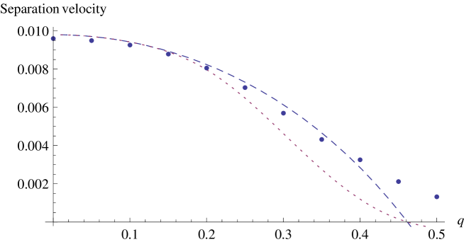
Figure 3: Separation velocity of a pair of spirals 60 units apart using (145) [dashed] and the composite (148) [dotted].

In Figures 2 and 3 we compare the predictions of the canonical, near-field and composite laws of motion with a direct simulation of (1) using second-order accurate finite differences in a square domain of side 800. The figures show the separation and rotation velocity of a pair of $n_{\ell}=1$ spirals when they are separated by a distance 60.

We see that the multiplicative composite expansion captures the qualitative behaviour very well, and provides a reasonable quantitative prediction.

Acknowledgements

M. Aguareles was supported in part by the MEC of Spain, grant MT2005-07660-C02-01. The authors would like to acknowledge many helpful discussions with Prof T Witelski, who performed the numerical simulations reported in §6.

Appendix A Extension to non-zero $b$

For clarity throughout we have only considered the case $b=0$. However, the extension to general values of $b$ does not introduce any further conceptual difficulty, it merely complicates some of the algebra. We indicate here briefly the necessary steps in the calculation.

The outer equation for nonzero $b$ reads

$$\epsilon^{2}(1-ib)\mu\psi_{T}=\epsilon^{2}\nabla^{2}\psi+(1+iq)(1-|\psi|^{2})\psi-\frac{i\epsilon^{2}\alpha^{2}}{q}\psi,$$ (151)

which in terms of modulus $f$ and phase $\chi$ becomes

$$\mu\epsilon^{2}(f_{T}+bf\chi_{T}) =\epsilon^{2}\nabla^{2}f-\epsilon^{2}f|\nabla\chi|^{2}+(1-f^{2})f,$$ (152)

$$\mu\epsilon^{2}(f^{2}\chi_{T}-bff_{T}) =\epsilon^{2}\nabla\cdot(f^{2}\nabla\chi)+qf^{2}(1-f^{2})-\epsilon^{2}\frac{\alpha^{2}}{q}f^{2}.$$ (153)

Upon expanding $\chi$ and $f$ in powers of $\epsilon$ we find that the leading-order terms satisfy

$$f_{0} =1,$$

$$\mu\chi_{0T} =\nabla^{2}\chi_{0}+q|\nabla\chi_{0}|^{2}-\alpha^{2}/q.$$

where the parameter $b$ does not appear; thus the rest of the outer calculation is identical to that of §4.1.

For $b\not=0$, the inner equations close to the $\ell$-th vortex are given by

$$\epsilon\mu\big{(}\epsilon f_{T}-\frac{d{\bf X}_{\ell}}{dT}\cdot\nabla f +\epsilon bf\chi_{T}-bf\frac{d{\bf X}_{\ell}}{dT}\cdot\nabla\chi\big{)},$$

$$=\nabla^{2}f-f|\nabla\chi|^{2}+(1-f^{2})f$$ (154)

$$\epsilon\mu\big{(}b\frac{d{\bf X}_{\ell}}{dT}\cdot f\nabla f-\epsilon bff_{T} +\epsilon f^{2}\chi_{T}-f^{2}\frac{d{\bf X}_{\ell}}{dT}\cdot\nabla\chi\big{)}$$

$$=\nabla\cdot(f^{2}\nabla\chi)+q(1-f^{2})f-\frac{\epsilon^{2}\alpha^{2}}{q}.$$ (155)

Expanding in powers of $\epsilon$ we find that at leading order

$$0=\nabla^{2}\psi_{0}+(1+iq)\psi_{0}(1-|\psi_{0}|^{2}),$$ (156)

while at first order

$$-\mu(1-ib)\frac{d{\bf X}_{\ell}}{dT}\cdot\nabla\psi_{0}=\nabla^{2}\psi_{1}+(1+iq)(\psi_{1}(1-|\psi_{0}|^{2})-\psi_{0}(\psi_{0}\psi_{1}^{*}+\psi_{0}^{*}\psi_{1})),$$ (157)

or equivalently,

$$-\mu\frac{d{\bf X}_{\ell}}{dT}\cdot(\nabla f_{0}+bf_{0}\nabla\chi_{0}) = \nabla^{2}f_{1}-f_{1}|\nabla\chi_{0}|^{2}-2f_{0}\nabla\chi_{0}\cdot\nabla\chi_{1}+f_{1}-3f_{0}^{2}f_{1},$$ (158)

$$-\mu\frac{d{\bf X}_{\ell}}{dT}\cdot(f_{0}^{2}\nabla\chi_{0}-bf_{0}\nabla f_{0}) = \nabla\cdot(f_{0}^{2}\nabla\chi_{1})+\nabla\cdot(2f_{0}f_{1}\nabla\chi_{0})+2qf_{0}f_{1}-4qf_{0}^{3}f_{1}.\qquad$$ (159)

Writing these in terms of the outer variable to find the outer limit of the first order inner, and expanding in $\epsilon$ as $\chi_{1}\sim\widehat{\chi}_{10}(q)/\epsilon+\widehat{\chi}_{11}(q)+\cdots$ and $f_{1}\sim\widehat{f}_{10}(q)+\epsilon\widehat{f}_{11}(q)+\cdots$ as in §4.3.4, we find the equation for $\widehat{\chi}_{10}$ is now given by

$$-\mu\frac{d{\bf X}_{\ell}}{dT}\cdot\nabla\widehat{\chi}_{00}=\nabla^{2}\widehat{\chi}_{10}-2q\widehat{f}_{11}=\nabla^{2}\widehat{\chi}_{10}+2q\nabla\widehat{\chi}_{00}\cdot\nabla\widehat{\chi}_{10},$$ (160)

which again does not involve $b$. Thus the matching between inner and outer solutions is the same as in §4.

Finally we must derive the law of motion when $b$ is not zero. To do so we start by defining the same inner product as before and consider the first order linear operator given in (157), which is of the form

$$L(q,\psi_{0})[\psi_{1}]=w(\psi_{0},q,\mu,b,d{\bf X}_{\ell}/dT)$$

where $L$ does not depend on $b$ but where the non-homogeneous term is now

$$w(\psi_{0},q,\mu,b,d{\bf X}_{\ell}/dT)=-\mu(1-ib)\frac{d{\bf X}_{\ell}}{dT}\cdot\nabla\psi_{0}.$$

Since the linear operator $L$ is the same that that in §4, the only place where $b$ has an effect is in the solvability condition itself, which is obtained through the Fredholm Alternative. The new solvability condition is

$$-\int_{D}\Re\left\{\mu(1-ib)\frac{d{\bf X}_{\ell}}{dT}\cdot\nabla\psi_{0}v^{*}\right\}dD=\int_{\partial D}\Re\left\{(1-iq)\left(v^{*}\frac{\partial\psi_{1}}{\partial n}-\frac{\partial v^{*}}{\partial n}\psi_{1}\right)\right\}dl.$$ (161)

Since the left-hand side is $O(\mu)$, a nonzero value of $b$ does not affect the velocity law at leading order, but it will alter the $O(\mu)$ correction terms.

Figure 1: The velocity of rotation of a pair of $+1$ spirals as a function of $q$ for $\epsilon=1/20$ and $|{\bf X}_{1}-{\bf X}_{2}|=2$ using the formulae for the canonical scaling (solid), the near-field scaling (dashed), the additative composite (dotted) and the multiplicative composite (dot-dashed). We see that the multiplicative composite is likely to be a much better approximation, especially for $q>\pi/2\log|\epsilon|$.

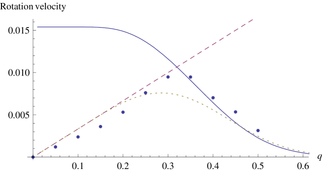
Figure 2: Rotation velocity of a pair of spirals 60 units apart as a function of $q$, using (143) [solid], (145) [dashed] and the composite (148) [dotted]. The points correspond to a numerical simulation of (1).

References

- [1] M. Aguareles, S. J. Chapman, and T. Witelski. Interaction of spiral waves in the complex ginzburg-landau equation. Phys. Rev. Lett., 101:art. no. 224101, 2008.
- [2] I. Aranson, L. Kramer, and A. Weber. Theory of interaction and bound states of spiral waves in oscillatory media. Phys. Rev. E, 47(4):3231–3241, 1993.
- [3] I. S. Aranson and L. Kramer. The world of the complex Ginzburg-Landau equation. Rev. Modern Phys., 74(1):99–143, 2002.
- [4] S. J. Chapman and G. Richardson. Motion of vortices in type II superconductors. SIAM J. Appl. Math., 55(5):1275–1296, 1995.
- [5] S. J. Chapman and G. Richardson. Vortex pinning by inhomogeneities in type-II superconductors. Phys. D, 108(4):397–407, 1997.
- [6] J. Greenberg. Spiral waves for systems. SIAM J. Appl. Math., 39(2):301–309, 1980.
- [7] P. S. Hagan. Spiral waves in reaction-diffusion equations. SIAM J. Appl. Math., 42(4):762–786, 1982.
- [8] J. V. Moloney and A. C. Newell. Nonlinear optics. Phys. D, 44(1-2):1–37, 1990.
- [9] J. C. Neu. Vortices in complex scalar fields. Phys. D, 43(2-3):385–406, 1990.
- [10] L. Peres and J. Rubinstein. Vortex dynamics in Ginzburg-Landau models. Phys. D, 64(1-3):299–309, 1993.
- [11] L. M. Pismen. Weakly radiative spiral waves. Phys. D, 184(1-4):141–152, 2003. Complexity and nonlinearity in physical systems (Tucson, AZ, 2001).
- [12] L. M. Pismen and A. A. Nepomnyashchy. On interaction of spiral waves. Phys. D, 54(3):183–193, 1992.
- [13] M. Van Dyke. Perturbation Methods in Fluid Mechanics. Parabolic Press, Stanford, CA, 1975.
- [14] R. W. Walden, P. Kolodner, A. Passner, and C. M. Surko. Traveling waves and chaos in convection in binary fluid mixtures. Phys. Rev. Lett., 55(5):496–499, Jul 1985.