GRS 1915+105 in “Soft State”: Nature of Accretion Disk Wind and Origin of X-Ray Emission

Abstract

We present the results from simultaneous Chandra HETGS and RXTE observations of the microquasar GRS 1915+105 in its quasi-stable “soft state” (or State A) performed on 2007 August 14, several days after the state transition from “hard state” (State C). The X-ray flux increased with spectral hardening around the middle of the Chandra observation, after which the 67 Hz quasi periodic oscillation (QPO) became significant. The HETGS spectra reveal at least 32 narrow absorption lines from highly ionized ions including Ne, Mg, Si, S, Ar, Ca, Cr, Mn, Fe, whose features are the deepest among those ever observed with Chandra from this source. By fitting to the absorption line profiles by Voigt functions, we find that the absorber has outflow velocities of $\approx$150 and $\approx$500 km s^-1 with a line-of-sight velocity dispersion of $\approx$70 and $\approx$200 km s^-1 for the Si XIV and Fe XXVI ions, respectively. The larger velocity and its dispersion in heavier ions indicate that the wind has a non-uniform dynamical structure along the line-of-sight. The location of the absorber is estimated at $\sim(1-3)\times 10^{5}r_{\rm g}$ ($r_{\rm g}$ is the gravitational radius) from the source, consistent with thermally and/or radiation driven winds. By taking into account narrow spectral features detected with Chandra, the continuum spectra obtained with RXTE in the 3–25 keV band can be well described with a thermal Comptonization with an electron temperature of $\approx 4$ keV and an optical depth of $\approx 5$ from seed photons from the standard disk extending down to $(4-7)r_{\rm g}$. In this interpretation, most of the radiation energy is produced in the Comptonization corona, which completely covers the inner part of the disk. A broad ($1\sigma$ width of $\approx 0.2$ keV) iron-K emission line and a smeared edge feature are detected, which can be explained by reflection from the accretion disk at radii larger than $400r_{\rm g}$. Our data do not require the presence of an extremely blurred iron-K line or disk emission originating from radii smaller than $\approx 4r_{\rm g}$ in this state.

1. Introduction

Microquasars are key objects to investigate the physics of accretion onto a black hole in relation with relativistic jet. GRS 1915+105 is the most important, archetype microquasar, from which the first superluminal motion in our Galaxy was detected (for review, see Fender & Belloni, 2004). It is an X-ray binary consisting of a M-K III star and a black hole of $14\pm 4$ ${\rm M_{\odot}}$with an inclination angle of 66^∘–70^∘ at a distance of $\approx 12$ kpc. The luminosity of GRS 1915+105 reaches close to the Eddington limit, indicating critical mass accretion takes place. With this reason, GRS 1915+105 exhibits unique properties distinct from canonical black hole binaries (BHBs). In particular, it sometimes shows dramatic temporal/spectral variations (“oscillation”) occurring in quasi-regular cycles, most probably due to thermal instability in the accretion disk. Belloni et al. (2000) phenomenologically classified the X-ray states into three, States A, B, and C. GRS 1915+105 spends most of time in State C where the X-ray spectrum is relatively hard. The underlying physics of these complex behaviors and the relation to canonical BHBs is far from being fully understood, even though it is a key question to establish a general solution of accretion onto black holes at various mass accretion rates.

Outflow by a disk wind is one of key ingredients in understanding the dynamics of an accretion flow in disk systems, including X-ray binaries and active galactic nuclei. Kotani et al. (2000) discovered absorption line features of iron-K ions in the X-ray spectra of GRS 1915+105 with ASCA, revealing the presence of a significant amount of highly ionized plasma in this system. Similar features were reported in many other X-ray binaries including both black holes (e.g., Ueda et al., 1998; Miller et al., 2006) and neutron stars (e.g., Ueda et al., 2001; Boirin et al., 2004), which are now recognized to be a common feature in accreting sources over a wide range of luminosity. The origin of such ionized gas has been established to be a disk wind by the precise measurement of the outflow velocity with Chandra. The physical mechanism to produce the disk wind is not established yet. There are at least 3 possibilities that are not exclusive one another: thermally-driven wind (Begelman et al., 1983), radiation driven wind (e.g., Proga, Stone, & Kallman, 2000), and/or magnetically driven wind. Based on a simple argument from an observed column density and an ionization parameter, the location of the wind has been estimated at $10^{4-5}r_{\rm g}$ ($r_{\rm g}\equiv GM/c^{2}$ is the gravitational radius where $G$, $M$, $c$ is the gravitational constant, mass of the black hole, and light velocity, respectively.) from the source, consistent with thermally and/or radiation driven in all the cases (including GRO J1655–40) except for Miller et al. (2006), who deduced a much smaller radii from Chandra data of GRO J1655–40, leading to their conclusion that a magnetically driven wind is the only solution. This argument is questioned by Netzer (2006), however, making the discussion still controversial.

Detailed studies of the disk wind in GRS 1915+105 is particularly important to understand the role and origin of the outflow at high mass accretion rates. Among the different epochs observed with ASCA, the absorption features were the most prominent (equivalent widths of 30–50 eV for H- and He-like Fe ions) in 1994 and 1995 when the spectrum is soft and the 1–10 keV flux is relatively faint ($\sim$0.3 Crab). We recognize that in these ASCA observations the source was in quasi-stable “soft state” (State A), which is found to be quite rare case in the long term variability from the RXTE/ASM over $>$10 years. By contrast, the iron-K absorption-line features were much weaker and even undetectable when the 1–10 keV spectrum was hard, corresponding to State C (or “hard state”). This can be explained by the increasing photon flux responsible for photo-ionization which almost fully ionized the ions. Lee et al. (2002) performed a HETGS observation of GRS 1915+105 in State C and detected absorption lines from highly ionized Fe ions. However, the features are much weaker, with equivalent widths of only  10 eV, compared with those found in State A with ASCA. Because of the weakness of these features there still remain uncertainties in the basic properties of the plasma, such as the bulk velocity and its dispersion (or kinetic temperature).

In this paper, we report the results of high energy resolution spectroscopy of GRS 1915+105 in “soft state” (State A) performed simultaneously with Chandra HETGS and RXTE in 2007 August. The first purpose is to reveal the origin of the disk wind with the best spectroscopic data ever obtained for absorption-line diagnostics of the highly ionized plasma in GRS 1915+105. Secondly, we study the origin of the continuum emission in this state by utilizing the ideal combination of Chandra and RXTE. The simultaneous HETGS data enable us to take into account all the spectral features in the analysis of the RXTE PCA spectra, including interstellar/circumstellar absorptions with anomalous metal abundances, narrow absorption lines by highly ionized gas, and a broad iron-K emission line. § 2 summarizes the observations and data reduction. The results and discussion are presented in § 3 and § 4, respectively. We assume the distance toward GRS 1915+105 of 12.5 kpc and the inclination of 70^∘ throughout the paper. Quoted errors for spectral parameters are 90% confidence level for a single parameter unless otherwise mentioned. Multiwavelengths properties of GRS 1915+105 including radio and infrared data over a long period covering our observation are presented by Arai et al. (2008).

2. Observations and Data Reduction

2.1. Chandra Data

The Chandra HETGS observation of GRS 1915+105 was carried out from 2007 August 14 5:22 (UT) to 19:35 for an exposure of 47.4 ksec as a target-of-opportunity (ToO) observation (obsID 7485). Figure 1 shows the long term light curves of GRS 1915+105 monitored by the RXTE ASM in the 2–12 keV band, its hardness ratio $HR2$ between the 5–12 keV and 3–5 keV bands, and that by Swift BAT in the 15–50 keV band. To catch the source in “soft state”, we set the trigger condition for the Chandra ToO that the following two criteria holds for 2 or more successive days: (1) the ASM count rate $<30$ c/s and (2) $HR2<1.1$. As seen from the figure, GRS 1915+105 made a state transition around 2007 August 8, entering into a quasi-stable “soft state” where the 15–50 keV flux became below the detection limit of the BAT. The position of the arrows denote our observation epoch. To make the effects of pile-up least, we adopt graded telemetry mode and readout only one-third of the full frame using a subarray. We did not use ACIS-S0 and S5, because GRS 1915+105 is heavily absorbed and has little photons below $\sim$ 1 keV.

Figure 1.— Upper: the long term light curve of GRS 1915+105 observed with the RXTE ASM. Middle: the hardness ratio ($HR2$) of the RXTE ASM count rates between 5–12 keV and 3–5 keV bands. Lower: Swift BAT light curve in the 15–50 keV band. The epoch of our observations is denoted by the arrows. The dashed lines correspond to 30 cts/s (upper) and $HR2=1.1$ (middle), thresholds for triggering our ToO observations aiming at the “soft” state.

We reduce the data using the CIAO version 3.4 and the CALDB version 3.4.5 provided by the Chandra X-ray Center (CXC). To determine the zero-th order position most accurately under heavy pile-up, we utilize the tg_findzo script. The accuracy of relative wavelengths calibration of the HETGS is 0.05 pixel in position within a chip , corresponding to 0.00028 $\AA$ in the HEG (or, 14 km s^-1 at 2 keV and 47 km s^-1 at 7 keV), although the accuracy may be worse if we use the data over multiple chips, because of a chip-gap error (Marshall, H., private communication). As described below, we are particularly interested in the energy determination in the 2.0–7.0 keV range (between the $K\alpha$ lines from Si XIV and Fe XXVI), which is covered within a single chip in the $-1$ order spectrum. We confirm that the $+1$ data give consistent results with the $-1$ one. Thus, velocity difference between Si XIV and Fe XXVI ions can be measured within an accuracy of $<$50 km s^-1.

In this paper we mainly utilize the 1st-order HEG data, which cover energies above 4 keV and has twice better energy resolution than the MEG. For spectra below 1.6 keV, the MEG data are utilized instead, which have about three times larger effective area there. Pile-up is corrected according to the method described in Ueda et al. (2004); we calculate the fractional count rate loss as $f=1-{\rm exp}(-7.5R)$, where $R$ is the count rate of the ACIS pixel in units of count per pixel per frame, and multiply the observed spectra by $1/(1-f)\simeq 1+7.5R$. The correction factor is found to be 15% at maximum around 4–5 keV in the HEG data. The spectra from the $+1$ and $-1$ orders are summed. We conservatively add a systematic error of 3% in each bin of the spectra. The XSPEC package (version 11.3.2) is used for spectral analysis.

2.2. RXTE Data

Following the trigger of the Chandra ToO, Rossi X-ray Timing Explorer (RXTE) performed two ToO observations of GRS 1915+105 at 2007 August 14 07:36–08:57 (Epoch I’) and 17:00–18:03 (Epoch II’) during the Chandra observation. RXTE carries two pointing instruments, the Proportional Counter Array (PCA: Jahoda et al. 2006) and the High Energy Timing Experiment (HEXTE: Rothschild et al. 1998). We only analyze the PCA data in this paper, because the spectra of GRS 1915+105 were very soft in our observations and hence the HEXTE data do not give strong constraints. The HEADAS package (version 6.4) is used for the analysis. The data are selected by the following criteria: 1) RXTE was not in the South Atlantic Anomaly, 2) the elevation angle was below 10 degrees, and 3) the offset angle between the pointing direction and the target was less than 0.02 degree. The net exposures are 2.4 ksec and 3.2 ksec for Epochs I’ and II’, respectively.

We utilize the “standard 2” PCA data for spectral analysis, which have 16 sec time resolution and 129 energy channels. We extract energy spectra from the data of the top layer of Proportional Counter Unit (PCU) 2, the best calibrated one. The background is subtracted using the model applicable for bright sources. The deadtime, about 3–4%, is corrected. A systematic error of 1.5% is added for each energy channel. To check the calibration accuracy, we also analyze the spectra of Crab Nebula observed on 2007 August 11. We confirm that the combined PCU 2 and HEXTE (Cluster-B) spectra in the 3.5–200 keV band are well reproduced by a single power-law with a photon index of 2.07$\pm$0.01 for a fixed Galactic absorption of $N_{\rm H}=3\times 10^{21}$ cm^-2. The flux in the 3–20 keV band determined by PCU 2 is 2.63$\times$10^-8 ergs cm^-2 s^-1, which is consistent within 10% of the nominal value (Toor & Seward, 1974).

For timing analysis of the PCA, we use two types of single-bit data covering the energy range of 3.2–5.6 keV and 5.6–14.8 keV, and event-mode data covering energies above 14.8 keV. They have a time resolution of 122 $\mu$s (single bit) and 16 $\mu$s (event mode), respectively. The light curves from these data are co-added to produce one light curve in the 3.2–37.9 keV band. The power spectral density (PSD) is then calculated by the powspec ftool in the XRONOS package. It is known that the PSD computed from PCA data in the Leahy normalization is less than 2, a value expected from Poisson distribution, at high frequencies above 10 Hz due to deadtime effects (Zhang et al., 1995). We thus subtract the dead-time corrected Poisson noise level from the observed PSD, following the method by Morgan, Remillard, & Greiner (1997).

3. Results

3.1. Light Curves and Power Spectra

Figure 2 shows the light curves of GRS 1915+105 with 16 sec resolution obtained with the Chandra HETGS in the 1–8 keV band (upper panel), RXTE PCA in the 3.2–38 keV band (middle), and the hardness ratio between the 5.6–38 keV and 3.2–5.6 keV PCA count rates (lower). In the upper panel, we plot the sum of the MEG and HEG count rates including the 1st, 2nd, and 3rd orders. As noticed from the figure, the averaged flux level was roughly constant in the first half and then started to increase from the middle of the observation, accompanied with spectral hardening. The PCU2 count rate increased by about $70\%$ in the latter observation. It is also seen that the flux is highly variable on a shorter time scale than $10^{4}$ sec. For later discussion, we divide the epoch into two, Epoch I (before 2007 August 14 13:06:40) and Epoch II (after). We refer the two intervals of the RXTE observations as Epoch I’ (former) and II’ (latter). These observations would be classified as “$\phi$” (steady State A) in the nomenclature of Belloni et al. (2000), since the hardness ratio values are low, there is limited variability, and there is no structure in the color-color diagram (not shown). During Epoch II, the count rate approaches the level that is more typical of the “$\delta$” class, where there are transitions between States A and B, and hence Epoch II can be considered to be an interval of “bright $\phi$” conditions.

Figure 2.— Upper: the Chandra HETGS light curve (sum of the HEG 1st, 2nd, and 3rd order events) with a time resolution of 16 sec. No correction is made for pile-up. Middle: RXTE PCA light curve in the 3.2–38 keV band with a time resolution of 16 sec (only PCU2 data are utilized). Lower: the PCA hardness ratio between the 5.6–38 keV and 3.2–5.6 keV bands.

The power spectral density in the 3–38 keV band calculated from the RXTE PCA is shown in Figure 3. While there are no clear QPO features in Epoch I’, a QPO is detected at 66.8$\pm$1.1 Hz at 4.3$\sigma$ level in Epoch II’. The coherence parameter in this QPO is $Q=\nu_{0}/{\rm FWHM}\approx 11$, where $\nu_{0}$ is the central QPO frequency and the fit uses a Lorentzian profile. We note that the difference in the QPO intensity between the two epochs is not highly significant, however. The integrated fractional root mean square around the 67 Hz QPO is found to be 0.8%$\pm$0.4% and 1.6%$\pm$0.2% in Epoch I’ and II’, respectively (the errors are 1$\sigma$).

Figure 3.— The normalized power spectral density in Epochs I’ (upper) and II’ (lower) obtained from the RXTE PCA data covering the 3.2–38 keV band. The Poisson noise level was subtracted after dead time correction. The position of the 67 Hz QPO is denoted by the arrow.

3.2. HETGS Spectra

Figure 4 shows the HETGS spectra integrated over the whole observation. Here we only correct the spectrum for effective area as a function of energy, but not for the instrumental energy resolution, which is 3.2 eV at 2.0 keV and 40 eV at 7.0 keV in the HEG. The MEG data are utilized in the 1.0–1.6 keV band, while the HEG data for the rest. Although the overall spectral shape changed from Epoch I to II as mentioned above, we first study this spectrum as the base data from which we can best constrain local spectral features in time-averaged sense. We find that the overall continuum can be well described by a cutoff power law model, expressed as $A\;E^{-\Gamma}{\rm exp}(-E/E_{\rm fold})$, subject to heavy interstellar absorption with non-solar abundances. The best-fit parameters are summarized in Table 1. Note that the cutoff power law model is only empirical and does not have physical meaning itself; we will model the continuum emission by physical models for the PCA spectra in § 3.3.

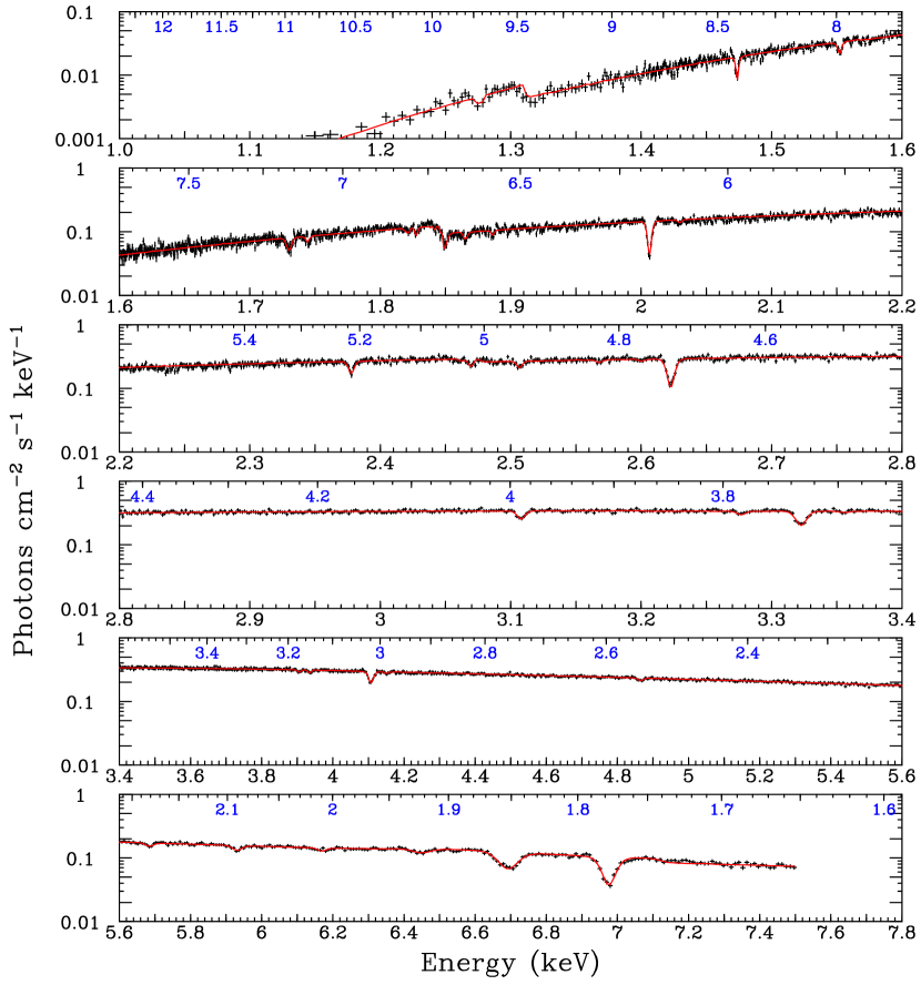
Figure 4.— The Chandra HETGS spectrum integrated over the whole observation (corrected for the effective area but not for the energy resolution). From upper to lower: 1.0–1.6 keV, 1.6–2.2 keV, 2.2–2.8 keV, 2.8–3.4 keV, 3.4–5.6 keV, 5.6–7.8 keV. The HEG 1st-order events are used except below 1.6 keV, where the MEG 1st-order data are utilized. The solid curve (red) represents the best-fit continuum (modelled by an absorbed cutoff power law) modified by absorption lines (negative gaussians) and a broad iron-K emission (a positive gaussian). The upper axis of each panel marks wavelengths in units of Å (blue).

Table 1Spectral Parameters of the Time-averaged HETGS Spectrum

Parameter	Best-fit
Column Densities ($N_{\rm H}$)
H ($10^{22}$ cm-2)	2.78$\pm$0.03
Mg ($10^{22}$ cm-2)	6.3$\pm$1.4
Si ($10^{22}$ cm-2)	5.8$\pm$0.4
S ($10^{22}$ cm-2)	7.6$\pm$1.2
Fe ($10^{22}$ cm-2)	10$\pm$1
Continuum
$A$	7.15$\pm$0.25
$\Gamma$	1.17$\pm$0.06
$E_{\rm fold}$ (keV)	3.80$\pm$0.17
Iron-K Emission Line
$E_{\rm cen}$ (keV)	6.55$\pm$0.04
1$\sigma$ width (keV)	0.17$\pm$0.04
E.W. (eV)	45$\pm$8
$E_{\rm cen}$ (keV)	6.54$\pm$0.03
1$\sigma$ width (keV)	0.05 (fixed)
$r_{\rm in}$ ($r_{\rm g}$)	600${}^{+300}_{-200}$
$r_{\rm out}$ ($r_{\rm g}$)	$100000$ (fixed)
$\beta$	$-3$ (fixed)

Note. — The errors are 90% confidence level for a single parameter.

It is a critical issue to accurately determine the column densities of major elements in the interstellar (plus circumstellar) matter toward GRS 1915+105 for detailed study of its spectral model. In spectra with insufficient energy resolution, a deep absorption edge produced by interstellar matter can be coupled with other spectral features such as emission lines at similar energies. It could also affect the continuum shape at low energies where the photo-electronic absorption cross section is large. The Chandra high resolution data provide us with the best opportunity to solve this issue for this source. The result also has an important implication for study of elemental abundances in the Galaxy, although we do not discuss it here. Lee et al. (2002) determined column densities of Mg, Si, S, and Fe by measuring the K-edge depth of each element, which are quite useful and are adopted by some authors for spectral modelling (e.g., Done et al., 2004).

In this paper, we re-determine those values from our data that have a better statistics than that of Lee et al. (2002), following the same method described in Ueda et al. (2005). We adopt the photo-electric absorption cross section by Wilms et al. (2000), which is available as TBvarabs model in XSPEC. The column density of lighter elements than Mg is determined by a spectral fit to the whole continuum. Here we consider the effect of dust scattering based on the cross section by Draine (2003). Those of other elements are locally fit around the K-edge by taking into account X-ray absorption fine structure (XAFS); in particular, it is difficult to accurately estimate the column density of Si just by measuring a depth of Si-K edge, due to the complicated XAFS that is most likely attributed to silicates grains. We thus model it using an experimental cross section of SiO₂ as done in Ueda et al. (2005). Table 1 lists the Hydrogen-equivalent column densities of each element assuming the solar abundances by Anders & Grevesse (1989) for each element, which are used in our subsequent analysis at their best-fit values. The relative abundances within the groups of H-He-C-N-O, Ne-Na-Mg-Al, S-Cl-Ar-Ca, and Cr-Fe-Co-Ni are fixed at the solar values. We find the column density of Si is not as large as that estimated by Lee et al. (2002). For the column density of Fe, we adopt a value determined with Suzaku (Ueda, Y. et al. in preparation) because the Chandra result has a large statistical error, yet consistent with the Suzaku result, due to the limited energy coverage and area above 7.1 keV.

As seen from Figure 4, we detect 33 narrow absorption lines over the whole energy range of HETGS, for which we simply model with negative gaussians in the plot. We find that 32 of them correspond to transition in highly ionized (H-like or He-like) ions. The absorption line at 2.470 keV, identified as S II, is most probably produced by interstellar matter in the Galaxy, which is commonly seen in the high resolution spectra of Galactic sources (Ueda et al., 2005). The energy, 1$\sigma$ width, and equivalent widths are listed in Table 2 with its identification. For weak lines whose width cannot be well determined, we assume a velocity dispersion of 100 km s^-1 or 200 km s^-1, depending on element. In addition to those narrow absorption lines, a broad emission line feature centered at 6.55$\pm$0.04 keV is found, attributable to K$\alpha$ lines of mildly ionized Fe ions. This can be modeled by a single broad ($1\sigma$ width of 0.17$\pm$0.04 keV) gaussian or by a narrower (0.05 keV) gaussian blurred with the “disk line” profile (Fabian et al., 1989), which is a more physical interpretation for an iron-K line from the accretion disk (see § 4.2 for discussion). In the disk-line fit, we assume an outer radius of $10^{5}r_{\rm g}$ with an emissivity law of $r^{\beta}$ where $r$ is the radius and $\beta=-3$, and make the center energy and inner radius as free parameters. The parameters of the emission line are summarized in Table 1.

Table 2List of Absorption Lines Observed in the HETGS spectra

$E_{\rm obs}$	$1\sigma$ width	E.W.	line ID	$E_{\rm theory}$ (term of final state)
(keV)	(eV)	(eV)		(keV)
1.277(4)	0.43*	1.8	Ne X 4p	1.27707 (${}^{2}P_{1/2}$), 1.27713 (${}^{2}P_{3/2}$)
1.4734(4)	0.001($<1.0$)	1.7	Mg XII 2p	1.47169 (${}^{2}P_{1/2}$), 1.47264 (${}^{2}P_{3/2}$)
1.5522(6)	1.0(8)	1.4	Fe XXIV 2s$\rightarrow$4p	1.55091 (${}^{2}P_{1/2}$), 1.55289 (${}^{2}P_{3/2}$)
1.7301(7)	2(1)	1.9	Al XIII 2p	1.72769 (${}^{2}P_{1/2}$), 1.72899 (${}^{2}P_{3/2}$)
			Fe XXIV 2s$\rightarrow$5p	1.72876 (${}^{2}P_{1/2}$), 1.72978 (${}^{2}P_{3/2}$)
1.7456(9)	0.04($<1.1$)	0.67	Mg XII 3p	1.74456 (${}^{2}P_{1/2}$), 1.74484 (${}^{2}P_{3/2}$)
1.818(2)	0.61*	0.31	Ni XXVI 2s$\rightarrow$4p	1.81758 (${}^{2}P_{1/2}$), 1.82033 (${}^{2}P_{3/2}$)
1.8276(5)	0.61*	0.75	Fe XXIV 2s$\rightarrow$6p	1.82640 (${}^{2}P_{1/2}$), 1.82698 (${}^{2}P_{3/2}$)
1.842(2)	0.61*	0.54	Mg XII 4p	1.84002 (${}^{2}P_{1/2}$), 1.84014 (${}^{2}P_{3/2}$)
1.8861(8)	0.63*	0.49	Mg XII 5p	1.88419 (${}^{2}P_{1/2}$), 1.88426 (${}^{2}P_{3/2}$)
2.0063(3)	1.4(2)	3.4	Si XIV 2p	2.00433 (${}^{2}P_{1/2}$), 2.00608 (${}^{2}P_{3/2}$)
2.029(2)	0.68*	0.39	Ni XXVI 2s$\rightarrow$5p	2.02775 (${}^{2}P_{1/2}$), 2.02916 (${}^{2}P_{3/2}$)
2.3777(5)	0.7($<1.8$)	1.7	Si XIV 3p	2.37611 (${}^{2}P_{1/2}$), 2.37663 (${}^{2}P_{3/2}$)
2.460(4)	0.82*	0.54	S XV 2p	2.46063 (${}^{1}P_{1}$)
2.470(1)	2(1)	1.3	S II 3p	2.4694
2.507(1)	0.83*	1.2	Si XIV 4p	2.50616 (${}^{2}P_{1/2}$), 2.50638 (${}^{2}P_{3/2}$)
2.568(3)	0.85*	0.46	Si XIV 5p	2.56632 (${}^{2}P_{1/2}$), 2.56644 (${}^{2}P_{3/2}$)
2.599(4)	0.87*	0.44	Si XIV 6p	2.59899 (${}^{2}P_{1/2}$), 2.59906 (${}^{2}P_{3/2}$)
2.6229(3)	2.5(3)	5.2	S XVI 2p	2.61970 (${}^{2}P_{1/2}$), 2.62270 (${}^{2}P_{3/2}$)
3.1077(7)	0.9(${}^{+1.4}_{-0.8}$)	2.0	S XVI 3p	3.10586 (${}^{2}P_{1/2}$), 3.10675 (${}^{2}P_{3/2}$)
3.277(2)	1.1*	0.92	S XVI 4p	3.27589 (${}^{2}P_{1/2}$), 3.27627 (${}^{2}P_{3/2}$)
3.3227(6)	2.9(7)	4.5	Ar XVIII 2p	3.31818 (${}^{2}P_{1/2}$), 3.32299 (${}^{2}P_{3/2}$)
3.355(4)	1.1*	0.44	S XVI 5p	3.35454 (${}^{2}P_{1/2}$), 3.35473 (${}^{2}P_{3/2}$)
3.905(4)	1.3*	1.1	Ca XIX 2p	3.90226 (${}^{1}P_{1}$)
3.937(4)	1.3*	1.2	Ar XVIII 3p	3.93429 (${}^{2}P_{1/2}$), 3.93572 (${}^{2}P_{3/2}$)
4.1070(8)	5(2)	6.1	Ca XX 2p	4.10015 (${}^{2}P_{1/2}$), 4.10750 (${}^{2}P_{3/2}$)
4.151(6)	1.4*	0.80	Ar XVIII 4p	4.14974 (${}^{2}P_{1/2}$), 4.15034 (${}^{2}P_{3/2}$)
4.865(5)	1.6*	1.7	Ca XX 3p	4.86192 (${}^{2}P_{1/2}$), 4.86410 (${}^{2}P_{3/2}$)
5.684(6)	3.8**	3.3	Cr XXIII 2p	5.68205 (${}^{1}P_{1}$)
5.931(4)	7($<16$)	5.8	Cr XXIV 2p	5.91650 (${}^{2}P_{1/2}$), 5.93185 (${}^{2}P_{3/2}$)
6.17(2)	4.1**	3.6	Mn XXIV 2p	6.18044 (${}^{1}P_{1}$)
6.45(1)	17(${}^{+14}_{-12}$)	7.9	Mn XXV 2p	6.42356 (${}^{2}P_{1/2}$), 6.44166 (${}^{2}P_{3/2}$)
6.692(3)	28(3)	40	Fe XXV 2p	6.70041 (${}^{1}P_{1}$)
			Fe XXIV 2p	6.67644 (${}^{2}P_{1/2}$), 6.67915 (${}^{2}P_{3/2}$)
6.975(2)	16(2)	40	Fe XXVI 2p	6.95196 (${}^{2}P_{1/2}$), 6.97317 (${}^{2}P_{3/2}$)
			Cr XXIV 3p	7.01726 (${}^{2}P_{1/2}$), 7.02181 (${}^{2}P_{3/2}$)

Note. — The MEG data are utilized for the absorption lines below 1.6 keV.

Note. — The single number in the parenthesis indicates the statistical error in the last digit (90% confidence level for a single parameter).

To determine the physical parameters of the ionized plasma, we next fit the absorption line profile of major elements (Si, S, Ar, Ca, Cr, Mn, Fe) by a Voigt function in the local energy band. The Voigt profile, whose opacity is expressed by a convolution of a gaussian and a lorenzian (natural broadening), is a physically more correct model rather than a negative gaussian. To do this, we utilize a local model (called “Kabs”) implemented on XSPEC as described in Ueda et al. (2004), where its full formula is given. The free parameters are three per each ion, a column density (cm^-2), a line-of-sight velocity dispersion $b$ (km s^-1), and a Doppler shift $z=v/c$, where $v$ is the mean bulk velocity of plasma (negative for outflow) and $c$ is the light velocity. The atomic data are taken from the database provided by National Institute of Standards and Technology (NIST). In this paper, we treat an ideal case where contribution of re-emission line from the plasma out of the line-of-sight is neglected, corresponding to Case I in Ueda et al. (2004) or “non-radiative de-excitation limit” in Masai & Ishida (2004). It is because the contribution of the emission cannot be well constrained by our data, being consistent with zero within the statistical errors; when we include such emission lines emitted at $r=(1-3)\times 10^{5}r_{\rm g}$ with an emissivity law of $r^{-3}$ (corresponding to the case of an optically thin, self-similar flow with a constant velocity) and an inclination of 70^∘ in the spectral model, we obtain an upper limit for the solid angle of the plasma as $\Omega/2\pi<0.11$ (90% confidence level) from a simultaneous fit to the Si XIV and S XVI absorption lines. We find that inclusion of these emission lines at the maximum level could increase the column density obtained for the same velocity dispersion by $\approx$30% for Si XIV and $\approx$50% for Fe XXVI, which are within the statistical errors.

We hereafter analyze the HETGS spectra of Epochs I and II separately, since the absorption line profile could change according to the evolution of the continuum spectrum. Figure 5 shows the HEG 1st-order spectra corrected for effective area (i.e., incident spectra except for blurring with the energy resolution). It is evident that the spectrum is harder in Epoch II than in Epoch I. In this subsection, we focus on the absorption lines. Detailed analysis of the continuum is given in next subsection using the RXTE PCA data, which have a wider energy coverage than the HETGS.

Figure 5.— Upper: The HEG 1st-order spectrum (corrected for effective area) in Epoch I. Lower: The HEG 1st-order spectrum (corrected for effective area) in Epoch II.

To best constrain the physical parameters of each ion, we fit two absorption lines of K$\alpha$ and K$\beta$, whenever available (i.e., except for Mn and Fe), simultaneously in the local bands. This works quite well to de-couple the inevitable anti-correlation between a column density and a velocity dispersion in the curve-of-growth analysis. We simply adopt an absorbed cut-off power model for the continuum by fixing $E_{\rm fold}$ and the interstellar absorption. The velocity dispersion in two epochs is found to be consistent with a constant value within the errors. We thus assume the best-fit velocity dispersion obtained from the summed spectrum of Epochs I and II when deriving the column density and Doppler shift of the Si, S, Ar, and Ca ions in each epoch. In the iron-K band, we simultaneously fit K$\alpha$ and K$\beta$ lines of Cr XXIV, K$\alpha$ of Mn XXV, and K$\alpha$ of Fe XXVI by assuming a same velocity dispersion and Doppler shift. The Cr XXIV K$\beta$ line (7.02 keV) contaminates a high energy part of the Fe XXVI K$\alpha$ feature in the HETGS spectra. We treat the Fe XXV absorption line independently, considering possible uncertainties in the incident line energies and a contamination of less ionized ions such as Fe XXIV, although we assume the same velocity dispersion as that of Cr XXIV, Mn XXV, and Fe XXVI. We note that the results of Fe XXV may not be reliable to be taken at their face values but just provide a rough estimate. For Si XIV and Fe XXVI, we introduce an upper limit for the column density constrained by the corresponding K-edge depth measured by HETGS and by PCA, respectively; otherwise, the fit to the absorption line profile leads to unphysically large column densities.

Figure 6 shows a blow-up of absorption line profile in Epochs I and II for each set of elements around their K$\alpha$ lines. The solid curves represent the best-fit model. Table 3 gives the summary of the parameters. We find that all the ions have significant blue shifts, $\approx$150 km s^-1 for Si XIV and $\approx$500 km s^-1 for Fe XXVI. The difference of the velocity between H-like Si (and S, Ar, Ca) and Fe ions is robust, larger than the systematic error in the relative wavelength calibration as mentioned in § 2.1. The velocity dispersion increases with the atomic number, from 70 km s^-1 for Si to $\approx$ 200 km s^-1 for Fe. From Epoch I to II, the column density of all the ions decreases, indicating that the plasma was in a higher ionization stage in the latter epoch than the former; the number ratio between Fe XXV and Fe XXVI is also consistent with this picture.

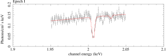
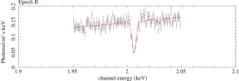
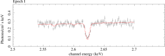
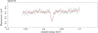
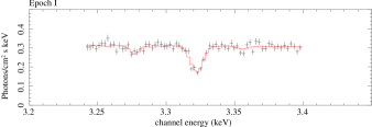
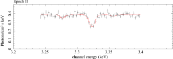
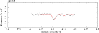
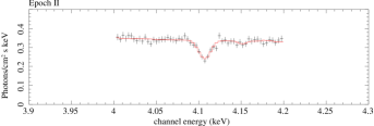
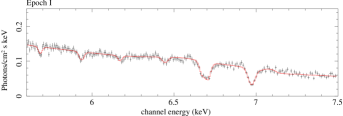
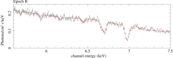
Figure 6.— A blowup of the time-averaged HEG 1st-order spectra around each K-absorption line in Epochs I (left) and II (right). The best-fit model employing Voigt functions is plotted with a line (red). From upper to lower: Si XIV, S XVI, Ar XVIII, Ca XX, Cr XXIV + Mn XXV + Fe XXV + Fe XXVI.

Table 3Parameters of the K$\alpha$ Absorption Lines Fit by Voigt Profile

	Epoch I				Epoch II
Ions	$-z$	$b$	$N_{\rm ion}$		$-z$	$b$	$N_{\rm ion}$
	($\times 10^{-3}$)	(km s-1)	($10^{18}$ cm-2)		($\times 10^{-3}$)	(km s-1)	($10^{18}$ cm-2)
Fe XXVI	$1.68\pm 0.18$	190${}^{+40}_{-30}$	13${}^{+7}_{-8}$		$1.72^{+0.09}_{-0.05}$	210$\pm 10$	10${}^{+0}_{-3}$
Fe XXV	$0.66\pm 0.07$	(= Fe XXVI)	7.2$\pm 1.4$		$0.31\pm 0.08$	(= Fe XXVI)	2.2$\pm 0.3$
Mn XXV	(= Fe XXVI)	(= Fe XXVI)	0.19$\pm 0.06$		(= Fe XXVI)	(= Fe XXVI)	0.16$\pm 0.06$
Cr XXIV	(= Fe XXVI)	(= Fe XXVI)	0.19$\pm 0.04$		(= Fe XXVI)	(= Fe XXVI)	0.12$\pm 0.05$
Ca XX	$0.61^{+0.13}_{-0.19}$	110${}^{+300}_{-20}$*	0.31${}^{+0.12}_{-0.06}$		$0.63^{+0.17}_{-0.54}$	(= Epoch I)*	0.18${}^{+0.04}_{-0.05}$
Ar XVIII	$0.41^{+0.10}_{-0.13}$	110${}^{+170}_{-40}$*	0.26$\pm 0.05$		$0.62^{+0.20}_{-0.15}$	(= Epoch I)*	0.14$\pm 0.02$
S XVI	$0.51^{+0.09}_{-0.03}$	105${}^{+4}_{-9}$*	0.47${}^{+0.08}_{-0.09}$		$0.55^{+0.08}_{-0.13}$	(= Epoch I)*	0.23${}^{+0.07}_{-0.03}$
Si XIV	$0.55^{+0.07}_{-0.04}$	74${}^{+10}_{-3}$*	0.47${}^{+0.16}_{-0.11}$		$0.50\pm 0.06$	(= Epoch I)*	0.35${}^{+0.10}_{-0.08}$

Note. — * best-fit parameter determined by the time-averaged spectrum.

Note. — The errors are 90% confidence level for a single parameter.

3.3. Continuum Model

Once the local spectral features and interstellar absorption are accurately determined with the Chandra data, we can now study the continuum emission with the RXTE PCA spectra in the 3–25 keV range with least uncertainties even if they cannot be resolved with the PCA data alone. We assume that the PCA spectra integrated in Epochs I’ and II’ well represent the HETGS spectra in Epochs I and II, respectively, although the time coverage by RXTE is shorter than that by Chandra. In the analysis of PCA spectra, we fix the parameters of absorption/emission lines and absorption column densities at the the best-fit values obtained above. We introduce four additional spectral features that reside outside the HETGS band: absorption lines at 7.84 keV and 8.20 keV and edge structures at 8.6 keV and 9.0 keV. The absorption lines correspond to Fe XXV K$\beta$ + Ni XXVII K$\alpha$ and Fe XXVI K$\beta$ + Ni XXVIII K$\alpha$, for which we assume an equivalent width of 30 eV and 20 eV, respectively (Kotani et al., 2000). The edge models approximately represent spectral modification by the bound-free (photo-absorption) and bound-bound transition close to the K-edge energy of Fe XXV and Fe XXVI ions, respectively. The ratio of the edge depth between Fe XXV and Fe XXVI is fixed at 1.1 (Epoch I’) and 0.44 (Epoch II’), based on the results from the HETGS. In the continuum modeling, we always include a reflection component that is expected from the broad iron-K emission line detected with the HETGS. We model it with the pexriv code (Magdziarz & Zdziarski, 1995), or its convolution model. We fix the inclination, temperature, abundances of Fe, and that of other metals to be 70^∘, $10^{6}$ K, 3.6 solar, and 2.1 solar, respectively. To make it consistent with the central energy and equivalent width of the iron-K emission line observed with the HETGS, the ionization parameter $\xi_{\rm refl}$ is fixed at 20 (Epoch I’) and 40 (Epoch II’), and the solid angle of the reflector $\Omega_{\rm refl}/2\pi$ is restricted be less than 0.5. Since we consider the accretion disk as the reflector, it is further blurred with the diskline kernel assuming an emissivity profile of $r^{-3}$ from radii of $(600-10^{5})r_{\rm g}$, again based on the results of the HETGS for the iron-K line.

We find that a cutoff power law model give a good (mathematical) description for the overall PCA spectra in the 3–25 keV range as is for the HETGS spectra. As a physical model, we first try the multi color disk (MCD) model (Mitsuda et al., 1984) plus a power law, which has been widely used to fit the spectra of canonical black holes in the high/soft state (see e.g., Tanaka & Lewin, 1995). This model is not acceptable for our PCA spectra of GRS 1915+105, with reduced $\chi^{2}$ (d.o.f) of 2.19 (44) and 3.98 (44) for Epoch I’ and II’, respectively. Note that this model can however fit the HETGS spectra whose coverage is limited below 7.5 keV, demonstrating that continuum modeling only by using data below $<$10 keV are sometimes unreliable. Next, we try a power law plus a “$p$-free disk” model, where the temperature profile is express as a $T=T_{\rm in}(r/r_{\rm in})^{-p}$ with $p$ being a free parameter instead of a fixed value of 0.75 in the MCD model. This model has been successfully applied for black holes accreting at high fractional Eddington ratio (e.g., Mineshige et al., 1994; Kubota & Makishima, 2004). We find that the fit is significantly improved (and is even successful for the Epoch II’ data); we obtain $p=0.43^{+0.3}_{-0.2}$, $T_{\rm in}=2.31\pm 0.12$ keV, $r_{\rm in}=5.7^{+2.1}_{-0.7}$ km with reduced $\chi^{2}$ (d.o.f) of 1.46 (43) for Epoch I’, and $p=0.49^{+0.3}_{-0.2}$, $T_{\rm in}=2.48\pm 0.09$ keV, and $r_{\rm in}=6.1^{+1.7}_{-0.6}$ km with reduced $\chi^{2}$ (d.o.f) of 1.01 (43) for Epoch II’. Here $r_{\rm in}$ is corrected for cosine of the inclination by assuming the emission region is more like a disk rather than spherical geometry.

We finally try a Comptonization model, which has been used to model the spectra of black holes in the very high state (e.g., Kubota & Makishima, 2004) and the low/hard state (e.g., Girlinski et al., 1997). This model is found to be a good description of the spectra of GRS 1915+105 in several cases (Done et al., 2004). Here we utilize thComp code (Życki, Done, & Smith, 1999), which is appropriate even when the optical depth of Comptonizing corona is larger than 3, as in our case. The spectrum of seed photons is assumed to be the MCD model. The free parameters are the temperature of Comptonizing electrons $T_{e}$, the photon index $\Gamma$, with the innermost temperature $T_{\rm in}$ and radius $r_{\rm in}$ for the incident MCD component. We can infer $r_{\rm in}$ from the conservation of photon numbers in the Comptonization process (see § 4.2). The scattering optical depth can be calculated from $T_{\rm e}$ and $\Gamma$ according to the following formula (Sunyaev & Titarchuk, 1980):

$$\tau_{\rm e}=\sqrt{2.25+\frac{3}{(T_{\rm e}/511\;{\rm keV})\cdot[(\Gamma+0.5)^{2}-2.25]}}-1.5.$$

Since we find no direct (i.e., without Comptonization) MCD component, we do not included it in our model, unlike the case of GRO J1655–40 (Takahashi et al., 2008) and Cygnus X-1 (Makishima et al., 2008). The upper limit on the fraction of the non-Comptonized flux to the Comptonized one (the flux before being Comptonized) is $20\%$ (Epoch I’) and $3\%$ (Epoch II).

The fit with the Comptonization model is found to be much better than the $p$-free disk model, yielding reduced $\chi^{2}$ (d.o.f) of 0.94 (43) and 0.56 (43) for Epoch I’ and II’, respectively. Figure 7 (upper) show the PCA spectra folded with the energy response, with the best-fit model (solid line) and residuals in units of $\chi$. Figure 7 (lower) show the incident photon spectra in the form of $E^{2}F_{E}$, where $E$ and $F_{E}$ is the energy and photon spectrum, respectively. The contribution of the reflection component including an iron-K emission line calculated self-consistently is separately plotted. The best-fit parameters (including those of the reflection component) are summarized in Table 4. We find the Comptonizing corona has a low electron temperature of $\approx$3.6 keV and a large scattering optical-depth of $\approx 5$, which are constant in the two epochs within the error. The hardening in Epoch II can be attributed to the intrinsic change of the seed-photon spectrum. The 0.01–100 keV intrinsic luminosity corrected for absorption and reflection is found to be $6.6\times 10^{38}$ erg s^-1 (Epoch I’) and $8.3\times 10^{38}$ erg s^-1 (Epoch II’), by assuming isotropic emission. These correspond to 0.3–0.4 times the Eddington limit of 14 ${\rm M_{\odot}}$ black hole, and could become 0.9–1.2 times the Eddington if the emission region is optically thick and has a disk-like geometry. We discuss the structure of the accretion disk in § 4.2.

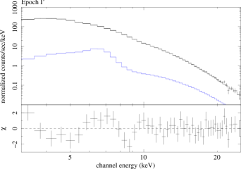
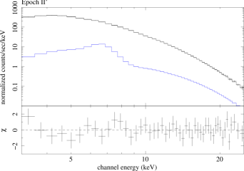
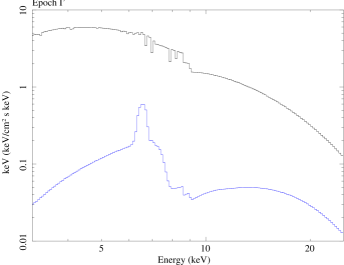
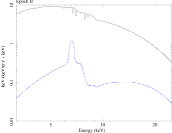
Figure 7.— Upper: The RXTE PCA spectra (with error bars) folded with the energy response in Epoch I’ (left) and II’ (right). The upper curve (black) represents the best-fit model including the contribution of the reflection component (lower curve, blue). The lower panel shows the residuals of the data from the best-fit model, normalized by the error (i.e., in units of $\chi$). Lower: the best-fit model in the form of $E^{2}F_{E}$, where $E$ and $F_{E}$ is the energy and photon spectrum, respectively, in Epoch I’ (left) and Epoch II” (right). The lower curve (blue) represents the reflection component.

Table 4Best-Fit Parameters of the RXTE PCA Spectra

Parameter	Unit		Epoch I’	Epoch II’
$r_{\rm in}$	(km)		113$\pm$7	79$\pm$8
$T_{\rm in}$	(keV)		0.87$\pm$0.06	1.11$\pm$0.06
$T_{\rm e}$	(keV)		3.62${}^{+0.52}_{-0.24}$	3.66${}^{+0.34}_{-0.25}$
$\Gamma$			3.18${}^{+0.17}_{-0.15}$	2.99$\pm$0.14
( $\tau_{\rm e}$			4.8$\pm$0.3	5.2$\pm$0.4 )
$\Omega_{\rm refl}/2\pi$			0.5${}^{+0.0}_{-0.06}$	0.42${}^{+0.08}_{-0.19}$
$\xi_{\rm refl}$	(erg cm s-1)		20 (fixed)	40 (fixed)
$\tau_{\rm edge}$ (9.0 keV)			0.25$\pm 0.02$	0.16$\pm$0.03
$\tau_{\rm edge}$ (8.6 keV)			0.28$\pm 0.03$	0.07$\pm$0.02
$F_{2-10}$	(erg cm-2 s-1)		$1.0\times 10^{-8}$	$1.6\times 10^{-8}$
$L_{0.01-100}$	(erg s-1)		$6.6\times 10^{38}$	$8.3\times 10^{38}$
$\chi^{2}$ (d.o.f)			40.4 (43)	24.1 (43)

Note. — The errors are 90% confidence level for a single parameter.

4. Discussion

4.1. Nature of Accretion Disk Wind

We have detected at least 32 narrow absorption lines from a highly ionized plasma (H-like or He-like) in the HETGS spectra of GRS 1915+105 in “soft state” that are the deepest among those detected from the source, achieving our primary aim with this ToO observation. This enables us to investigate the physical properties of the plasma with the best accuracy ever achieved. The velocity and line-of-sight velocity dispersion are determined to be 150–500 km s^-1 and 70–200 km s^-1, respectively, which differ by element. Since the proper motion of GRS 1915+105 is estimated at $3\pm 10$ km s^-1 from Greiner, Cuby, & McGaughrean (2001) (considering the fact that the black hole mass is about 12 times larger than the companion in this system), it is revealed that the plasma is definitely in outflow, and hence the origin is a wind (most likely an accretion disk wind) as suggested in previous studies (Lee et al., 2002). The depth of these absorption lines changed according to the X-ray flux, consistent with the picture that it is photo-ionized by the radiation.

Estimating the location of the wind is crucial to discriminate its origin. We estimate it by a simple argument using the ionization parameter $\xi=L/nr^{2}$ (Tarter et al., 1969), where $L$ is the luminosity, $n$ is the density, and $r$ is the distance from the source. As discussed below, $\xi$ may not always constant along the line of sight but here we discuss its averaged value for first order estimate. For this purpose, we perform simulation of a photoionized plasma by the XSTAR code for various values of $\xi$, assuming our best-fit continuum models in Table 4 and the metal abundances in Table 1. The density $n$ is set to be $10^{12}$ cm^-3. We find that the observed number ratio between Fe XXVI and Fe XXV ions, 1.8$\pm$1.0 and 4.5$\pm$1.5, indicates log $\xi=4.3^{+0.1}_{-0.6}$ and log $\xi=4.2\pm 0.1$ for Epoch I and II, respectively; here $L$ is defined in the 0.0136–13.6 keV band in each spectrum (this is the reason why the $\xi$ value is larger in Epoch I in spite of the lower ionization state). Assuming that the length of the wind, $\Delta r$, is a similar order to the distance from the source, we find $nr\sim n\Delta r\sim 10^{23}$ cm^-2 after correcting for the fraction of Fe XXVII ions and Fe abundance of 3.6 times the solar. This yields $r\sim L/\xi/nr\sim(2-6)\times 10^{11}$ cm, or $\sim(1-3)\times 10^{5}\;r_{\rm g}$ for a black hole mass of 14 ${\rm M_{\odot}}$. This well exceeds a possible minimum launching point of thermally driven wind from an X-ray irradiated disk theoretically predicted. The critical radius where the thermal energy of the X-ray heated disk exceeds the gravitational energy is given by

$$r_{\rm c}\sim 10^{10}(\frac{10^{8}\;{\rm K}}{T_{\rm C}})(\frac{M}{\mbox{${\rm M_{\odot}}$}})\;\;{\rm cm}.$$

Here $T_{\rm C}$ is the Compton temperature, at which the net energy transfer between electrons and photons is balanced out. In our case $T_{\rm C}$ is estimated to be $\sim$0.3 keV by taking the average of photon energy of the continuum in the 0.01–100 keV band, and hence $r_{\rm c}\sim 4\times 10^{12}$ cm. It is predicted that such wind can be launched from $\sim 0.1r_{\rm c}$ or even much smaller radii (Woods et al., 1996). As the luminosity ($>6.6\times 10^{38}$ erg s^-1 in the 0.1–100 keV band) is about 0.3 times the Eddington limit, the effect of radiation should be also important even if the gas is highly ionized and the opacity by UV-lines is little. Thus, the wind we observe is consistent with a thermally (plus radiation) driven wind and there is no necessity to invoke a magnetically driven wind.

The mass outflow rate carried by the accretion disk wind is evaluated as

$$\dot{M}_{\rm out} = \Omega_{\rm wind}r^{2}nm_{\rm p}v_{\rm wind}$$

$$\sim (0.6-1.3)\times 10^{19}\;(\frac{\Omega_{\rm wind}/4\pi}{0.2})(\frac{v_{\rm wind}}{500\;{\rm km\;s^{-1}}})\;\;{\rm g\;s^{-1}}.$$

Here we have used $r^{2}n=L/\xi\sim(3-6)\times 10^{34}$, $m_{\rm p}$ is the proton mass, $\Omega_{\rm wind}$ is the solid angle of the wind, and $v_{\rm wind}$ is the outflow velocity (which is larger than the observed outflow velocity by a factor of cosine of the angle between the direction of the wind and our line-of-sight). Thus, the mass outflow rate carried by the wind could be comparable to the mass accretion rate in the inner part of the disk, which is estimated to be $(0.7-0.9)\times 10^{19}$ g s^-1 (spherical case) or $(2-3)\times 10^{19}$ g s^-1 (disk-like case) by assuming the mass-to-energy conversion efficiency of 0.1. This demonstrates the importance of the wind for understanding the dynamics of the whole disk system. A similar situation is found in the neutron star low mass X-ray binary GX 13+1 (Ueda et al., 2004) except for the difference of the mass scale.

We find that H-like ions of heavier elements have higher outflow velocity and larger velocity dispersion. In addition, there is an implication that Fe XXV shows a smaller velocity than that of Fe XXVI, although we have to keep in mind the possible systematic uncertainties in the obtained parameters for Fe XXV. These results indicate that we trace different parts of the wind by different ions; there is a component of the flow that is more highly ionized (i.e., traced by Fe XXVI) and that is moving approximately 3 times faster than the gas traced by other lines. According to a thermally driven wind model (see Netzer, 2006, and references therein), the velocity of outflow can be represented in a power law form of distance,

$$v\propto r^{\gamma},$$

where $\gamma$ is in the range of 0–0.5. Then, from the conservation of the mass outflow rate, the density is given as

$$n\propto r^{-2-\gamma},$$

and therefore

$$\xi\propto r^{\gamma}.$$

For $\gamma>0$, ionization becomes stronger at outer parts of the wind. In this interpretation, H-like Si ions we observe must be located closer to the center where $\xi$ is smaller, and hence have a smaller outflow velocity, compared with those of H-like Fe ions. The larger velocity dispersion found in heavier element of H-like ions can be attributed to a larger line-of-sight velocity gradient when integrated in a more outer region of the wind, probably accompanied by larger turbulent motion as well. Constructing a fully quantitative model for the wind of GRS 1915+105 is beyond the scope of this paper and is left for future studies.

4.2. Origin of X-ray Continuum Emission in “Soft State”

The ideal combination of the Chandra HETGS and RXTE PCA has enabled us to constrain the continuum model with least uncertainties, by correctly taking into account the interstellar absorption with the (updated) anomalous abundances and local spectral features including absorption- and emission lines. The spectra of GRS 1915+105 in “soft state” (steady State A in the definition of Belloni et al. 2000) in the 1–25 keV band can be well explained with a strongly Comptonized continuum and its reflection component by an outer part of the disk, which is absorbed by a highly ionized disk wind discussed above.

A relativistically broadened iron-K emission line as previously reported by Martocchia et al. (2002) is not required in our data, although it is difficult to perfectly exclude its presence from the spectral fit alone, which strongly depends on the continuum model (and also on the interstellar absorption). The large inner radius we obtained from the line profile with the Chandra HETGS, $400r_{\rm g}$, does not necessarily mean that the accretion disk is truncated at that radii. Rather, as discussed below, due to the strong Comptonization by corona that completely covers the inner disk, any iron-K features arising there should be smeared out. This makes extremely difficult to constrain the innermost radius of the accretion disk from the iron-K emission profile.

We find that a thermal Comptonization is the most likely origin of the continuum emission of GRS 1915+105 in “soft state”. The standard, MCD plus a power law description for the continuum does not give acceptable fit. Instead of the MCD model, the $p$-free disk model, expected from a one-dimensional slim disk (Abramowicz et al., 1988), gives a statistically acceptable fit to the spectrum in Epoch II’. We consider it physically unlikely, however, because the inferred innermost radius is too small ($\lower 2.15277pt\hbox{$\;\buildrel<\over{\sim}\;$}0.3r_{\rm g}$) than a theoretical prediction (Watatai et al., 2000). Also, we cannot consistently explain the spectra of two epochs with the same model.

The spectral model of Comptonization yields an optical depth $\approx 5$ and a low electron temperature ($\approx$4 keV) for either of the two brightness levels that were sampled with the PCA. The seed photon spectrum is consistent with the emission from a standard disk (MCD). No direct disk component is required from the fit. In this interpretation, most of the radiation energy is produced in the Comptonization corona, which completely covers the inner part of the disk. Our results basically support the conclusion by Done et al. (2004), who analyzed 7 representative PCA spectra of GRS 1915+105 in various states and found that thermal Comptonization is a dominant spectral component in most (5 out of 7) cases. In their color-color diagram (see their Figure 4), our spectra are located at the positions of $(1.23,0.45)$ and $(1.45,0.52)$, which are closest to obs. 7 and 6 for Epochs I’ and II’, respectively. Done et al. (2004) favor a MCD-dominant model for both obs. 7 and 6 rather than a purely Comptonized spectrum, however. The reason for this discrepancy is unclear.

In the Comptonization model, we can infer the innermost radius ($r_{\rm in}$) of the accretion disk injecting the seed photons to the corona, by the conservation of photon number in the Comptonization process. For this purpose, we adopt the formula (A1) of Kubota & Makishima (2004) with the left-hand term increased by a factor of two,

$$2\;F_{\rm thc}^{p}\;2{\rm cos}(i)=0.0165\;[\frac{r_{\rm in}^{2}\;{\rm cos}(i)}{(D/10\;{\rm kpc})^{2}}]\;(\frac{T_{\rm in}}{1\;{\rm keV}})^{3}\;\;{\rm photons\;s^{-1}\;cm^{-2}},$$

where $F_{\rm thc}^{p}$ is 0.01–100 keV photon flux from the Comptonized component. Here we have assumed that half of photons in the corona is injected again into the accretion disk due to the large optical depth ($\approx 5$). The results are given in Table 4. For isotropic emission of the Comptonized component, we find $r_{\rm in}$ $\approx$110 km and $\approx$80 km for Epoch I’ and II’, respectively (instead, if the optically thick corona has a thin disk-like geometry, the $2{\rm cos}(i)$ factor in the left term must be ignored and hence $r_{\rm in}$ is increased by about 20%). The estimated $r_{\rm in}$ values correspond to $\approx 5r_{\rm g}$ (Epoch I’) and $\approx 4r_{\rm g}$ (Epoch II’). With correction for the color-to-effective temperature and that for the inner boundary condition (see Kubota et al., 1998), the physical radius would be larger than these values by a factor of 1.2. Thus, based on the innermost temperature and photon numbers, the optically-thick disk may extend down only to $\lower 2.15277pt\hbox{$\;\buildrel>\over{\sim}\;$}4r_{\rm g}$ in this state, not to the innermost stable circular orbit (ISCO) of $1.23r_{\rm g}$ for a maximally rotating Kerr hole. If the radius observed in Epoch II’ indeed corresponds to the ISCO, then our result indicates that the black hole spin of GRS 1915+105 is only moderate, supporting the conclusion by Middleton et al. (2006).

Of all the classes of light curves for GRS 1915+105, the $\phi$ class signifies conditions when the source is most soft and steady. In most BHBs, these conditions are associated with the high/soft state, in which a MCD component dominates the X-ray spectrum while there are low levels of Comptonization (Remillard & McClintock, 2006), normally observed at lower fractions of the Eddington rate than in our case (0.3–1.2 $L/L_{\rm Edd}$ depending on the geometry of the emitting region). Our analyses show that this is not the case for our $\phi$ state observations of GRS 1915+105, where Comptonization dominates. Furthermore, the 67 Hz X-ray QPO can be considered as additional signs of disturbances that lead away from the simple MCD that we envision for the high/soft state. Such disturbances are chronic properties of GRS 1915+105 in its soft states. McClintock et al. (2006) were able to find only 20 high/soft state examples in an archive of $\sim 1000$ RXTE pointings that included $\sim 150$ observations of soft and steady conditions (classes $\phi$, $\delta$, and some $\gamma$ types).

Such strongly Comptonized spectra are characteristics of the very high state (VHS) of other BHBs observed at luminosities of $\sim 0.5L/L_{\rm Edd}$ (e.g., Kubota & Makishima, 2004), although the electron temperature of the Comptonizing corona in the VHS is much higher ($>10$ keV) than our case ($\approx$4 keV). This suggests that the “soft state” of GRS 1915+105 corresponds to the VHS of canonical BHBs, but the electrons in the corona must be more efficiently cooled by Comptonization. It could be explained because the disk extends to small radii in the “soft state” of GRS 1915+105, hence providing many soft photons to the corona, while the disk of other BHBs in the VHS may be truncated at larger radii (Kubota & Done 2004; see also Done & Kubota 2006). To confirm this picture, more systematic studies of GRS 1915+105 in similar states at different luminosities are important.

There is a puzzling combination of a fast QPO and spectral indications of strong Comptonization, and this has been seen in other sources as well (Remillard & McClintock, 2006). If the oscillations originate in the disk, then the Comptonizing corona must be sufficiently compact to avoid suppression of the 67 Hz oscillations due to scattering effects; for $\tau_{\rm e}$=5 the size must be much smaller than $\sim 10r_{\rm g}$. Alternatively, the formation of the corona may involve asymmetries or waves related to energy injection mechanisms. There is insufficient data to determine if all of the soft-state properties of GRS 1915+105 that deviate from the high/soft state appear to be correlated. However, such knowledge would assist efforts to understand the cause of Comptonization and the mechanisms and interpretive values of the QPO frequencies.

References

- Abramowicz et al. (1988) Abramowicz, M.A., Czerny, B., Lasota, J.P., Szuszkiewicz, E. 1998, ApJ, 332, 646
- Anders & Grevesse (1989) Anders, E. & Grevesse, N. 1989, Geochimica et Cosmochimica Acta, 53, 197
- Arai et al. (2008) Arai, A. et al. 2008, submitted to PASJ
- Begelman et al. (1983) Begelman, M.C., McKee, C.F., Shields, G.A. 1983, ApJ, 271, 70
- Belloni et al. (2000) Belloni, T., Klein-Wolt, M., Mendez, M., van der Klis, M., & van Paradijs, J., 2000, A&A, 355, 271
- Boirin et al. (2004) Boirin, L., Parmar, A.N., Barret, D., Paltani, S., Grindlay, J.E. 2004, A&A, 418, 1061
- Done & Kubota (2006) Done, C. & Kubota, A. 2006, MNRAS, 371, 1216
- Done et al. (2004) Done, C., Wardziński, G., & Gierliński, M. 2004, MNRAS, 349, 393
- Draine (2003) Draine, B.T. 2003, ApJ, 598, 1026
- Fender & Belloni (2004) Fender, R. & Belloni, T. 2004, ARA&A, 42, 317
- Girlinski et al. (1997) Girlinski, M. et al. 1997, MNRAS, 288, 958
- Greiner, Cuby, & McGaughrean (2001) Greiner, J., Cuby, J.G., & McCaughrean, M.J., 2001, Nature, 414, 522
- Kubota et al. (1998) Kubota, A., Tanaka, Y., Makishima, K., Ueda, Y., Dotani, T., Inoue, H., Yamaoka, K. 1998, PASJ, 50, 667
- Kubota & Makishima (2004) Kubota, A. & Makishima, K. 2004, ApJ, 601, 428
- Kubota & Done (2004) Kubota, A. & Done, C. 2004, MNRAS, 353, 980
- Fabian et al. (1989) Fabian, A.C., Rees, M.J., Stella, L., White, N.E. 1989, MNRAS, 238, 729
- Jahoda et al. (2006) Jahoda, K., Markwardt, C.B., Radeva, Y., Rots, A.H., Stark, M.J., Swank, J.H., Strohmayer, T. E., & Zhang, W. 2006, ApJS, 163, 401
- Kotani et al. (2000) Kotani, T., Ebisawa, K., Dotani, T., Inoue, H., Nagase, F., Tanaka, Y., Ueda, Y. 2000, ApJ, 539, 413
- Lee et al. (2002) Lee, J.C., Reynolds, C.S., Remillard, R., Schulz, N.S., Blackman, E.G., Fabian, A.C. 2002, ApJ, 567, 1102
- Magdziarz & Zdziarski (1995) Magdziarz, P. & Zdziarski, A. A. 1995, MNRAS, 273, 837
- Makishima et al. (2008) Makishima, K. et al. 2008, PASJ, 60S, 585
- Martocchia et al. (2002) Martocchia, A., Matt, G., Karas, V., Belloni, T., Feroci, M. 2002, A&A, 387, 215
- Masai & Ishida (2004) Masai, K., & Ishida, M. 2004, ApJ, 607, 76
- McClintock et al. (2006) McClintock, J. E., Shafee, R., Narayan, R., Remillard, R. A., Davis, S. W., & Li, L.-X. 2006, ApJ, 652, 518
- Middleton et al. (2006) Middleton, M., Done, C., Gierliński, M. Davis, S.W. 2006, MNRAS, 373, 1004
- Miller et al. (2006) Miller, J. M. et al. 2006, Nature, 441, 953
- Mineshige et al. (1994) Mineshige, S., Hirano, A., Kitamoto, S., Yamada, T.T., Fukue, J. 1994, ApJ, 426, 308
- Mitsuda et al. (1984) Mitsuda, K., et al. 1984, PASJ, 36, 741
- Morgan, Remillard, & Greiner (1997) Morgan, E.H., Remillard, R.A., & Greiner, J., 1997, ApJ, 482, 993
- Netzer (2006) Netzer, H. 2006, ApJ, 652, 117
- Proga, Stone, & Kallman (2000) Proga, D., Stone, J.M., Kallman, T.R. 2000, ApJ, 543, 686
- Remillard & McClintock (2006) Remillard, R. A. & McClintock, J. E. 2006, ARA&A, 44, 49
- Rothschild et al. (1998) Rothschild, R.E. et al. 1998, ApJ 496, 538
- Sunyaev & Titarchuk (1980) Sunyaev, R.A. & Titarchuk, L.G. 1980, A&A, 86, 121
- Takahashi et al. (2008) Takahashi, H. et al. 2008, PASJ, 60S, 69
- Tanaka & Lewin (1995) Tanaka, Y., & Lewin, W.H.G. 1995, in X-Ray Binaries, ed. W.H.G. Lewin, J. van Paradijs, & E.P.J. van den Heuvel (Cambridge: Cambridge Univ. Press), 126
- Tarter et al. (1969) Tarter, C.B., Tucker, W., Salpeter, E.E. 1969, ApJ, 156, 943
- Toor & Seward (1974) Toor, A. & Seward, F.D., 1974, AJ, 79, 995
- Ueda et al. (1998) Ueda, Y., Inoue, H., Tanaka, Y., Ebisawa, K., Nagase, F., Kotani, T., Gehrels, N. 1998, ApJ, 492, 782; 1998, ApJ, 500, 1069 (Erratum)
- Ueda et al. (2001) Ueda, Y., Asai, K., Yamaoka, K., Dotani, T., Inoue, H. 2001, ApJ, 556, L87
- Ueda et al. (2004) Ueda, Y., Murakami, H., Yamaoka, K., Dotani, T., Ebisawa, K. 2004, ApJ, 609, 325
- Ueda et al. (2005) Ueda, Y., Mitsuda, K., Murakami, H., Matsushita, K. 2005, ApJ, 620, 274
- Watatai et al. (2000) Watarai, K., Fukue, J., Takeuchi, M., Mineshige, S. 2000, PASJ, 52, 133
- Wilms et al. (2000) Wilms, J, Allen, A., McCray, R. 2000, ApJ, 542, 914
- Woods et al. (1996) Woods, D.T., Klein, R. I., Castor, J.I., McKee, C.F., Bell, J.B. 1996, ApJ, 461, 767
- Zhang et al. (1995) Zhang, W., Jahoda, K., Swank, J.H., Morgan, E,H, Giles A.B., 1995, ApJ, 449, 930
- Życki, Done, & Smith (1999) Życki, P. T., Done, C., Smith, D.A. 1999, MNRAS, 309, 561