“Old” Locked Inflation

Abstract

In this paper, we revisit the idea of locked inflation, which does not require a potential satisfying the normal slow-roll condition, but suffers from the problems associated with “saddle inflation”. We propose a scenario based on locked inflation, however, with an alternative evolution mechanism of the “waterfall field” $\phi$. Instead of rolling down along the potential, the $\phi$ field will tunnel to end the inflation stage like in old inflation, by which the saddle inflation could be avoided. Further, we study a cascade of old locked inflation, which can be motivated by the string landscape. Our model is based on the consideration of making locked inflation feasible so as to give a working model without slow roll; It also can be seen as an effort to embed the old inflation in string landscape.

1 Introduction

Recently, substantial efforts have been invested in understanding how to embed inflationary models in supergravity and the string landscape, e.g.[1, 2, 3]. However, since the moduli fields which is naively expected to be natural candidate of inflaton fields generally have protected masses $m\sim H$, and the required slow roll condition $\eta\sim m^{2}/H^{2}\ll 1$, ($m$ is the mass of the field and $H$ the Hubble parameter during inflation) is violated. This $\eta$-problem is encountered in attempts to embed inflation in the string landscape. Recently, Dvali and Kachru [4, 5] have proposed locked inflation. It is slightly similar to hybrid inflation[6], but here the slow roll constraint is not required. In locked inflation, the oscillations of a scalar field will trap the “waterfall field” at the top of its saddle point for a period. The potential energy at the saddle then drives inflation. This model, if consistent, overcomes the hurdles faced by slow roll inflation in supergravity and string theories. Without the extremely flat potential, density perturbations cannot be created by the same mechanism as in ordinary inflationary models. A suggestion[7, 8] of alternative mechanism to generate density perturbation was adopted.

However, Easther et al. analyzed the cosmological consequences of locked inflation[9]. Their work showed that a period of saddle inflation is possible to follow the locked inflationary era, which will lead to some problems. To avoid this disastrous outcome associated with saddle inflation, strong constraints on the parameter space open to models of locked inflation must be put. Afterwards, Copeland and Rajantie extended the investigation for locked inflation[10]. They considered many constraints arising from density perturbations, loop corrections, parametric resonance and defect formation, and found that it is impossible to satisfy all of these constraints without having a period of saddle inflation afterwards. Their conclusion was quite strong, and it seemed “the end of locked inflation”.

We, in this paper, propose an inflation scenario, which inherits the merit of locked inflation while avoids its fatal problems. This scenario has the same dynamics of the oscillating field but an alternative mechanism of the evolution of the “waterfall field”. Instead of rolling down along the potential, the “waterfall field” will tunnel to end the inflation stage as in old inflation[11]. In our model, we need a cross-coupling $\frac{1}{2}\lambda\phi^{2}\Phi^{2}$ term in the potential as well. But instead of at saddle point, inflation takes place when a scalar field keeps oscillating at the bottom of a local minimum, which means at $\Phi=0$ the “waterfall field” $\phi$ has a positive rather than negative mass-squared. This feature is more natural in certain multi-field inflationary setups within stringy landscape, where each local minimum is relative with a cosmological constant respectively. We assume that this barrier is easy for rapid tunneling. However, due to the existence of the coupling constant, the non-zero vacuum expectation value of the oscillating $\Phi$ field produces an additional mass term $\frac{1}{2}\lambda\langle\Phi^{2}\rangle$ for $\phi$, which makes the barrier that along the direction of $\phi$ enhanced. This is helpful to trap the field in the false vacuum for a period, thereby a large e-foldings could be provided. As time goes by, the reduction of the $\Phi$ amplitude lead to the attenuation of the barrier of $\phi$, which causes $\phi$ tunneling. In this way we could overcome the shortcoming of original locked inflation.

In section II, we start with the basic points of the locked inflation model, and then illustrate the constraints or failure of it. In section III, first we take a look at the relationship between barrier and the tunneling probability, as well as the idea of time dependent decay rate. Then, we present our inflation scenario. We will expand our scenario and give a generalization in section IV. In the appendix we present a concrete example to illustrate our general ideas and analyze the time dependence of the expansion rate. Our conclusions are summarized in section V.

2 Locked Inflation

Consider two scalar fields $\Phi$ and $\phi$ with a potential the same form as normal hybrid inflation [6], but notice that here at nopoint dose this potential satisfy the standard slow-roll requirements

$$V(\Phi,\phi)=\frac{1}{2}m_{\Phi}^{2}\Phi^{2}+\frac{1}{2}\lambda\Phi^{2}\phi^{2}+\frac{\alpha}{4}\left(\phi^{2}-M_{*}^{2}\right)^{2},$$ (1)

where $\lambda$ is a dimensionless free parameter. At $\Phi=\phi=0$, the “waterfall field” $\phi$ has a negative mass-squared $-\alpha M_{*}^{2}$.

Generally, the necessity of slow roll lies in that it guarantees the model a sufficient e-foldings and give a scale invariant spectrum which is required by the observation. The usual slow-roll parameter $\eta_{\Phi}$, is given by

$$\eta_{\Phi}=M_{P}^{2}\frac{V^{\prime\prime}}{V}=\frac{m_{\Phi}^{2}}{3H^{2}},$$ (2)

where $M_{P}=(8\pi G)^{-1/2}$ is the reduced Planck mass. Slow roll inflation requires $\eta_{\Phi}\ll 1$, but here $m$ is of order $H$. So $\Phi$ rolls toward its stationary point with certain speed, but overshoots and performs oscillations near the origin which lock the $\phi$ field in its instability region. At the beginning the oscillation energy might be comparable to the false vacuum energy, but it gets redshifted and the energy density will be dominated by the latter

$$V=V(0,0)=\frac{\alpha}{4}M_{*}^{4}.$$ (3)

This leads to an inflationary phase with an expansion rate

$$H^{2}\approx\frac{V}{3M_{P}^{2}}=\frac{m_{\phi}^{2}M_{*}^{2}}{12M_{P}^{2}}.$$ (4)

The redshift causes the oscillating $\Phi$ field a decreasing amplitude

$$(\frac{\Phi_{A}(t)}{\Phi_{initial}})^{2}\sim(\frac{a_{initial}}{a(t)})^{3}.$$ (5)

That is

$$\Phi_{A}(t)=\Phi_{initial}\ e^{-\frac{3}{2}Ht}.$$ (6)

Eventually, these oscillations are sufficiently damped to allow the field point to roll off the saddle point in the $\phi$ direction, thereby ending locked inflation. The critical amplitude $\Phi_{C}$ is the value of the amplitude when the effective mass of $\phi$

$$m_{eff}^{2}\simeq\lambda\Phi_{A}(t)^{2}-\alpha M_{*}^{2}$$ (7)

is reduced to zero, which means $\Phi_{C}=\sqrt{\alpha/\lambda}M_{*}$. This implies that the number of e-foldings is

$$N\simeq\frac{2}{3}\ln\frac{\Phi_{initial}}{\Phi_{C}}\approx\frac{1}{3}\ln\frac{\lambda\Phi_{initial}^{2}}{m_{\phi}^{2}}.$$ (8)

By plugging in some representative numbers ($M_{*}\sim M_{P},M\sim Tev,\lambda\sim 1$, and $\Phi_{initial}\sim M_{P}$), they get $N\simeq 50$ or so. This allows the bubble to grow sufficiently large to contain our present horizon volume.

The key point of this model is that the dynamics of the first field keep the second field trapped in a false minimum, resulting in an evanescent period of inflation. However, firstly, the oscillation maybe spoiled. We can tell from the equation of $\Phi$ that there is an additional constraint on $m_{\Phi}$. If it is too small($<3H/2$), $\Phi$ will be overdamped, and no oscillation will occur. If $m_{\Phi}$ is too large ($>10H$), one can produce $\Phi$ particles via parametric resonance, and the kinetic energy will be drained from the $\Phi$ field rapidly, undermining locked inflation[9]. Secondly, Easther et al. also pointed out that there should be a period of “saddle inflation”, which results in a strongly scale dependent spectrum that is inconsistent with observation even lead to massive black hole formation in the primordial universe right after the locked inflation, even if the usual slow-roll parameter $\eta_{\phi}=m_{\phi}^{2}/3H^{2}$ is greater than unity.

For multiple scaler field, $\textit{P}_{\xi}=(\frac{H}{2\pi})^{2}\sum(\frac{\partial N}{\partial\phi^{\textit{i}}})^{2}$. As will be argued in §3.2, at the saddle point, where the rate of the slope is small, a slight change in the field value along the “waterfallfield” direction can cause a big variation of the e-foldings, leading to a large $\frac{\partial N}{\partial\phi}$, and also it is the fact that there are two down hill directions rather than one, leading to further amplifications. Hence modes leave the horizon at the onset of saddle inflation will cause massive black hole formation when they reenter the horizon. One way out of this black hole problem is to let the saddle inflation era last long enough to move this troublesome modes outside of the present cosmological horizon, as well as all the signatures of the locked inflation. However, this long period of saddle inflation needs $\eta\ll 1$, to find a way to avoid which is exactly our work’s motivation. Further, the existence of the long saddle inflation might cause the locked inflation unphysical from the viewpoint of the Trans-Planckian Problem. Hence, to make the locked inflation feasible, one must find a method to avoid bringing about saddle inflation or black hole[12]. Further, Copeland and Rajantie[10] considered various constraints arising from density perturbations, loop corrections, parametric resonance and defect formation. In their results, the most salient and unnatural feature is that the value of parameter $\eta_{\phi}$ is supposed to be very large. First, they figured out that to avoid saddle inflation, the value of $\eta_{\phi}$ has to be no less than $10^{3}$; Second, the defect formation will impose a constraint on $\eta_{\phi}$ with $\eta_{\phi}\gtrsim 10^{6}$. In addition, loop correction leads to $\eta_{\Phi}\mathop{\raise 1.29167pt\hbox{$>$\kern-7.5pt\raise-4.73611pt\hbox{$\sim$}}}\eta_{\phi}/2$, and the condition with parametric resonance would stop inflation during the first e-folding unless $\eta_{\Phi}\mathop{\raise 1.29167pt\hbox{$<$\kern-7.5pt\raise-4.73611pt\hbox{$\sim$}}}70$. The whole parameter space available for locked inflation is ruled out, especially that constraints on $\eta_{\phi}$ is too strong and it’s unnatural thus can’t be satisfied. It is also clear that if saddle inflation can be avoided by some mechanism, leaving the requirements of parametric resonance and loop corrections, locked inflation would be feasible. And the demand of moduli fields in supergravity and string theory ($\eta\geq{\cal O}(1)$) would also be met.

3 “Old” Locked Inflation

3.1 Time-Dependent Nucleation Rate

Coleman et al. developed the qualitative and quantitative semiclassical theory of the decay of a false vacuum[13, 14, 15]. The vacuum of higher energy density is a stable classical equilibrium state. However, it is rendered unstable by quantum effects by barrier penetration, which produces bubbles of true vacuum in the sea of false vacuum. We are talking about the formation of the bubble, and this process takes place on scales at which gravitational effects are negligible. It is possible to obtain explicit expressions in the limit of small $\epsilon$, the energy density difference between the two vacua. The decay rate per unit volume $\Gamma$ associated with this process is given by an expression of the form[14, 16] $\Gamma\sim e^{-B}$, and the coefficient $B$ is the total Euclidean action for the bounce

$$B={27\pi^{2}S_{1}^{4}\over 2\epsilon^{3}},$$ (9)

where $S_{1}=\int\sqrt{2V}\mathrm{d}\phi$ depends on the height, width and shape of the barrier.

Because $\Gamma$ is the exponential function of $B$, the decay rate of the false vacuum is extremely sensitive to the parameters of the potential. As the tunneling rate is so sensitive to $S_{1}$and $\epsilon$, the transition from a long-living field to a rapid tunneling field requires only a small change of the potential. This could be realized by a little reduction of the height or width of the barrier as well as sort of enhancement of the initial and final energy difference $\epsilon$.

The lifetime of the false vacuum is about $\tau=\frac{3}{4\pi}\frac{H^{3}}{\Gamma}$[17, 18]. The dimensionless quantity $\frac{\Gamma}{H^{4}}$ is the volume fraction of space occupied by bubbles nucleated over a hubble time. Old inflation required $\frac{\Gamma}{H^{4}}\ll 1$, so that enough e-foldings could be provided, but the production of bubbles of true vacuum is rare which means bubbles could not collide with each other and thermalization could not be achieved. And to successfully end the inflation a general condition, $\frac{\Gamma}{H^{4}}\geq 9/4\pi$, must be satisfied[17, 18]. People realized that to solve the problem one needed a time dependent nucleation rate for a single tunneling field, i.e. $\frac{\Gamma}{H^{4}}$ started out small so that the universe inflated and later due to some mechanism, $\frac{\Gamma}{H^{4}}$ for the tunneling field became large so that the phase transition suddenly took place and completely throughout the universe.

The variation of both $\Gamma$ and $H$ is frame dependent. In extended [19] and hyperextended[20, 21] inflation, the Hubble constant becomes time-dependent due to Brans-Dicke gravity[22]. Later, approaches to obtain a time-dependent decay rate utilizing two coupled scalar fields were proposed[23, 24, 25]. Adams and Freese found that in order to bring about sufficient e-foldings the potential of the employed rolling field must be flat just as in slow roll condition. In this paper we go further down this route, proposing a landscape-based model without slow-roll.

3.2 “Old” Locked Inflation

In section II, we mentioned that if saddle inflation could be avoided by some mechanism, locked inflation would be feasible, and the feature of moduli fields in supergravity and string theory ($\eta\geq{\cal O}(1)$) would also be met. We find out a different evolution of the $\phi$ field so as to turn the saddle inflation era away. By achieving this, the failure of locked inflation talked in section II could be circumvented.

We will introduce the same dynamics of the oscillating field but an alternative mechanism of the evolution of the “waterfall field”. Instead of at saddle point, inflation takes place when a scalar field keeps oscillating at a bottom of a local minimum, which means at $\Phi=0$ the “waterfall field” $\phi$ has a positive other than negative mass-squared. We assume that this barrier is easy for rapid tunneling. However, due to the existence of the coupling constant, the non-zero vacuum expectation value of the oscillating $\Phi$ field produces an additional mass term $\frac{1}{2}\lambda\langle\Phi^{2}\rangle$ for $\phi$, which makes the barrier that along direction of $\phi$ enhanced. This is helpful to trap the field in the false vacuum for a period, thereby a large e-foldings could be provided. As time goes by, the reduction of the $\Phi$ amplitude lead to the attenuation of the barrier of $\phi$, which causes $\phi$ tunneling. In this sense, this scenario is slightly similar to old inflation, thus called “old” locked inflation.

There are several benefits in our model. First, it would be more natural to assume local minima, if the scenario is based on string landscape. Second, saddle Inflation is avoided, thus the merit of locked inflation can be reserved and the parameter space available is nice. Third, it would be more general as it includes both rolling and tunneling, however, we don’t need the potential to satisfy the slow-roll conditions at all.

As the value of $\frac{\Gamma}{H^{4}}$ is extremely sensitive to the parameter in the potential, a little modification of the barrier could lead to a transition from slow to rapid tunneling. Due to the existence of the coupling term, the barrier would be higher where the value of $|\Phi|$ is larger, thus tunneling would be more rare. As a result, there would be an area inside which $\frac{\Gamma}{H^{4}}\sim{\cal O}(1)$ and outside $\frac{\Gamma}{H^{4}}\ll{\cal O}(1)$ (see a visual illustration in Fig.3 in A).

The value of $|\Phi|$ at this edge is denoted as $\Phi_{ep}$, meaning $\phi$ is easy to be penetrated when $|\Phi|$ is less than this value. Tunneling happens when the time that the field point takes to move inside the easy tunneling region ($|\Phi|\leq\Phi_{ep}$) is longer than the vacuum lifetime $\tau$. In the process of oscillation, potential energy of $\Phi$ ($V_{\Phi}=\frac{1}{2}m_{\Phi}^{2}\Phi_{amplitude}^{2}$) is translated into kinetic energy at the lowest point with a velocity of $m_{\Phi}\Phi_{amplitude}$. So the time $\Phi$ spends in the easy-tunneling region is approximately

$$\Delta t\simeq\frac{2\Phi_{ep}}{m_{\Phi}\Phi_{amplitude}}$$ (10)

And in this region, the time that penetrating takes is approximately

$$\tau=\frac{3}{4\pi}\frac{H^{3}}{\Gamma}.$$ (11)

So, the critical amplitude of the end of the inflationary phase $\Phi_{crit}$ is

$$\Phi_{crit}=\frac{2\Phi_{ep}}{m_{\Phi}\tau}=\frac{8\pi\Phi_{ep}}{3m_{\Phi}}\frac{\Gamma}{H^{3}}$$ (12)

There is no definite results of the calculation of the vacuum decay rate yet. To give some rough numerical values, we need to give the initial and critical value of $\phi$. Nevertheless, the choice of the critical value $T_{ep}$ (around where $\frac{\Gamma}{H^{4}}$ jumps from $\ll 1$ to $\geq 9/4\pi$) has great liberty, since the parameters of the least resistance barrier is not determined. Considering that $\Phi_{ep}$ is reasonable to be at the value where the effective mass of $\phi$ arising from the coupling term $\lambda\Phi^{2}$ is on the same scale of mass term $m_{\phi}^{2}$,

$$\lambda\Phi_{ep}^{2}\sim m_{\phi}^{2}$$ (13)

for simplicity’s sake, we straightforwardly choose:

$$\Phi_{ep}=\frac{m_{\phi}}{\sqrt{\lambda}}$$ (14)

Upon that,

$$\Phi_{crit}=\frac{8\pi}{3\lambda^{1/2}}\frac{m_{\phi}}{m_{\Phi}}\frac{\Gamma}{H^{3}}$$ (15)

This means the number of e-foldings is

$$N\simeq\frac{2}{3}\ln\frac{\Phi_{initial}}{\Phi_{crit}}\simeq\frac{2}{3}\ln\frac{3\lambda^{1/2}m_{\Phi}\Phi_{initial}}{8\pi m_{\phi}H(\frac{\Gamma}{H^{4}})}\sim\frac{1}{3}\ln\frac{\lambda m_{\Phi}^{2}\Phi_{initial}^{2}}{m_{\phi}^{2}H^{2}}.$$ (16)

we have used the condition $\frac{\Gamma}{H^{4}}\simeq 9/4\pi$[17, 18] in order to set our model free from graceful exit problem. To estimate the expansion factor we plug in some representative numbers. For example, taking $\Phi_{initial}\sim M_{P}$ (see B for elaboration on this point), $H\sim TeV$, $\lambda\sim 1$ and assume $m_{\Phi}\sim m_{\phi}$. We get $N\simeq 25$ or so. Note that this will enable us to reheat the universe to $10^{11}GeV$. Generally, for the simplest inflation model, the inflaton serves many purposes: driving inflation, ending inflation and generating spectrum of density perturbations which requires $\textit{P}_{\xi}\sim H^{2}/m_{p}^{2}\epsilon\sim 10^{-5}$, this puts a constraint on hubble scale parameter $\sim 10^{12}$ TeV (however, in modern cosmology the most stringent constraint is from BBN, and the lower bound on the reheating temperature would be set by baryongenesis and the bound could be on the Tev scale corresponding to a $H\thicksim 10^{-4}eV$.). One lesson from the string landscape, however, is that the inflationary dynamics may be not as simple as was expected. And in our model the tasks are easier by different fields work together efficiently: $\phi$ drives inflation, $\Phi$ ends inflation and some other field is responsible for the density perturbation, and the above constraint on a high energy scale could be removed. (An interesting work[26] takes the oscillating $\Phi$ field as dark matter while the locked $\phi$ field drives dark energy.) Actually, recent years, Sub-eV Hubble scale inflation scenario[27] is hackneyed since it could be embedded within particle physics such as MSSM flat direction inflation[28, 29, 30, 31, 32], in which the mass and couplings are well motivated and they do not suffer through UV related issues, also there is no trans-Planckian problem associated as the scale of inflation is sufficiently low and that their identities might be detected in the laboratory such as in the LHC. And people developed ways to provide sufficient perturbation such as curvaton[33, 34, 35] and modulated reheating[36, 37] mechanisms.

To obtain a successful model of inflation one should have 60 e-foldings. As Dvali and Kachru’s argument,

$$\textit{R}_{\textit{today}}\sim\frac{1}{H_{*}}e^{N}\frac{T_{\textit{R}}}{T_{\textit{today}}}\sim 10^{37}cm,$$ (17)

which is much larger than the present Hubble size (although the e-foldings is just less than 50, the most probable bubble size $\sim 1/H_{*}$ is large since the scale of $H_{*}$is really small). Actually, Dvali and Kachru get about 50 e-foldings, by choosing $m_{\Phi}\sim m_{\phi}\sim 10^{-9}eV$, which is protected from radiative correction by supersymmetry as Copland et.al. pointed out. This is the reason why we chose a very conservative value which achieve only 25 e-foldings and enable us to reheat the universe to $10^{11}GeV$. If regardless of this problem, we could also get much more e-foldings in one process by choosing a much lower energy scale, but we do not need every stage to accomplish the whole heavy task since our model is based on stringy landscape, and naturally there should be lots of stage of the process, and the e-foldings is the summation of each stage’s which would be sufficient. This can be seen in next section.

Moreover, in our model the choice of the value of $\Phi_{ep}$(i.e. $\Phi_{crit}$) is in our disposition. Because the vacuum decay rate is extremely sensitive to the barrier parameter and even slight extra mass term arising from coupling ($\sim\lambda\Phi^{2}\phi^{2}$) could lead to the mutation of the decay rate if $\frac{\Gamma}{H^{4}}$ for the barrier without this additional mass term is really close to the mutation value. In this case $\phi_{ep}$ could be very tiny theoretically, which might provide a sufficient e-foldings (see A as an example).

We also consider an arbitrary order interaction instead of the quartic cross-coupling

$$\lambda\phi^{2}\frac{\Phi^{n}}{M_{P}^{n-2}},$$ (18)

and for the purpose of contrast we still choose $\lambda\frac{\Phi_{ep}^{n}}{M_{P}^{n-2}}=m_{\phi}^{2}$ to give the value of $\Phi_{ep}$. Then the form of the number of e-folding is

$$N\simeq\frac{2}{3}\ln\frac{\lambda^{\frac{1}{n}}m_{\Phi}\Phi_{initial}}{(M_{P}^{n-2}m_{\phi}^{2})^{\frac{1}{n}}H}.$$ (19)

When plotting the function, we can see that $N$ is the decreasing function of $n$ and $m_{\phi}$. We can also write it as

$$N\simeq\frac{1}{3}\left[\ln\frac{\lambda m_{\Phi}^{2}\Phi_{initial}^{2}}{m_{\phi}^{2}H^{2}}+\frac{2-n}{n}\ln(\frac{\lambda^{\frac{1}{2}}M_{P}}{m_{\phi}})^{2}\right],$$ (20)

where the first term is exactly the total e-foldings in the case of $n=2$ (see Eq.(16)), and the second term shows that the larger $n$ we choose, the smaller e-folidings we get. Plugging in the same representative numbers as before ($\Phi_{0}\sim M_{P}$, $H\sim TeV$, $\lambda\sim 1$), we give some of the results: for the case $n=4$, $N\simeq 13$; while, $n=6$, $N\simeq 9$; and $n=1$,$N\simeq 50$.

4 Generalizations

In this section, we will give possible generalizations of our scenario. The first subsection involves a cascade with several stages of old locked inflation. The second subsection discusses how the original locked inflation might work, taking into account the factor of the possibility of penetrating the barrier in $\phi$ direction. The third subsection goes beyond the oscillation mechanism to investigate other energy form with the effect of locking the system in an evanescent vacuum state, particular the thermal case with a thermal mass term.

4.1 Cascades

The string landscape is rather complicated, there are many metastable vacua with a variety of discrete cosmological constants. Thus if we consider the string landscape, it can be expected that there could be many processes of old locked inflation occurring during the entire evolution. Imagine the universe originally gets trapped in a vacuum with adequate high energy scale, which then eternally inflates and occasionally a little portion of the universe starts the long journey to the true vacuum. During the whole journey, field point travels along the path of largest slope and starts oscillation when coming across a local minimum. Then due to the inflation, the oscillation attenuates, after which the field point tunnels the least resistance barrier and rolls down to the next false vacuum. In this way, one can easily envision a cascade where $H$ is getting lower as time goes by, and our universe is now at the foot of the hill.

Note that for the moduli fields, we always have $m\sim H$. The e-foldings provided by the i-th stage of inflation is

$$N_{\textit{i}}\simeq\frac{1}{3}\ln\frac{\lambda_{\textit{i}}m_{\Phi}^{(\textit{i})2}\Phi_{initial}^{(\textit{i})2}}{m_{\phi}^{(\textit{i})2}H_{\textit{i}}^{2}}\sim\frac{1}{3}\ln\frac{\lambda_{\textit{i}}m_{\Phi}^{(\textit{i})2}\Phi_{initial}^{(\textit{i})2}}{H_{\textit{i}}^{4}}.$$ (21)

The e-foldings after i stage of inflation will be

$$N=\sum N_{\textit{i}}\simeq\frac{1}{3}\ln\prod\frac{\lambda_{\textit{i}}m_{\Phi}^{(\textit{i})2}\Phi_{initial}^{(\textit{i})2}}{H_{\textit{i}}^{4}}.$$ (22)

Considering the constraint on $m_{\Phi}^{(\textit{i})}$ and $\Phi_{initial}^{(\textit{i})}$

$$\frac{1}{2}m_{\Phi}^{(\textit{i})2}\Phi_{initial}^{(\textit{i})2}<V_{\textit{i}}\sim H_{\textit{i}}^{2}M_{P}^{2},$$ (23)

to get the largest e-foldings we assume that the order of magnitude of the fields throughout the l stages stays the same i.e. $\Phi_{initial}^{(\textit{i})}\sim M_{P}$ as well as $m_{\Phi}^{\textit{i}}\sim H_{\textit{i}}$. Then Eq.(20) reduces to

$$N\simeq\frac{1}{3}\ln\prod\frac{\lambda_{\textit{i}}M_{P}^{2}}{H_{\textit{i}}^{2}},$$ (24)

which is the total e-foldings during inflation driven by a cascade of old locked inflation.

As an example, in a situation that the “cosmology constant” of the l stages are well-distributed and all the coupling parameter $\lambda_{\textit{i}}$ are the same, the total e-foldings would be

$$N\simeq\frac{1}{3}\ln[(\frac{\lambda M_{P}^{2}}{H_{\textit{l}}^{2}\textit{l}})^{(\textit{l})}\textit{l}!].$$ (25)

Again, we take $H\sim TeV$, $\lambda\sim 1$, we obtain: if $\textit{l}=2,N\simeq 49$; and if $\textit{l}=6,N\simeq 118$.

For the original locked inflation, if one is willing to have several stages of the processes, the constraints would become much weaker but not sufficient, and we illustrate it as follows.

As discussed above, in order to avoid saddle inflation, the rate of the slope near $\phi=0$ needs to be really large, more precisely: $\eta_{\phi}\gtrsim\frac{3}{4}N_{\textit{locked}}^{2}$, where $N_{\textit{locked}}$ is the e-foldings achieved in one locked stage. And from the equation of motion if $m_{\Phi}$ is too large (or $\eta_{\Phi}\gtrsim 70$), parametric resonance will undermine locked inflation during the first e-folding. In addition with the loop correction constraint[10] $\eta_{\Phi}\gtrsim\eta_{\phi}/2$. All together we obtain $\frac{3}{4}N_{\textit{locked}}^{2}\lesssim\eta_{\phi}\lesssim 35$, which means the e-foldings achieved in one stage of locked inflation should be less than 6.8.

On the other hand, in our model saddle inflation (as well as the bothersome constraint it brought out) is avoided by tunneling, so the parameter space is ideal ($m\thicksim H$ is satisfied and the “old” locked inflation will not be undermined by overdamping or parameter resonance as long as $\frac{3}{2}H<m_{\Phi}<10H$.), and there is no such constraint of $N_{\textit{locked}}$ in each stage. And what’s more, “old” locked inflation takes place in the local false vacua on landscape rather than on saddle points of supersymmetric flat direction. In chain inflation[38, 39], see also [40, 41, 42, 43, 44, 45], a cascade of tunneling events is also required for inflation. However, here the case is different, since there exists a locked period for the tunneling field $\phi$ due to the oscillation of $\Phi$, in principle sufficient e-foldings for observable universe may be obtained in each step or several steps of tunneling cascade. While in chain inflation for each step it has $\frac{\Gamma}{H^{4}}\geq{\cal O}(1)$, thus at least $10^{2}$ steps are required to accomplish the entire inflation. In this sense, our model seems less fine tuning. Besides, as both fast rolling and tunneling are included in our model, it might be more universal in a given landscape. However, if the fall of the potential along the rolling direction is not adequate so that the oscillation induced would be weakened, which will render the tunneling rapidly happen in succession. In this case, this tunneling series will be the same as that of the chain inflation. Thus in realistic situation, a combined cascade of old locked inflation and rapidly tunneling like in chain inflation maybe more possible. However, in this case, the e-foldings number will mainly be contributed by stages corresponding to old locked inflation.

Our model is based on the consideration of making locked inflation feasible so as to give a working model without slow roll; It can also be seen as an effort to embed the old inflation model in string landscape.

There are also other multiple stages inflation scenario, for example, folded inflation[46], multiple inflation in string landscape[47, 48, 49], and also many inflation scenario with multiple scalar fields, for example, [50, 51, 52, 53, 54, 55, 56, 57, 58], and inflation without slow roll[59]. However, these models don’t include a first order phase transition which thus is obviously different from ours.

4.2 Revival of Locked Inflation

In locked inflation model, $\Phi_{C}$ is the value of $\Phi$ when the critical mass is equal to the minus mass. Here the effective mass is equal to zero, i.e. when $\Phi=\Phi_{C}$ one comes to the junction of barrier and concave. That is to say, in the outside area where $\Phi>\Phi_{C}$ $\phi$ is restricted to the stable point where $\phi=0$. However, in the area where $\Phi<\Phi_{C}$, $\phi$ becomes an unstable maximum. The time $\Phi$ spends in this stable region is that $\Delta t\simeq 2\Phi_{C}/m_{\Phi}\Phi_{0}(t)$. If $\Delta t$ is shorter than the instability time scale $\frac{1}{m_{\phi}}$, $\phi$ is locked and oscillation lasts, otherwise $\phi$ starts to roll down the slope.

However, in old locked inflation, we just make a little modification to the original locked inflation. We add bulges to the water field’s potential in the original locked inflation so that we turn the saddle point into a local minimum. And still we require the barriers that we add to the original potential are very weak so that they could be easily penetrated. However, when we taking into account the possibility of tunneling, even in the original locked inflation model there exists an interesting possibility that the adscititious mass from the coupling $\lambda\Phi^{2}$, could not only cancel the original negative mass of $\phi$ but also generate a barrier in the region where $\Phi>\Phi_{C}$, thus the tunneling of $\phi$ might have already happened before it starts to roll, if the time $\Phi$ spends in the region $\Phi_{C}\leq\Phi\leq\Phi_{ep}$ is longer than the life time of the trapped $\phi$ field. This might revive the idea of locked inflation, which, however, might not in its original sense. We will briefly discuss this possibility here.

In the limit of large $\Phi_{amplitude}$: $\Phi_{amplitude}\gg\Phi_{ep}>\Phi_{C}$, the velocity approximately stays the same in the region $\Phi\leq\Phi_{ep}$. Therefore, the time $\Phi$ spends in the region $\Phi_{C}\leq\Phi\leq\Phi_{ep}$ is:

$$\Delta t^{\prime}\simeq\frac{\Phi_{ep}-\Phi_{C}}{m_{\Phi}\Phi_{amplitude}}=\frac{\theta}{m_{\Phi}}$$ (26)

where

$$\theta\equiv\frac{\Phi_{ep}-\Phi_{C}}{\Phi_{amplitude}},$$ (27)

and $\theta$ lies between $0$ and $1$. If the condition

$$\theta\geqslant m_{\Phi}\tau=\frac{3m_{\Phi}H^{3}}{4\pi\Gamma}$$ (28)

is satisfied ($m_{\Phi}\leq\frac{4\pi}{3}\frac{\Gamma}{H^{4}}H\simeq 4H$), locked inflation is possibly feasible. Otherwise, the troublesome saddle inflation era will follow. Besides the constraint of $m_{\Phi}$, the outcome still depends on $\theta$ (or the value of $\Phi_{ep}$ and $\Phi_{C}$, which are sensitive to the parameter of the potential). And we also notice that the tunneling event occurs easier when $\Phi_{amplitude}$ attenuates to a smaller value (leads to a larger $\theta$), which is consistent with our expectation.

4.3 Thermal case

In this subsection, we discuss the thermal case, which could also locks the system in an evanescent false vacuum state. For instance, if the $\Phi$ field could quickly decay (e.g., through parameter resonance effects) into quanta that thermalize at a temperature $T_{initial}$, and the $\Phi$ quanta come into thermal equilibrium at temperature $T_{initial}$, they will create a thermal mass, i.e. $\sim\frac{1}{2}\lambda T^{2}\phi^{2}$ for the $\phi$ field.

The model in the thermal case is similar to that with the oscillation case. Because of the entropy conservation in the adiabatic expansion, the temperature redshifts as $Ta\propto const.$ ($\frac{T(t)}{T_{initial}}=\frac{a_{initial}}{a(t)}$), i.e. $T(t)=T_{initial}\rme^{-Ht}$. Thus,

$$N\simeq\ln(\frac{T_{initial}}{T_{crit}}).$$ (29)

is the e-foldings number. As in the oscillation case, to make the graceful exit problem settled we need a prerequisite that it is quite easy to penetrate to the outside of the local minima when field is trapped in them without the effect of the thermal mass.

With the effect of the additional thermal mass, the barriers that trap the field is enhanced, and $\frac{\Gamma}{H^{4}}$ decreases from lager than $9/4\pi$ to $\ll 1$ all of a sudden. Unless the temperature $T$ redshifts to a certain little critical value $T_{ep}$ ,the local false vacuum is unlikely to decay. We need the initial and critical value of $T$ before we could give some rough numerical results. And again the choice of the critical value $T_{ep}$ (around where $\frac{\Gamma}{H^{4}}$ jumps from $\ll 1$ to $\geq 9/4\pi$) has great liberty. We choose when the thermal mass $\frac{1}{2}\lambda T^{2}$ is comparatives to the mass of $\phi$ field, the temperature $T$ happens to be $T_{ep}$ i.e. $T_{ep}\sim\frac{m_{\phi}}{\sqrt{\lambda}}$. Upon that,

$$N\simeq\ln(\frac{\lambda^{1/2}T_{initial}}{m_{\phi}})=\frac{1}{2}\ln(\frac{\lambda T_{initial}^{2}}{m_{\phi}^{2}})$$ (30)

This equation is exactly the same form as in new old inflation[4], because we pick $T_{ep}$ a special value here.

5 Conclusions

Designing successful models of inflation within the frame of supergravity and string theory seems to be a difficult task, since the various moduli have protected masses $m$ of order $H$, the Hubble constant during inflation, which breaks the slow roll condition required for inflation. The prospect of avoiding the fine tuning associated with slow roll inflation is very appealing. Dvali and Kachru have proposed the idea of locked inflation[4, 5]. The motivation behind the proposal is perhaps reinforced when we take on board the recent suggestions concerning the string landscape, which invokes the possibility that there are a discrete set of closely spaced metastable vacua in string theory. However, there exist some problems associated with saddle inflation, which renders the original version of locked inflation not feasible[9, 10].

We revisit the idea of locked inflation by asking whether there is a possibility that we could make use of the merit while avoiding the problems associated with saddle inflation. We propose a scenario with an alternative mechanism of the evolution of the “waterfall field”. Instead of letting it roll down the hill, we use the tunneling of the $\phi$ field to end the locked inflation stage, like in old inflation, by which the saddle inflation could be avoided. Our model is based on the consideration of making locked inflation feasible. Nevertheless it also can be seen as an effort to embed the old inflation in string landscape. Further, we study the case of a cascade with several stages of old locked inflation, which can be motivated by the stringy landscape. Its relevance to other inflation scenarios are also discussed.

Appendix A A Toy Model

To give an explicit illustration, we need a specific formulae of the barrier. While, string theory is not yet fully formulated, and we cannot yet give a detailed discription of the potential but only some general features. Anyway, let’s consider a particular case that the barrier along $\phi$ direction is a symmetric function (the dashed line in Fig.1),

$$U(\phi)=\frac{\alpha}{16}((\phi^{2}-\frac{\mu}{\alpha^{\frac{1}{2}}})^{2}-\frac{\mu^{2}}{\alpha})^{2}=\frac{\alpha}{16}(\phi^{2}-2\frac{\mu}{\alpha^{\frac{1}{2}}}\phi)^{2},$$ (31)

which has two minima $U^{{}^{\prime}}(0)=U^{{}^{\prime}}(\frac{\mu}{\alpha^{\frac{1}{2}}})=0$, and $U^{{}^{\prime\prime}}(0)=U^{{}^{\prime\prime}}(\frac{\mu}{\alpha^{\frac{1}{2}}})=\frac{1}{2}\mu^{2}$ where

$$\frac{1}{2}\mu^{2}\equiv\frac{1}{2}m_{\phi}^{2}+\frac{1}{2}\lambda\Phi^{2}$$ (32)

$\mu^{2}$ is defined as the effective mass squared of $\phi$ field. Note that, just as we expected, both the height ($\frac{\mu^{4}}{16\alpha}$) and the width ($\frac{2\mu}{\alpha\frac{1}{2}}$) of the barrier will increase as $\Phi$ augments. Then we add a term that breaks the symmetry,

$$V=U-\frac{\alpha^{\frac{1}{2}}\epsilon}{2\mu}\phi=\frac{1}{16}(\alpha\phi^{4}-4\alpha^{\frac{1}{2}}\mu\phi^{3}+4\mu^{2}\phi^{2})-\frac{\epsilon\alpha^{\frac{1}{2}}}{2\mu}\phi$$ (33)

This potential is illustrated in Fig.1 (the thick line) as well as Fig.2.

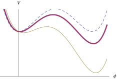
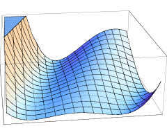
Figure 1: A symmetric potential (dashed line) with a small symmetry breaking term leads to the potential of the purple form. The energy difference between the two minima is $\epsilon$. The lowest line represents the case of a large $\epsilon$. The direction of $\Phi$ field is perpendicular to this diagram.

Figure 2: A panoramic view of the potential in $\phi-\Phi$ plane (Fig.1 is a slice of it). It demonstrates that both the width and the height of the barrier will increase as $\Phi$ augments.

And the approximate expression for B is

$$B=\frac{27\pi^{2}S_{1}^{4}}{2\epsilon^{3}}\simeq\frac{\pi^{2}\mu^{12}}{6\epsilon^{3}\alpha^{4}},$$ (34)

and we draw the diagram of $\Gamma/H^{4}$ as the function of $\Phi$ in Fig.3.

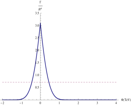
Figure 3: $\Gamma/H^{4}$ as the function of $\Phi$. The dashed line stands for the critical value $\Gamma/H^{4}=9/4\pi$. We take values of $H\simeq TeV$, $m_{\phi}\simeq 2H$ and $\alpha=\lambda=1$. It shows that as $\Phi$ decreases $\Gamma/H^{4}$ remains extremely small and then increases suddenly, which guarantee the universe nucleated and thermalized throughout, and the large void problem will also be settled.

From the diagram, we see that in this special example $\Phi_{ep}\simeq 0.5TeV\simeq\frac{1}{4}m_{\phi}$. And for certain potential with $\Phi_{ep}\simeq\frac{1}{m}\frac{m_{\phi}}{\sqrt{\lambda}}$ we will get $\frac{2}{3}\ln m$ additional e-foldings. If we consider other form of potential, the barrier along $\phi$ direction is the form of trigonometric function, and the height of it is some kind of proportional to the value of $\Phi$ field ($U(\Phi,\phi)=U_{0}(\Phi)\sin\phi$) for example, we could also get the similar results.

Appendix B Time Dependence Of The Expansion Rate

The reason why we take the initial value of $\Phi$ field to be $\Phi_{\textit{initial}}\sim M_{p}$ is not only $M_{p}$ is a natural characteristic value but also the following ones: As the oscillation takes place in the plane of $\phi=0$ with an energy of $\frac{1}{2}m_{\Phi}^{2}\Phi^{2}$, the Friedmann Equation becomes

$$\frac{3}{8\pi}H^{2}M_{p}^{2}=V(0,0)+\frac{1}{2}m_{\Phi}^{2}\Phi^{2}\simeq V(0,0)+\frac{1}{2}H^{2}\Phi^{2},$$ (35)

the approximation is because of $m_{\Phi}\sim H$. According to this equation we provide Tab.1.

$\Phi(M_{p})$	${V(0,0)}/\frac{1}{2}m_{\Phi}^{2}\Phi^{2}$
0.4	1
0.1	25
$10^{-2}$	2500
$10^{-10}$	$2.5\times 10^{19}$

Table 1: The ratio of potential to kinetic energy in the case of different amplitudes of $\Phi$. When $\Phi$=$\alpha M_{p}$, $V(0,0)/\frac{1}{2}m_{\Phi}^{2}\Phi^{2}=\frac{1}{4\alpha^{2}}-1$. The potential energy becomes dominant as the amplitude of $\Phi$ decreases.

The table indicates that as long as $\Phi_{\textit{initial}}\lesssim M_{p}$, the Hubble parameter will basically remain almost constant throughout although the field $\Phi$ changes its amplitude by many $\sim 17$ orders during the inflation.

Anyway, in the event that $\Phi_{\textit{initial}}\gtrsim M_{p}$, with the stage of $\frac{1}{2}m_{\Phi}^{2}\Phi^{2}>V(0,0)$ at the beginning the $\Phi$-oscillation dominates and there would be an interval of matter-dominated expansion until the amplitude of $\Phi$ decreases to $\sqrt{2V(0,0)}/m_{\Phi}$, the energy of $\Phi$ becomes subdominant to $V(0,0)$. In this case, the hubble parameter first decreases approximately $\sim\frac{2}{3t}$, then remains approximately constant.

Bibliography

Bibliography

- [1] A. Linde, “Inflationary Cosmology,” Lect. Notes Phys. 738, 1 (2008) [arXiv:0705.0164 [hep-th]].
- [2] L. McAllister and E. Silverstein, “String Cosmology: A Review,” Gen. Rel. Grav. 40, 565 (2008) [arXiv:0710.2951 [hep-th]].
- [3] B. A. Bassett, S. Tsujikawa and D. Wands, “Inflation dynamics and reheating,” Rev. Mod. Phys. 78, 537 (2006) [arXiv:astro-ph/0507632].
- [4] G. Dvali and S. Kachru, “New old inflation,” arXiv:hep-th/0309095.
- [5] G. Dvali and S. Kachru, “Large scale power and running spectral index in new old inflation,” arXiv:hep-ph/0310244.
- [6] A. D. Linde, “Hybrid inflation,” Phys. Rev. D 49, 748 (1994) [arXiv:astro-ph/9307002].
- [7] G. Dvali, A. Gruzinov and M. Zaldarriaga, “A New Mechanism for Generating Density Perturbations from Inflation,” astro-ph/0303591; G. Dvali, A. Gruzinov and M. Zaldarriaga, “Cosmological Perturbations from Inhomogeneous Reheating, Freeze-Out, and Mass Domination,” astro-ph/0305548; M. Zaldarriaga, “Non-Gaussianities in Models with a Varying Inflaton Decay Rate,” astro-ph/0306006.
- [8] L. Kofman, “Probing String Theory with Modulated Cosmological Fluctuations,” astro-ph/0303614.
- [9] R. Easther, J. Khoury and K. Schalm, “Tuning locked inflation: Supergravity versus phenomenology,” JCAP 0406, 006 (2004) [arXiv:hep-th/0402218].
- [10] E. J. Copeland and A. Rajantie, “The end of locked inflation,” JCAP 0502, 008 (2005) [arXiv:astro-ph/0501668].
- [11] A. H. Guth, “The Inflationary Universe: A Possible Solution To The Horizon And Flatness Problems,” Phys. Rev. D 23, 347 (1981).
- [12] K. Dimopoulos and M. Axenides, “Hybrid inflation without flat directions and without primordial black holes,” JCAP 0506 (2005) 008 [arXiv:hep-ph/0310194].
- [13] S. R. Coleman, “The Fate Of The False Vacuum. 1. Semiclassical Theory,” Phys. Rev. D 15, 2929 (1977) [Erratum-ibid. D 16, 1248 (1977)].
- [14] C. G. . Callan and S. R. Coleman, “The Fate Of The False Vacuum. 2. First Quantum Corrections,” Phys. Rev. D 16, 1762 (1977).
- [15] S. R. Coleman and F. De Luccia, “Gravitational Effects On And Of Vacuum Decay,” Phys. Rev. D 21, 3305 (1980).
- [16] S. Coleman, Phys. Rev. D 15, 2929 (1977); M. B. Voloshin, I. Yu. Kobzarev, and L. B. Okun, Yad. Fiz 20, 1229 (1974) [Sov. J. Nucl. Phys., 20, 644 (1975).
- [17] A. H. Guth and E. J. Weinberg, “Could The Universe Have Recovered From A Slow First Order Phase Transition?,” Nucl. Phys. B 212, 321 (1983).
- [18] M. S. Turner, E. J. Weinberg and L. M. Widrow, “Bubble nucleation in first order inflation and other cosmological phase transitions,” Phys. Rev. D 46, 2384 (1992).
- [19] D. La and P. J. Steinhardt, “Bubble Percolation in Extended Inflationary Models,” Phys. Lett. B 220, 375 (1989).
- [20] D. La, P. J. Steinhardt and E. W. Bertschinger, “Prescription For Successful Extended Inflation,” Phys. Lett. B 231, 231 (1989).
- [21] P. J. Steinhardt and F. S. Accetta, “Hyperextended Inflation,” Phys. Rev. Lett. 64, 2740 (1990).
- [22] C. Brans and R. H. Dicke, “Mach’s principle and a relativistic theory of gravitation,” Phys. Rev. 124, 925 (1961).
- [23] A. D. Linde, “Eternal extended inflation and graceful exit from old inflation without Jordan-Brans-Dicke,” Phys. Lett. B 249, 18 (1990).
- [24] F. C. Adams and K. Freese, “Double field inflation,” Phys. Rev. D 43, 353 (1991).
- [25] E. J. Copeland, A. R. Liddle, D. H. Lyth, E. D. Stewart and D. Wands, “False vacuum inflation with Einstein gravity,” Phys. Rev. D 49 (1994) 6410 [arXiv:astro-ph/9401011].
- [26] M. Axenides and K. Dimopoulos, “Hybrid dark sector: Locked quintessence and dark matter,” JCAP 0407 (2004) 010 [arXiv:hep-ph/0401238].
- [27] R. Allahverdi, A. Jokinen and A. Mazumdar, “Sub-eV Hubble scale inflation within gauge mediated supersymmetry arXiv:hep-ph/0610243.
- [28] R. Allahverdi, K. Enqvist, J. Garcia-Bellido and A. Mazumdar, “Gauge invariant MSSM inflaton,” Phys. Rev. Lett. 97 (2006) 191304 [arXiv:hep-ph/0605035].
- [29] R. Allahverdi, A. Kusenko and A. Mazumdar, “A-term inflation and the smallness of the neutrino masses,” JCAP 0707 (2007) 018 [arXiv:hep-ph/0608138].
- [30] R. Allahverdi, K. Enqvist, J. Garcia-Bellido, A. Jokinen and A. Mazumdar, “MSSM flat direction inflation: slow roll, stability, fine tunning and reheating,” JCAP 0706 (2007) 019 [arXiv:hep-ph/0610134].
- [31] K. Enqvist and A. Mazumdar, “Cosmological consequences of MSSM flat directions,” Phys. Rept. 380 (2003) 99 [arXiv:hep-ph/0209244].
- [32] A. Mazumdar, “MSSM inflaton: SUSY dark matter and LHC,” arXiv:0812.1859 [hep-ph].
- [33] D. H. Lyth, “Can the curvaton paradigm accommodate a low inflation scale,” Phys. Lett. B 579 (2004) 239 [arXiv:hep-th/0308110].
- [34] K. Dimopoulos, D. H. Lyth and Y. Rodriguez, “Low scale inflation and the curvaton mechanism,” JHEP 0502 (2005) 055 [arXiv:hep-ph/0411119].
- [35] Y. Rodriguez, “Low scale inflation and the immediate heavy curvaton decay,” Mod. Phys. Lett. A 20 (2005) 2057 [arXiv:hep-ph/0411120].
- [36] G. Dvali, A. Gruzinov and M. Zaldarriaga, “A new mechanism for generating density perturbations from inflation,” Phys. Rev. D 69 (2004) 023505 [arXiv:astro-ph/0303591].
- [37] L. Kofman, “Probing string theory with modulated cosmological fluctuations,” arXiv:astro-ph/0303614.
- [38] K. Freese and D. Spolyar, “Chain inflation: ’Bubble bubble toil and trouble’,” JCAP 0507, 007 (2005) [arXiv:hep-ph/0412145].
- [39] K. Freese, J. T. Liu and D. Spolyar, “Inflating with the QCD axion,” Phys. Rev. D 72, 123521 (2005) [arXiv:hep-ph/0502177].
- [40] S. Watson, M. J. Perry, G. L. Kane and F. C. Adams, “Inflation without inflaton(s),” JCAP 0711, 017 (2007) [arXiv:hep-th/0610054].
- [41] Q. G. Huang, “Simplified Chain Inflation,” JCAP 0705, 009 (2007) [arXiv:0704.2835 [hep-th]].
- [42] D. Chialva and U. H. Danielsson, “Chain inflation revisited,” JCAP 0810, 012 (2008) [arXiv:0804.2846 [hep-th]].
- [43] A. Ashoorioon, K. Freese and J. T. Liu, “Slow nucleation rates in Chain Inflation with QCD Axions or Monodromy,” arXiv:0810.0228 [hep-ph].
- [44] A. Ashoorioon and K. Freese, “Gravity Waves from Chain Inflation,” arXiv:0811.2401 [hep-th].
- [45] D. Chialva and U. H. Danielsson, “Chain inflation and the imprint of fundamental physics in the CMBR,” arXiv:0809.2707 [hep-th].
- [46] R. Easther, “Folded inflation, primordial tensors, and the running of the scalar arXiv:hep-th/0407042.
- [47] C. P. Burgess, R. Easther, A. Mazumdar, D. F. Mota and T. Multamaki, “Multiple inflation, cosmic string networks and the string landscape,” JHEP 0505, 067 (2005) [arXiv:hep-th/0501125].
- [48] A. Ashoorioon and A. Krause, “Power spectrum and signatures for cascade inflation,” arXiv:hep-th/0607001.
- [49] A. Ashoorioon, A. Krause and K. Turzynski, “Energy Transfer in Multi Field Inflation and Cosmological Perturbations,” JCAP 0902 (2009) 014 [arXiv:0810.4660 [hep-th]].
- [50] A. Mazumdar, S. Panda and A. Perez-Lorenzana, “Assisted inflation via tachyon condensation,” Nucl. Phys. B 614, 101 (2001) [arXiv:hep-ph/0107058].
- [51] Y. S. Piao, R. G. Cai, X. m. Zhang and Y. Z. Zhang, “Assisted tachyonic inflation,” Phys. Rev. D 66, 121301 (2002) [arXiv:hep-ph/0207143].
- [52] M. Majumdar and A. C. Davis, “Inflation from tachyon condensation, large N effects,” Phys. Rev. D 69, 103504 (2004) [arXiv:hep-th/0304226].
- [53] S. Dimopoulos, S. Kachru, J. McGreevy and J. G. Wacker, “N-flation,” JCAP 0808, 003 (2008) [arXiv:hep-th/0507205].
- [54] R. Easther and L. McAllister, “Random matrices and the spectrum of N-flation,” JCAP 0605, 018 (2006) [arXiv:hep-th/0512102].
- [55] J. Ward, “DBI N-flation,” JHEP 0712, 045 (2007) [arXiv:0711.0760 [hep-th]].
- [56] Y. F. Cai and W. Xue, “N-flation from multiple DBI type actions,” arXiv:0809.4134 [hep-th].
- [57] D. Battefeld, T. Battefeld and A. C. Davis, “Staggered Multi-Field Inflation,” JCAP 0810, 032 (2008) [arXiv:0806.1953 [hep-th]].
- [58] D. Battefeld and T. Battefeld, “Multi-Field Inflation on the Landscape,” arXiv:0812.0367 [hep-th].
- [59] T. Damour and V. F. Mukhanov, “Inflation without slow roll,” Phys. Rev. Lett. 80 (1998) 3440 [arXiv:gr-qc/9712061].