Annular shear of cohesionless granular materials:
from inertial to quasistatic regime

Abstract

Using discrete simulations, we investigate the behavior of a model granular material within an annular shear cell. Specifically, two-dimensional assemblies of disks are placed between two circular walls, the inner one rotating with prescribed angular velocity, while the outer one may expand or shrink and maintains a constant radial pressure. Focusing on steady state flows, we delineate in parameter space the range of applicability of the recently introduced constitutive laws for sheared granular materials (based on the inertial number). We discuss the two origins of the stronger strain rates observed near the inner boundary, the vicinity of the wall and the heteregeneous stress field in a Couette cell. Above a certain velocity, an inertial region develops near the inner wall, to which the known constitutive laws apply, with suitable corrections due to wall slip, for small enough stress gradients. Away from the inner wall, slow, apparently unbounded creep takes place in the nominally solid material, although its density and shear to normal stress ratio are on the jammed side of the critical values. In addition to rheological characterizations, our simulations provide microscopic information on the contact network and velocity fluctuations that is potentially useful to assess theoretical approaches.

I Introduction

Significant progress in the modeling of dense granular flow in the inertial regime has been brought about by the recently introduced viscoplastic laws Pouliquen and Chevoir (2002); GDR MIDI (2004); Forterre and Pouliquen (2008), as identified in experiments and discrete numerical simulations in two-dimensional (2D) da Cruz et al. (2005); Lois et al. (2005); Chevoir et al. (2008) and three-dimensional (3D) Jop et al. (2006); Hatano (2007); Peyneau and Roux (2008) situations.

One typically considers homogeneous assemblies of grains of size $d$ and mass density $\rho_{p}$, under shear stress $\sigma$ and average pressure $P$. Denoting the shear rate as $\dot{\gamma}$, constitutive laws are conveniently expressed as relations between dimensionless quantities: effective friction $\mu^{*}$ ($=\sigma/P$), solid fraction $\nu$, and most noticeably inertial number $I=\dot{\gamma}d\sqrt{\rho_{p}/P}$, thus rescaling various experimental data into a consistent picture. As the ratio of the inertial to shear times, the latter parameter quantifies the inertial effects. For a frictional material, a small value of $I$ ($\leq 10^{-2}$) corresponds to the quasistatic critical state regime, while a large value of $I$ ($\geq 10^{-1}$) corresponds to the collisional regime Goldhirsch (2003). As $I$ increases, solid fraction $\nu$ decreases approximately linearly starting from a maximum value $\nu_{max}=\nu_{c}$ (dynamic dilatancy law), while the effective friction coefficient $\mu^{*}$ increases approximately linearly starting from a minimum value $\mu^{*}_{min}=\tan\phi$ (dynamic friction law). This yields a viscoplastic constitutive law, with a Coulomb frictional term and a Bagnold viscous term.

In the quasistatic regime ($I\to 0$) this approach indicates $\mu^{*}\to\mu^{*}_{min}$ constant, independently on the strain, in steady shear flow. Below this minimum stress ratio, quasistatic strains are possible that are described by elastoplastic models. For large enough shear strains Schofield and Wroth (1968); Wood (1990), a solidlike material approaches the so-called critical state, which coincides with the state of steady shear flow in the limit of $I\to 0$.

Once constitutive laws are obtained on dealing with homogeneous systems, they should be locally applicable to all possible flow geometries. Of course, they are quite unlikely to provide a proper description of some strongly heterogeneous situations occurring when strain is localized near boundaries, in thin layers, on a scale of a few grains. Yet, for smoothly varying stress fields, they might prove sucessful, as was shown e.g., with flows down inclined planes. Those were studied in the absence of lateral walls both experimentally and through discrete simulations (see GDR MIDI (2004) for a review). Then the stress distribution becomes heterogeneous but the effective friction remains constant, so that the situation is comparable to homogeneous flows. More remarkably, a three dimensional version of the constitutive law Jop et al. (2006); de Ryck et al. (2008) was found to model similar flows between lateral walls, which induce truly three-dimensional stress distributions and velocity profiles Jop et al. (2005).

Other simple geometries are the vertical chute and the annular shear GDR MIDI (2004). The present paper investigates the material behavior in the annular (Couette) shear geometry, for which the sample is confined between two rough cylinders and sheared by the rotation of the inner one. The annular shear cell is a classical experimental device to measure the rheological properties of complex fluids, and has been used for granular materials, both in two dimensions Miller et al. (1996); Elliott et al. (1998); Veje et al. (1999); Howell et al. (1999a); Hartley and Behringer (2003) and in three dimensions Tardos et al. (1998); Howell et al. (1999b); Mueth et al. (2000); Klausner et al. (2000); Cain (2001); Losert and Kwon (2001); Bocquet et al. (2002); da Cruz et al. (2002); Mueth (2003); Chambon et al. (2003); Tardos et al. (2003); Utter and Behringer (2004); da Cruz (2004); Daniel et al. (2007); Wang et al. (2008). In this geometry, the stress distribution is well known, as will be detailed in the following: the normal stress is approximately constant while the shear stress strongly decreases away from the inner wall. The decrease of $\mu^{*}$ away from the inner wall then explains the localization of the shear. We may even expect a transition between an inertial flow near the inner wall, where $\mu^{*}\geq\mu^{*}_{min}$, and a quasistatic regime further, which analysis would help understanding shear localization near a wall (influence of shear rate and confining pressure on the width and dilation of shear bands), of interest in industrial conducts Nedderman (1992), geotechnical situations Savage (1989) and tectonophysics Chambon et al. (2006).

Following previous discrete simulations Karion and Hunt (1999); Schollmann (1999); Lätzel et al. (2000); Zervos et al. (2000), we investigate the rheology and the microstructure of granular materials in this geometry. We consider two-dimensional, slightly polydisperse assemblies of cohesionless frictional disks. This allows to vary the shear state and provides access to microscopic information at the scale of the grains and of the contact network, hardly measurable experimentally. We prescribe the shear rate and the pressure, allowing global dilation of the shear cell. To save computation time, we implement periodic boundary conditions. All along this paper, we shall compare our results with the homogeneous shear case da Cruz et al. (2005).

Sec. II is devoted to the description of the simulated system, its preparation and the definition of dimensionless control parameters. Sec. III describes the influence of the shear velocity and of the system scale on the shear localization near the inner wall through the radial profiles of various quantities. Sec. IV shows the validity of the previous constitutive law for inertial regime, and analyzes its limit in quasistatic regime. Sec. V then explains how the constitutive law is able to predict various quantities measured in Sec. III.

Preliminary and complementary results are presented in Koval (2008).

II Simulated systems

II.1 Annular shear

The simulated systems are two dimensional (2D) as indicated in Fig. 1. The granular material is a dense assembly of $n$ dissipative disks of average diameter $d$ and average mass $m$. A small polydispersity of $\pm 20\%$ prevents crystallization.

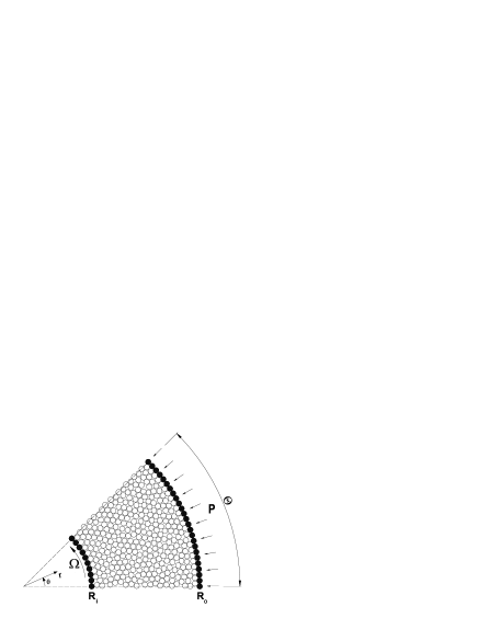
Figure 1: Annular shear geometry (black grains constitute the rough walls).

The granular material is subjected to annular shear between two circular rough walls. The outer wall (radius $R_{o}$) does not rotate, while the inner wall (radius $R_{i}$) moves at the prescribed rotation rate $\Omega$. The wall roughness, which reduces sliding, is made of contiguous glued grains with the same characteristics as the flowing grains (polydispersity and mechanical properties). We call $r$ and $\theta$ the radial and orthoradial directions. $r=R_{i}$ and $r=R_{o}$ respectively correspond to the centers of the grains which compose the inner and outer walls . As the grains of the inner wall form one rigid body, the motion of each of them combines a translation of its center with velocity $\Omega R_{i}\vec{e}_{\theta}$ and a rotation rate $\Omega$.

Since we have not observed any influence of the outer wall on the behavior of the sheared material close to the inner wall for $R_{o}\geq 2R_{i}$, we have set $R_{o}=2R_{i}$, in the results presented in this paper. The geometry is then defined by the sole value of $R_{i}/d$.

An important feature of our discrete simulations is the control of the normal stress exerted by the outer wall on the grains, as done in Zervos et al. (2000). We prescribe $\sigma_{rr}(R_{o})=P$, through the radial motion of the outer wall, given by: $\dot{R}_{o}=(P-\sigma_{rr}(R_{o}))/g_{p}$, where $g_{p}$ is a viscous damping parameter. In steady state, the motion of the outer wall oscillates around a mean value ($\langle\dot{R}_{o}\rangle=0$) corresponding to a prescribed value of the normal stress at this point ($\langle\sigma_{rr}(R_{o})\rangle=P$). Such control of the radial stress is applied in cylinder shear apparatus aimed at studying the behavior of soils near an interface Corfdir et al. (2004). It differs from most experiments and discrete simulations, where the volume is fixed in two dimensions Elliott et al. (1998); Howell et al. (1999a); Karion and Hunt (1999); Lätzel et al. (2000); Lätzel (2003); Utter and Behringer (2004), or dilatancy is possible through the free surface in three dimensions  Tardos et al. (1998); Mueth et al. (2000); Cain (2001); Losert and Kwon (2001); Bocquet et al. (2002); Mueth (2003); Tardos et al. (2003); da Cruz (2004); Daniel et al. (2007); Wang et al. (2008).

We use the standard spring-dashpot contact law described in da Cruz et al. (2005), which introduces the coefficients of restitution $e$ and friction $\mu$, and the elastic stiffness parameters $k_{n}$ and $k_{t}$. Discrete simulations are carried out with standard molecular dynamics method, as in Cundall and Strack (1979); Silbert et al. (2001); Roux and Chevoir (2005); da Cruz et al. (2005); Rognon et al. (2008); Peyneau and Roux (2008). The equations of motion are discretized using Gear’s order three predictor-corrector algorithm Allen and Tildesley (1987).

To decrease the computation time, we have introduced periodic boundary condition along $\theta$, exploiting the angular invariance Cui et al. (2007). This reduces the representation of the annular shear cell to an angular sector $0\leq\theta\leq\Theta$ ($\theta<\pi$) instead of the whole system $0\leq\theta\leq 2\pi$. $\Theta=2\pi/N$, where $N$ is an integer. The description of this method, together with the analysis used to choose the values of $\Theta$ according to the size of the systems, is presented in App. A. The list of simulated geometries is given in Tab. I. We notice that the studied systems are much larger than in previous discrete simulations.

Table 1: List of simulated geometries.

		$n$	$R_{i}/d$	$\Theta/2\pi$
	$R_{25}$	$1500$	$25$	$1/4$
	$R_{50}$	$3100$	$50$	$1/8$
	$R_{100}$	$8000$	$100$	$1/12$
	$R_{200}$	$15700$	$200$	$1/24$

II.2 Dimensional analysis

In our discrete simulations, the system is completely described by a list of independent parameters associated to the grains and to the shear state. As a way to reduce the number of parameters, it is convenient to use dimensional analysis, which guarantees that all the results can be expressed as relations between dimensionless quantities.

The grains are described by their size $d$ and mass $m$, their coefficients of restitution $e$ and friction $\mu$, and their elastic stiffness parameters $k_{n}$ and $k_{t}$. It was shown in previous discrete simulations Silbert et al. (2001); Campbell (2002); da Cruz et al. (2005), that $k_{t}/k_{n}$ and $e$ have nearly no influence on dense granular flows. Consequently, $k_{t}/k_{n}$ was fixed to $0.5$ and $e$ was fixed to $0.1$. The influence of $\mu$, especially near $\mu=0$, has been shown in da Cruz et al. (2005). In this paper, we restrict our analysis to the value $\mu=0.4$, except for the discussion of the constitutive law where the case of frictionless grains ($\mu=0$) will be also analyzed. Results for other values of $\mu$ may be found in Koval (2008).

The shear state is described by the prescribed normal stress on the outer wall $P$, the rotation rate of the inner wall $\Omega$, the radius $R_{i}$ and $R_{o}$ of the two walls, and the viscous damping parameter $g_{p}$. We have not observed any influence of $g_{p}$, once the shear zone is localized near the inner wall and separated by a relatively thick layer of material from the outer wall. The dimensionless number $g_{p}/\sqrt{mk_{n}}$ remains of order $0.1$ in all our simulations, so that the time scale of the fluctuations of $R_{o}$ is imposed by the material rather than the wall, and that the wall sticks to the material. Consequently, the shear state is described by the geometric parameters $R_{i}/d$ ($R_{o}=2R_{i}$), and by the dimensionless tangential velocity of the inner wall (also called shear velocity):

$$V_{\theta}=\frac{\Omega R_{i}}{d}\sqrt{\frac{m}{P}},$$ (1)

which is similar to the notion of inertial number, but at the scale of the whole system. A small value of $V_{\theta}$ corresponds to the quasistatic regime, while a large value corresponds to the collisional regime. Seven values of $V_{\theta}$ have been studied systematically for all systems: $0.0025$, $0.025$, $0.25$, $0.5$, $1.0$, $1.5$ and $2.5$. The value $0.00025$ was also considered in a few cases.

Moreover the stress scales $k_{n}$ and $P$ may be compared through the dimensionless number $\kappa=k_{n}/P$. Let us call $h$ the normal deflection of the contact (or apparent interpenetration of undeformed disks). Being inversely proportional to the relative deflection $h/d$ of the contacts for a confining stress $P$, $\kappa$ is called contact stiffness number da Cruz et al. (2005). A large value corresponds to rigid grains, while a small value corresponds to soft grains. It was shown da Cruz et al. (2005) that it has no influence on the results once it exceeds $10^{4}$, which is the value chosen in all our discrete simulations (rigid grain limit).

In the following (both text and figures), the length, mass, time and stress are made dimensionless by $d$, $m$, $\sqrt{m/P}$ and $P$, respectively.

Table II gives the list of material parameters.

Table 2: List of material parameters.

	polydispersity	$\mu$	$e$	$k_{t}/k_{n}$	$\kappa$
	$\pm 20\%$	$0.4$	$0.1$	$0.5$	$10^{4}$

II.3 Steady shear states

For a given sample, the first step consists in depositing the grains without contact and at rest between the two distant walls. Applying a normal stress at the outer wall, we compress the assembly of grains, considering first that they are frictionless ($\mu=0$), so as to get a very dense initial state. Except near the walls, its solid fraction is close to $0.85$, near the random close packing of slightly polydispersed disks Combe (2002). When the granular material supports completely the applied normal stress, the grains are at rest and the dense system is ready to be sheared. We start to shear the material (now considering that the grains are frictional) imposing the rotation of the inner disk. After a transient, the system reaches a steady state, characterized by constant time-averaged profiles of solid fraction, velocity and stress. In practice, the stabilization of the profiles depends on the considered variable. If we take the inner wall displacement $V_{\theta}\Delta t$ (where $\Delta t$ is the simulation time) as a shear length parameter, the stresses usually present a short transient on a distance around $V_{\theta}\Delta t\leq 5$. However, the stabilization of the solid fraction rather requires $V_{\theta}\Delta t\approx 50$, mostly because of the very dense initial state. Consequently we consider that the condition to reach a steady state is $V_{\theta}\Delta t\geq 100$. This procedure provides an initial state with a shear velocity $V_{\theta}$. As a way to guarantee an initial state consistent for the comparisons between discrete simulations with different $V_{\theta}$, the procedure is first applied with the highest value of $V_{\theta}$, and then $V_{\theta}$ is progressively decreased.

In steady state, we consider that the statistical distribution of the quantities of interest (structure, velocities, forces…) are independent of $t$ and $\theta$, so that we average both in space (along $\theta$) and in time (considering $200$ time steps distributed over the distance $V_{\theta}\Delta t\geq 200$). Then we calculate the profiles of solid fraction, velocity and stress components according to the averaging procedure described in App. B.

Beyond the number of acquisition points, the consistency of the averaged values depends on the shear strain accumulated during the acquisition of data. We concentrate our interest on the region where the system may be considered in a steady state, which occurs at large enough shear strain. Based on the observation of the transients, we consider that this is true when $\dot{\gamma}\Delta t\geq 10$. Because of the strain localization, the region of interest is located near the inner wall and limited to $R_{i}\to R_{i}+R_{steady}$ where the value of $R_{steady}$ is given in Tab. III.

Table 3: Limit of the steady state region. Minimum and maximum values correspond to global quasistatic regime and to $V_{\theta}=2.5$ respectively.

		$R_{steady}$
	$R_{25}$	$7-17$
	$R_{50}$	$9-25$
	$R_{100}$	$13-35$
	$R_{200}$	$18-52$

III Localized shear states

In this section, we show the shear localization near the inner wall through the radial profiles of different quantities. In App. C we focus on internal variables associated to the contact network Radjaï and Roux (2004); Radjaï (2008) (coordination number $Z$ and mobilization of friction $M$) and to the fluctuations of the motion of the grains, translational or rotational. We systematically discuss the influence of $V_{\theta}$.

III.1 Stress field

In steady ($\frac{\partial}{\partial t}=0$) annular shear flows ($\frac{\partial}{\partial\theta}=0$), without radial flow ($v_{r}=0$), continuum mechanics predicts Coleman et al. (1966) a variation of normal stress $\sigma_{rr}$ related to the velocity profile, and a $1/r^{2}$ decrease of the shear stress $\sigma_{r\theta}$ associated to the conservation of the torque:

$$\frac{4\nu}{\pi}\frac{v_{\theta}^{2}}{r} = \frac{\partial\sigma_{rr}}{\partial r}+\frac{\sigma_{rr}-\sigma_{\theta\theta}}{r},$$ (2)

$$\sigma_{r\theta} = S(\frac{R_{i}}{r})^{2},$$ (3)

where $\nu(r)$ and $v_{\theta}(r)$ are the solid fraction and orthoradial velocity profiles, $S$ is the shear stress at the inner wall ($S=\sigma_{r\theta}(R_{i})$) and $\sigma_{ii}$ are positive for compression.

Fig. 2a shows the coarse-grained profiles of the normal stress component $\sigma_{rr}$ in geometry $R_{50}$ for different wall velocities $V_{\theta}$, while Fig. 2b shows the ratio between the orthonormal and the normal stresses $\frac{\sigma_{rr}}{\sigma_{\theta\theta}}$. The normal stress $\sigma_{rr}$ is nearly constant and equal to the confining pressure $P$. The $\partial\sigma_{rr}/\partial r$ term in the momentum equation (2) smoothes the $\sigma_{rr}$ profile, which might explain the absence of fluctuations of $\sigma_{rr}$. A crude estimate of the centrifugal effects may be given, if the last term of equation (2) is neglected, and, anticipating on Sec. III.2 and Sec. III.3, a constant solid fraction $\nu\simeq 0.8$ is assumed and an exponential velocity profile $v_{\theta}(r)=V_{\theta}\exp\left(-(r-R_{i})/\ell\right)$, with $\ell$ between $2$ and $6$:

$$\mid\sigma_{rr}(R_{i})-1\mid\leq\frac{2\pi\nu R_{i}}{\ell}V_{\theta}^{2}.$$ (4)

Consequently, for $R_{i}=50$, $\mid\sigma_{rr}(R_{i})-1\mid\leq 0.05$ for $V_{\theta}=1$ and $\ell=5$. For $V_{\theta}=2.5$, the centrifugal effects might become significant, however it has not been observed.

The radial $\sigma_{rr}$ and orthoradial $\sigma_{\theta\theta}$ stresses are nearly equal for $r-R_{i}\lesssim 10$. This has already been observed in other configurations (plane shear da Cruz et al. (2005); Lois et al. (2005); Peyneau and Roux (2008) within less than $5\%$, inclined plane Silbert et al. (2001); da Cruz (2004); Lois et al. (2005)), and was previously reported in annular shear Lätzel et al. (2000); Lätzel (2003). This very small normal stress difference is not explained yet. The fluctuations of $\sigma_{\theta\theta}$ for $r-R_{i}\gtrsim 15$ probably reflect the frozen disorder beyond the steady zone, where the material is much less deformed than closer to the inner wall, so that the time averaging is unsufficient. Consequently these fluctuations increase as $V_{\theta}$ decreases.

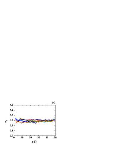
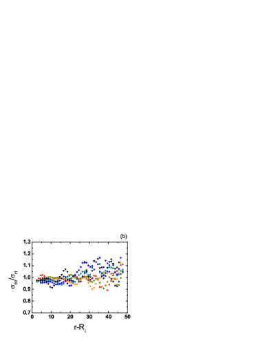
Figure 2: (Color online) (a) Normal stress $\sigma_{rr}(r)$ and (b) ratio between the normal and the orthonormal stresses $\sigma_{\theta\theta}/\sigma_{rr}(r)$ profiles for different shear velocities. ($\blacktriangledown$) $V_{\theta}=0.0025$, (${\color[rgb]{0.00,0.00,1.00}\bullet}$) $V_{\theta}=0.025$, (${\color[rgb]{0.25,0.50,0.50}\blacksquare}$) $V_{\theta}=0.25$, (${\color[rgb]{0.00,0.00,0.50}\blacktriangleright}$) $V_{\theta}=0.5$, (${\color[rgb]{0.50,0.50,0.00}\blacklozenge}$) $V_{\theta}=1.0$, (${\color[rgb]{1.00,0.50,0.00}\blacktriangleleft}$) $V_{\theta}=1.5$, (${\color[rgb]{0.98,0.00,0.00}\blacktriangle}$) $V_{\theta}=2.5$. Geometry $R_{50}$.

The shear stress profiles $\sigma_{r\theta}(r)$ shown in Fig. 3a (for different shear velocity $V_{\theta}$) are consistent with the $1/r^{2}$ decrease of (3). The oscillations about the mean value are due to the material structuration near the inner wall (see Sec. III.3) and to the frozen disorder in the very slowly sheared regions, which is beyond the steady zone.

Fig. 3b shows the dependence of the shear stress at the inner wall $S$ on shear velocity $V_{\theta}$. Below a certain value ($V_{\theta}\lesssim 0.025$), $S$ tends to a finite limit. Consequently, the shear stress profiles $\sigma_{r\theta}(r)$ become independent of $V_{\theta}$. This behavior characterizes the global (that is to say, in the whole system) quasistatic regime, where the stresses (and other state variables) do not depend on the velocity. However, for $V_{\theta}\gtrsim 0.025$, inertial effects become significant and $S$ increases with $V_{\theta}$. Previous works reported a similar dependence of the shear stress on the shear velocity in other configurations (see GDR MIDI (2004) for a review). More specifically, the experimental measurement of the torque as a function of the rotation rate in the annular shear geometry indicates a transition from a rate independent to a rate dependent regime Savage and Sayed (1984); Tardos et al. (1998); Klausner et al. (2000); da Cruz et al. (2002); Daniel et al. (2007). Our results can be approximated by a function like $S=S_{qs}+\alpha V_{\theta}^{\beta}$, where $S_{qs}$ is the global quasistatic limit value, $\alpha$ and $\beta$ are two constants. We notice that $\beta$ is close to $1/2$ rather than $2$ as might be naïvely expected from Bagnold’s rheology. We notice that in the experiment of Tardos et al. (1998), the transition occurs for $V_{\theta}\simeq 0.3$ (after appropriate rescaling), which is not far from what is observed in Fig. 3b. However, we also point out that the $S(V_{\theta})$ curve, here shown for geometry $R_{50}$, in fact depends on the geometry.

Figure 3: (Color online) (a) Shear stress profiles $\sigma_{r\theta}(r)$ (solid lines) and fit according to Eq. (3) (dashed lines) for different wall velocities $V_{\theta}$. (b) Shear stress at the inner wall $S$ as function of $V_{\theta}$ (semi-logarithmic scale). The solid line represents the function: $S=0.26+0.13V_{\theta}^{0.57}$. Geometry $R_{50}$.

III.2 Velocity field

The shear localization near the inner wall is revealed by the strong decrease of velocity profiles $v_{\theta}(r)$ shown on Fig. 4. The decay appears to be nicely approximated by a Gaussian function $v_{\theta}/V_{\theta}=\exp[-a(r-R_{i})-b(r-R_{i})^{2}]$, as shown on Fig. 4. We notice however that there is a sliding velocity for the higher value of $V_{\theta}$ ($2.5$), which is apparent in Fig. 5a. Previous studies in 2D systems Schollmann (1999); Howell et al. (1999b); Lätzel et al. (2000); Losert et al. (2000); Losert and Kwon (2001); Lätzel (2003) found an exponential shape, while a gaussian decay was observed in three dimensional (3D) systems for non spherical or polydispersed grains Mueth et al. (2000). The agreement between the measurement of the velocity profiles in 3D experiment (using 3D MRI velocimetry in the bulk or CIV at the free surface) GDR MIDI (2004) and 2D discrete simulations is satisfactory da Cruz (2004).

The normalization of $v_{\theta}(r)$ by shear velocity $V_{\theta}$ allows to clearly visualize the influence of this latter parameter on the velocity profiles. In the global quasistatic regime ($V_{\theta}\leq 0.025$), there is no influence, while for increasing $V_{\theta}$ above $0.025$, an increase of the localization width is observed, consistently with experimental observations Losert and Kwon (2001).

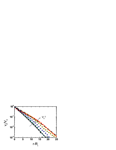
Figure 4: (Color online) Influence of the shear velocity $V_{\theta}$ on the velocity profiles $v_{\theta}(r)$ (semi-logarithmic scale). ($\blacktriangledown$) $V_{\theta}=0.0025$, (${\color[rgb]{0.25,0.50,0.50}\blacksquare}$) $V_{\theta}=0.25$, (${\color[rgb]{0.00,0.00,0.50}\blacktriangleright}$) $V_{\theta}=0.5$, (${\color[rgb]{0.50,0.50,0.00}\blacklozenge}$) $V_{\theta}=1.0$, (${\color[rgb]{1.00,0.50,0.00}\blacktriangleleft}$) $V_{\theta}=1.5$, (${\color[rgb]{0.98,0.00,0.00}\blacktriangle}$) $V_{\theta}=2.5$. The solid line indicates the function $v_{\theta}/V_{\theta}=\exp[-0.34(r-R_{i})-0.0015(r-R_{i})^{2}]$, and the dashed one the function $v_{\theta}/V_{\theta}=\exp[-0.21(r-R_{i})-0.002(r-R_{i})^{2}]$. Geometry $R_{50}$.

The shear rate is equal to $\dot{\gamma}(r)=-r\frac{\partial}{\partial r}(\frac{v_{\theta}(r)}{r})$. We denote $\omega(r)$ the profile of the average angular velocity of the grains. As previously reported in discrete simulations of granular flows da Cruz et al. (2005), the average angular velocity is equal to half the local shear rate (or vorticity) $\omega(r)=-\dot{\gamma}(r)/2$. Oscillations of the average angular velocity are observed in the 3 or 4 first grain layers near the inner wall (Fig. 5), as previously noticed by Lätzel et al. (2000). They may be due to the frustration of the rotation of the flowing grains in contact with the glued grains of the walls (which rotate with angular velocity $\Omega$).

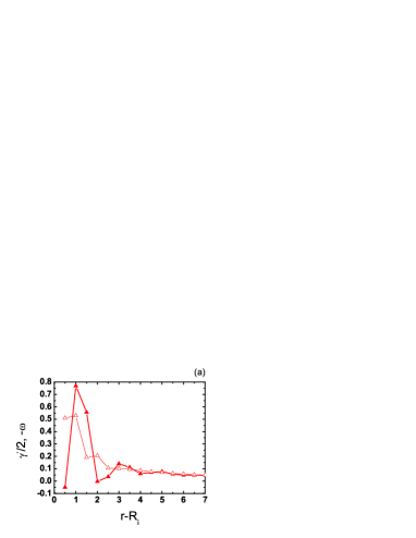
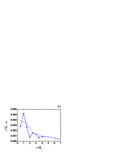
Figure 5: (Color online) Influence of the inner wall on the collapse between the average angular velocity $\omega(r)$ (hollow symbols) and the shear rate $\dot{\gamma}(r)$ (full symbols) (a) $V_{\theta}=2.5$ and (b) $V_{\theta}=0.025$. Geometry $R_{50}$.

III.3 Solid fraction

Fig. 6 shows the solid fraction profiles $\nu(r)$ for $V_{\theta}=0.025$ and $2.5$. In the global quasistatic regime ($V_{\theta}\leq 0.025$), the profile becomes independent of $V_{\theta}$, while a decrease of the solid fraction is observed for increasing $V_{\theta}$. The material is significantly dilated near the inner wall Veje et al. (1999); Schollmann (1999); Lätzel et al. (2000), and is structured in about $5$ layers close to the inner wall, with a higher amplitude for low $V_{\theta}$. This was previously observed in various shear geometries Denniston and Li (1999); Schollmann (1999); Mueth et al. (2000); Ertas et al. (2001); Chevoir et al. (2001). This structuration of the granular material certainly affects the sliding of layers of grains, with significant consequences on the mechanical behavior near the wall. As previously reported Lätzel et al. (2000); Lätzel (2003), independently of the influence of $V_{\theta}$, solid fraction $\nu$ increases toward a value $\nu_{max}$ (close to $0.82$, the solid fraction in the critical state for frictional disks with a similar polydispersity Radjaï and Roux (2004)) away from the inner wall, and remains close to its larger initial value $0.85$ in the region where the material has not been sheared enough.

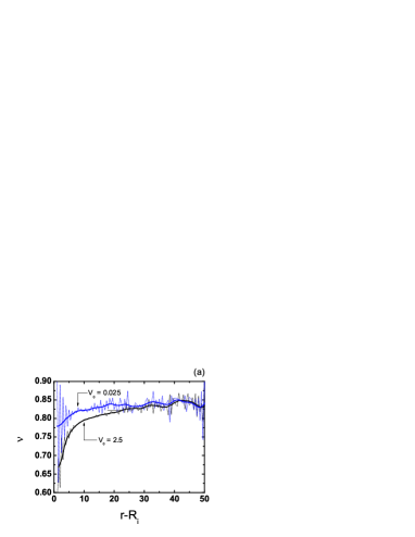
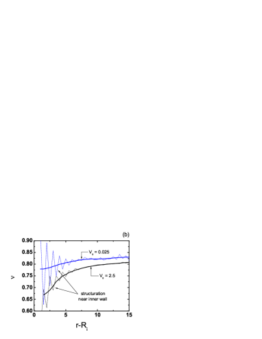
Figure 6: (Color online) Influence of shear velocity $V_{\theta}$ on the structuration near the inner wall. Solid fraction profiles $\nu(r)$ (a) in the whole system and (b) in the region close to the inner wall. The solid line is an average over $3d$, while the dotted line is an average over $0.5d$. Geometry $R_{50}$.

IV Constitutive relations

In Sec. III and App. C, it has been shown that shear velocity $V_{\theta}$, if small enough, no longer influences the radial profiles of various quantities (see Fig. 3, 4, 24 and 25). Then, the whole system is in the quasistatic regime. When $V_{\theta}$ increases, the shear rate $\dot{\gamma}$ increases in the whole sample. Above a certain level of shear rate, inertial effects have significant effect on the material behavior, which characterizes the inertial regime. Considering the shear stress distribution in the annular geometry and the decay of the velocity away from the inner wall, we expect that the inertial zone begins at the inner wall and that its thickness increases when $V_{\theta}$ increases (Fig. 7).

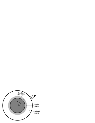
Figure 7: Inertial and quasistatic zones.

In this section, we analyze the relations between different dimensionless quantities in the inertial regime and how they are affected by the transition to the quasistatic regime. We restrict our analysis to large enough shear velocity ($V_{\theta}>0.025$), so that a wide enough inertial zone exists close to the inner wall.

IV.1 Inertial number and mechanical behavior

Discrete simulations of homogeneous plane shear flows  da Cruz et al. (2005) have revealed that the constitutive law of dense granular flows may be described through the dependency of the effective friction $\mu^{*}$ (ratio of shear $\sigma$ to normal $P$ stresses) and of the solid fraction $\nu$ on the inertial number $I=\dot{\gamma}\sqrt{m/P}$ (a 2D equivalent of the definition given in Sec. I), where all the quantities are measured locally. The annular shear flows being heterogeneous, we measure the relations between the local quantities, $\nu(r)$, $\mu^{*}(r)=\sigma_{r\theta}(r)/\sigma_{rr}(r)$ and $I(r)=\dot{\gamma}(r)\sqrt{m/\sigma_{rr}(r)}$ (or $\dot{\gamma}(r)/\sqrt{\sigma_{rr}(r)}$ in dimensionless unit). Each simulation provides dynamic dilatancy and friction laws in a range of inertial number. In the following, we try to analyze the granular material as a continuum, consequently we do not take into account the five first layers where wall structuration effects are significant (see Fig. 5 and Fig. 6).

IV.1.1 Dynamic friction law

In the inertial regime, for $I\gtrsim 0.02$, $\mu^{*}$ increases approximately linearly with $I$ and nearly independently of the geometry (Fig. 8a):

$$\mu^{*}(I)\simeq\mu^{*}_{min}+bI,$$ (5)

with $\mu^{*}_{min}\simeq 0.26$ and $b\simeq 1$. The agreement with the dynamic friction law measured in the homogeneous plane shear geometry is excellent da Cruz et al. (2005); Rognon et al. (2008); Chevoir et al. (2008). In contrast, for lower values of $I$, a deviation from this linear relation is observed, depending on the geometry (Fig. 8b). The effective friction becomes smaller than $\mu^{*}_{min}$, and this deviation increases as $R_{i}$ decreases, that is to say as the stress gradient increases. Reciprocally, as $R_{i}$ increases, that is to say as the stress distribution becomes more homogeneous, the results of the annular geometry tend to the ones of the plane shear geometry. This reveals that the simple relation between effective friction $\mu^{*}$ and inertial number $I$ does not depend on the stress distribution in the inertial regime, and is then quite general (see  da Cruz (2004); Lois et al. (2005) for flows down an inclined plane), while it fails in the quasistatic regime. In plane shear, $\mu^{*}_{min}$ may be considered as the internal friction in the critical state Radjaï and Roux (2004); Peyneau and Roux (2008). This is the maximum value of $\mu^{*}$ supported by the granular material, before it starts to flow quasistatically. With a heterogeneous stress distribution, the granular material is able to flow below this level.

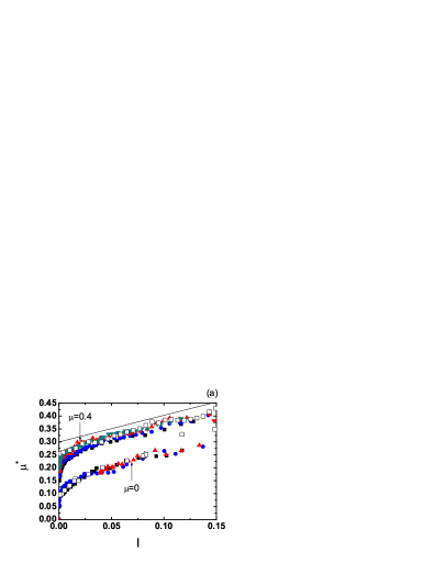
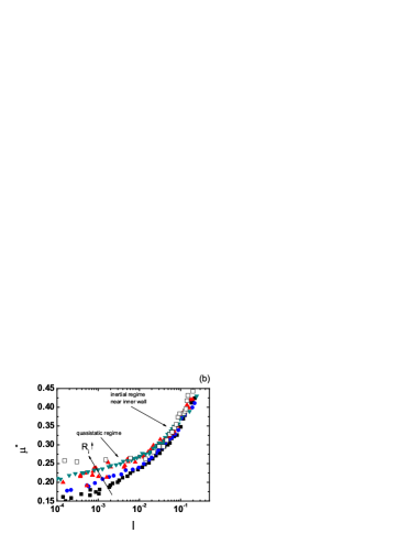
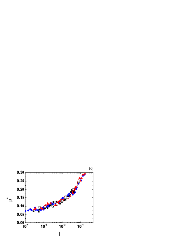
Figure 8: (Color online) Dynamic friction law (a) in linear scale (the solid line indicates a slope $\approx 1$) for particle coefficient of friction $\mu=0$ and $\mu=0.4$. Dynamic friction law in semi-logarithmic scale for (b) $\mu=0.4$ and (c) $\mu=0$. Different geometries: ($\blacksquare$) $R_{25}$, (${\color[rgb]{0.00,0.00,1.00}\bullet}$) $R_{50}$, (${\color[rgb]{0.98,0.00,0.00}\blacktriangle}$) $R_{100}$, (${\color[rgb]{0.25,0.50,0.50}\blacktriangledown}$) $R_{200}$. $V_{\theta}=2.5$. Comparison with plane shear da Cruz et al. (2005) ($\square$).

We call $\lambda_{in}$ the width of the inertial zone. Using Eqn. (3) and (5), we deduce that:

$$\lambda_{in}(V_{\theta},R_{i})=\left(\sqrt{S(V_{\theta},R_{i})/\mu^{*}_{min}}-1\right)R_{i}.$$ (6)

We also conventionally define the width of the shear zone $\lambda_{loc}$ through $v_{\theta}(R_{i}+\lambda_{loc})=V_{\theta}/10$. Fig. 9a and b shows $\lambda_{in}(V_{\theta})$ and $\lambda_{loc}(V_{\theta})$ in geometry $R_{50}$. We notice that $\lambda_{in}$ smoothly increases from zero with $V_{\theta}$, while $\lambda_{loc}$ seems to saturate at a low value for low $V_{\theta}$ (global quasistatic regime) and at a high value for high $V_{\theta}$ (this is related to an apparent velocity discontinuity near the wall, suggesting increasing collisional effects in the first layers), with a sudden increase for $V_{\theta}$ between $0.3$ and $1$. We notice that in the experiment of Losert and Kwon (2001), the shear zone invades the whole gap for high enough $V_{\theta}$.

In a given geometry, for a small enough shear velocity $V_{\theta}$, the inertial zone disappears, and the whole system is in the quasistatic regime. Fig. 10 then shows again that the effective friction $\mu^{*}$ is no more a function of $I$.

Figure 9: (a) Width of the inertial zone $\lambda_{in}$ as a function of $V_{\theta}$, as deduced from Eqn. (6) and Fig. 3a. The solid line represents the function: $\lambda_{in}=50(\sqrt{1+0.5V_{\theta}^{0.57}}-1)$. (b) Width of the localization zone $\lambda_{loc}$ as a function of $V_{\theta}$. Geometry $R_{50}$.

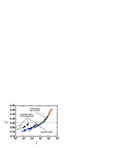
Figure 10: (Color online) Effective friction $\mu^{*}$ as a function of the inertial number $I$ (${\color[rgb]{0.5,0.5,0.5}\bigstar}$) $V_{\theta}=0.00025$, ($\blacktriangledown$) $V_{\theta}=0.0025$, (${\color[rgb]{0.00,0.00,1.00}\bullet}$) $V_{\theta}=0.025$, (${\color[rgb]{0.25,0.50,0.50}\blacksquare}$) $V_{\theta}=0.25$, (${\color[rgb]{0.00,0.00,0.50}\blacktriangleright}$) $V_{\theta}=0.5$, (${\color[rgb]{0.50,0.50,0.00}\blacklozenge}$) $V_{\theta}=1.0$, (${\color[rgb]{1.00,0.50,0.00}\blacktriangleleft}$) $V_{\theta}=1.5$, (${\color[rgb]{0.98,0.00,0.00}\blacktriangle}$) $V_{\theta}=2.5$. The solid line corresponds to $\mu^{*}=0.26$. Geometry $R_{50}$.

IV.1.2 Dynamic dilatancy law

We observe a linear decrease of solid fraction $\nu$ as a function of inertial number $I$, independently of the geometry in the inertial regime (Fig. 11 and 12), and $\nu$ tends to a maximum value $\nu_{max}$, which identifies to the solid fraction in the critical state. We can then write the dynamic dilatancy law:

$$\nu(I)\simeq\nu_{max}-aI,$$ (7)

with $\nu_{max}\simeq 0.82$ and $a\simeq 0.37$. The agreement with the dynamic dilatancy law measured in the homogeneous plane shear geometry is excellent da Cruz et al. (2005); Rognon et al. (2008). However, far from the walls, in the region where the material is less deformed and so remains in its initial dense state, higher values of $\nu$ are observed. Fig. 12 also indicates that the inner wall induces further dilation.

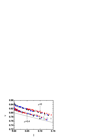
Figure 11: (Color online) Dynamic dilatancy law (the solid line indicate a slope $\approx-0.37$) for different geometries: ($\blacksquare$) $R_{25}$, (${\color[rgb]{0.00,0.00,1.00}\bullet}$) $R_{50}$, (${\color[rgb]{0.98,0.00,0.00}\blacktriangle}$) $R_{100}$, (${\color[rgb]{0.25,0.50,0.50}\blacktriangledown}$) $R_{200}$. Comparison with plane shear da Cruz et al. (2005) ($\square$).

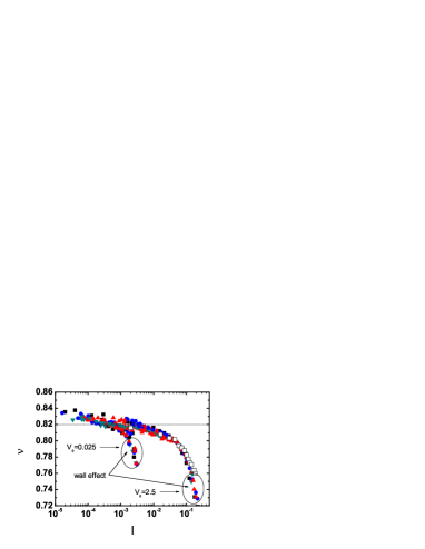
Figure 12: (Color online) Dynamic dilatancy law in semi-logarithmic scale. Different geometries: ($\blacksquare$) $R_{25}$, (${\color[rgb]{0.00,0.00,1.00}\bullet}$) $R_{50}$, (${\color[rgb]{0.98,0.00,0.00}\blacktriangle}$) $R_{100}$, (${\color[rgb]{0.25,0.50,0.50}\blacktriangledown}$) $R_{200}$. Comparison with plane shear da Cruz et al. (2005) ($\square$). The dashed line corresponds to $\nu_{max}=0.82$.

IV.1.3 Frictionless grains

As shown in Fig. 8a and Fig. 11, the microscopic friction coefficient $\mu$ has a significant influence on the constitutive law parameters. Those figures also reveal good agreement with homogeneous shear simulations da Cruz et al. (2005). The solid fraction remains a linearly decreasing function of $I$ (with a fast change in the quasistatic limit). The slope $a$ is not affected, while $\nu_{max}$ increases to $\simeq 0.85$. The dynamic friction law keeps the same tendency but is shifted toward smaller values of friction. The linear approximation with $\mu^{*}_{min}\simeq 0.11$ (Eqn. (5)) fails for $I\leq 0.01$. We notice that the range of validity of the dynamic friction law is much larger than for frictional grains, and that it does not seem to depend on the geometry.

Those differences are likely related to some peculiarities of assemblies of frictionless grains Peyneau and Roux (2008). The quasistatic limit, in such materials, is only approached for much smaller values of $I$ than in the frictional case, and $\mu^{*}_{min}$ is itself considerably lower. As a consequence on may expect a wider inertial zone. Moreover, as the critical solid fraction coincides with the random close packing value Peyneau and Roux (2008), no solid-like region of the system can be prevented from flowing because of its density.

IV.1.4 Comparison with previous studies

The validity of the constitutive law, once suitably generalized to three dimensions, was successfully tested in flows down a heap between lateral walls Jop et al. (2005, 2006). In that case the velocity field, as deduced from numerical computations in which the viscoplastic law was implemented, exhibits a more complex three-dimensional structure. Predicted velocities at the free surface agreed closely with experimental results.

Thus, the applicability of the constitutive law as a relation between local values of non-uniform strain rate and stress fields, which we just established in 2D annular shear flow, was previously checked in the 3D case of a laterally confined gravity-driven flow. The validity of such an approach should be restricted to situations in which the characteristic length for stress or strain rate variations, say $l$, is significantly larger than the grain size. In annular shear, one has $l=R_{i}$, whereas the finite width $w$ of the channel was found in Jop et al. (2005, 2006) to control the gradients, $l=w$. As $R_{i}$, in units of grain diameters, varies between 25 and 200 here, while the interval of $w$ extends between 16.5 and 500 in Jop et al. (2005, 2006), similar levels of heterogeneity are explored.

IV.2 Internal variables

We now discuss how internal variables, which profiles are discussed in App. C, scale with the inertial number $I$, revealing local state laws, consistent with the one measured in homogeneous shear flows.

We observe a relation like $Z=Z_{max}-eI^{f}$ (with $Z_{max}\approx 3$) between coordination number $Z$ and $I$ on Fig. 13, nearly independent of the geometry.

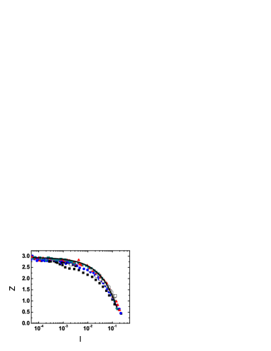
Figure 13: (Color online) Coordination number $Z$ as a function of the inertial number $I$ (the solid line represents the function $Z=2.95-7.65I^{0.65}$) for different geometries. ($\blacksquare$) $R_{25}$, (${\color[rgb]{0.00,0.00,1.00}\bullet}$) $R_{50}$, (${\color[rgb]{0.98,0.00,0.00}\blacktriangle}$) $R_{100}$, (${\color[rgb]{0.25,0.50,0.50}\blacktriangledown}$) $R_{200}$, ($\square$) plane shear da Cruz et al. (2005). $V_{\theta}=2.5$.

We do not observe a general relation between the mobilization of friction $M$ and $I$, but an asymptotic convergence for growing $R_{i}$ toward a relation $M\approx gI^{h}$ (Fig. 14). For this quantity, there is no satisfactory agreement with the homogeneous shear case.

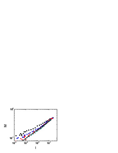
Figure 14: (Color online) Mobilization of friction $M$ as a function of the inertial number $I$ (the solid line represents the function $M=0.73I^{0.29}$ for different geometries: ($\blacksquare$) $R_{25}$, (${\color[rgb]{0.00,0.00,1.00}\bullet}$) $R_{50}$, (${\color[rgb]{0.98,0.00,0.00}\blacktriangle}$) $R_{100}$, (${\color[rgb]{0.25,0.50,0.50}\blacktriangledown}$) $R_{200}$. $V_{\theta}=2.5$.

We analyse the fluctuations of orthoradial velocity $\delta v_{\theta}$ normalized by the natural scale $\dot{\gamma}$ as a function of $I$ (Fig. 15). In the quasistatic regime, the development of collective and intermittent motions (see Mueth (2003); Chambon et al. (2003) in annular shear and  Mills et al. (2008) for a recent review) explain the increase of these relative fluctuations. For higher values of the inertial number $I$, we observe that $\delta v_{\theta}/\dot{\gamma}\rightarrow 1$. On the whole, we propose to describe the dependency by the equation $\delta v_{\theta}/\dot{\gamma}=1+cI^{-d}$ (Fig. 15). Experimental results Mueth et al. (2000); Bocquet et al. (2002) show that $\delta v\varpropto\dot{\gamma}^{0.4}$. Dividing this relation by $\dot{\gamma}$, we get an exponent equal to $-0.6$, close to exponent $d=-0.7$, deduced from the previous fit.

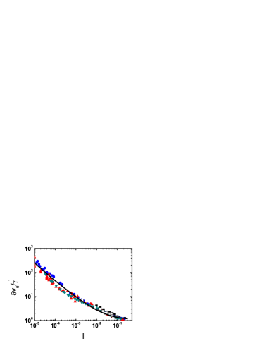
Figure 15: (Color online) Relative fluctuations as a function of the inertial number $I$ (the solid line represents the function $\delta v_{\theta}/(\dot{\gamma}d)=1+0.07I^{-0.7}$). ($\blacksquare$) $R_{25}$, (${\color[rgb]{0.00,0.00,1.00}\bullet}$) $R_{50}$, (${\color[rgb]{0.98,0.00,0.00}\blacktriangle}$) $R_{100}$, (${\color[rgb]{0.25,0.50,0.50}\blacktriangledown}$) $R_{200}$, $\square$ plane shear da Cruz et al. (2005). $V_{\theta}=2.5$.

V Consequences for the shear localization and the macroscopic behavior

Using the constitutive law established in Sec. IV, we now show that it is possible to understand some observations described in Sec. III.

Still using dimensionless units, since the pressure $P$ is constant in the system and the shear stress is given by Eqn. (3), the dynamic friction law Eqn. (5) provides the following equation for the velocity profile $v_{\theta}(r)$:

$$\frac{\partial}{\partial r}(\frac{v_{\theta}(r)}{r})=\frac{\mu^{*}_{min}}{br}-\frac{SR_{i}^{2}}{br^{3}},$$ (8)

where the shear stress at the inner wall $S$ depends both on $V_{\theta}$ and on $R_{i}$ (see Sec. III.1). As shown from the measurements drawn in Fig. 16b, for a large value of $V_{\theta}$, $S$ is high in small geometries and strongly decreases as $R_{i}$ increases. We now integrate this relation over the range of validity of the dynamic friction law, this is to say in the inertial zone $R_{i}\to R_{in}=R_{i}+\lambda_{in}$, from which we get:

$$v_{\theta}(r)=\frac{SR_{i}^{2}}{2br}+\frac{\mu^{*}_{min}}{b}r\ln(r)+cr.$$ (9)

The constant $c$ is determined by the value of the velocity at the inner wall, called $V^{+}_{\theta}$, which is smaller than $V_{\theta}$, revealing some sliding at the wall as previously noticed (see Sec. III.2).

$$V^{+}_{\theta}=\frac{SR_{i}}{2b}+\frac{\mu^{*}_{min}}{b}R_{i}\ln(R_{i})+cR_{i}.$$ (10)

On the whole, the velocity profile is equal to:

$$v_{\theta}(r)=V^{+}_{\theta}\frac{r}{R_{i}}+r\left[\frac{S}{2b}\left(\left(\frac{R_{i}}{r}\right)^{2}-1\right)+\frac{\mu^{*}_{min}}{b}\ln\left(\frac{r}{R_{i}}\right)\right].$$ (11)

An absolute measurement of $V^{+}_{\theta}$ happens to be difficult, considering the wall effect that disturbs the material behavior in a layer of a few grains near the inner wall (like in Fig. 5 for the shear rate $\dot{\gamma}$). Consequently, we obtain this quantity from a fit, and a comparison with the measured velocity profiles is shown on Fig. 16b. The agreement is excellent, suggesting once more the validity of the dynamic friction law. The sliding increases when $V_{\theta}$ increases and, as shown in Fig. 16b, increases when $R_{i}$ decreases.

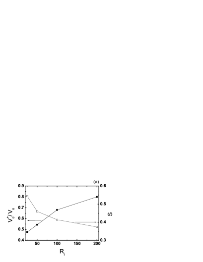
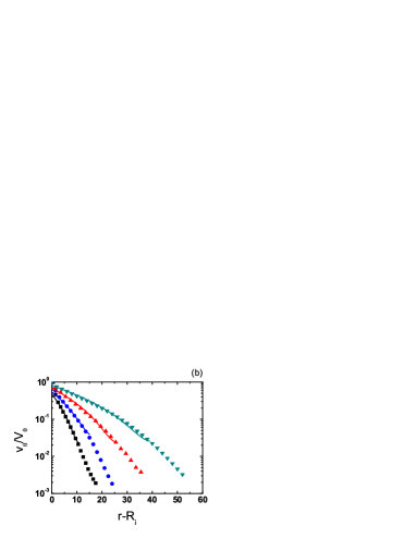
Figure 16: (Color online) (a) Influence of the geometry on ($\blacksquare$) $V^{+}_{\theta}/V_{\theta}$ (fit) and ($\square$) $S$ (measurement) ($V_{\theta}=2.5$). (b) Velocity profiles: comparison between the measurements ($\blacksquare$) $R_{25}$, (${\color[rgb]{0.00,0.00,1.00}\bullet}$) $R_{50}$, (${\color[rgb]{0.98,0.00,0.00}\blacktriangle}$) $R_{100}$, (${\color[rgb]{0.25,0.50,0.50}\blacktriangledown}$) $R_{200}$ and the prediction of Eqn. (11) (solid lines). The velocity profiles are limited to the steady zone $R_{i}\to R_{i}+R_{steady}$ ($V_{\theta}=2.5$).

We now try to predict the $S(V_{\theta})$ relation, which was measured and fitted in Fig. 3b. It is clear that in the global quasistatic limit, as $V_{\theta}\to 0$, $S\to\mu^{*}_{min}$. We now write a boundary condition at the limit of the inertial zone $R_{in}$. Having used the dynamic friction law Eqn. (5), we necessarily have $\dot{\gamma}(R_{in})=0$, as appears in the fitted curve in Fig 16b. Then, beyond $R_{in}$, if this dynamic friction law was still valid , $\dot{\gamma}(r)$ would be strictly equal to zero, so that $v_{\theta}(r)$ would be equal to $Cr$, with a constant $C$. The sole possibility is $C=0$ since the velocity must be equal to zero at the outer wall. We conclude that $v_{in}=v_{\theta}(R_{in})=0$. This conclusion is wrong, as it is clear in Fig 16b, and has already been discussed: the dynamic friction law fails in the quasistatic regime, and we shall come back to this point just after the discussion of the $S(V_{\theta})$ relation. The previous assumption writes:

$$0=V^{+}_{\theta}\frac{R_{in}}{R_{i}}+R_{in}\left[\frac{S}{2b}\left(\left(\frac{R_{i}}{R_{in}}\right)^{2}-1\right)+\frac{\mu^{*}_{min}}{b}\ln\left(\frac{R_{in}}{R_{i}}\right)\right].$$ (12)

Since Eqn. (6) is equivalent to $R_{in}/R_{i}=\sqrt{S/\mu^{*}_{min}}$, we get the following implicit $S(V^{+}_{\theta})$ relation:

$$\frac{S}{\mu^{*}_{min}}-1-\ln\left(\frac{S}{\mu^{*}_{min}}\right)=\frac{2bV^{+}_{\theta}}{\mu^{*}_{min}R_{i}}.$$ (13)

For simplicity, we take $V^{+}_{\theta}=V_{\theta}$ in the comparison with the measurements, drawn in Fig 17 for two geometries. The agreement is very satisfactory considering the previous simplifying assumptions. With the increase of $R_{i}$, the difference between $V^{+}_{\theta}$ and $V_{\theta}$ decreases, explaining the better results for $R_{200}$. For small $V_{\theta}$, we write $S(V_{\theta})=\mu^{*}_{min}(1+f(V_{\theta}))$. A simple development gives $f\simeq\sqrt{\frac{2b}{\mu^{*}_{min}R_{i}}}\sqrt{V_{\theta}}$. For $R_{i}=50$, $f\simeq 0.55\sqrt{V_{\theta}}$, which is close to the fit $f\simeq 0.5V_{\theta}^{0.57}$ used in Fig. 3b. According to this analysis, $S$ becomes proportional to $V_{\theta}$ for much larger values, not usually accessible.

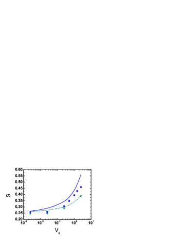
Figure 17: (Color online) Shear stress at the wall $S$ as a function of the wall velocity $V_{\theta}$. Comparison between the measurements: (${\color[rgb]{0.00,0.00,1.00}\bullet}$) $R_{50}$ and (${\color[rgb]{0.25,0.50,0.50}\blacktriangledown}$) $R_{200}$ and the predictions of Eqn. (13). The solid and dashed line respectively indicate the results for $R_{50}$ and $R_{200}.$

We now come back to the limit of the dynamic friction law, Eqn. (5), in the quasistatic limit, as shown in Fig. 8b. A large portion of the velocity profile in the steady quasistatic regime is shown in Fig. 16b. As a first approximation, the velocity can be considered exponential in this region, so that we write:

$$v_{\theta}(r)=v_{in}\exp-\left(\frac{r-R_{in}}{\lambda_{qs}}\right),$$ (14)

with $\lambda_{qs}$ the characteristic length in the quasistatic region, measured in Fig. 18 (which are slightly larger than the one estimated for very small $V_{\theta}$, that is to say when the quasistatic zone invades the system), and $v_{in}$ is not equal to zero contrarily to the previous simple approximation but, using Eqn. (11) to:

$$v_{in}=\sqrt{\frac{S}{\mu^{*}_{min}}}\left(V^{+}_{\theta}+\frac{\mu^{*}_{min}R_{i}}{2b}\left(\ln\left(\frac{S}{\mu^{*}_{min}}\right)-\frac{S}{\mu^{*}_{min}}+1\right)\right).$$ (15)

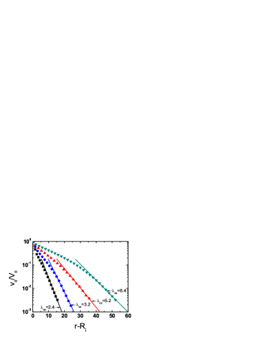
Figure 18: (Color online) Characteristic length $\lambda_{qs}$ obtained from the velocity profiles in the quasistatic zone. Different geometries: ($\blacksquare$) $R_{25}$, (${\color[rgb]{0.00,0.00,1.00}\bullet}$) $R_{50}$, (${\color[rgb]{0.98,0.00,0.00}\blacktriangle}$) $R_{100}$, (${\color[rgb]{0.25,0.50,0.50}\blacktriangledown}$) $R_{200}$. $V_{\theta}=2.5$.

Still using dimensionless units, since the pressure $P$ is constant in the system, we deduce that, for $r\geq R_{in}$, the inertial number is equal to:

$$I(r)=\left(\frac{1}{\lambda_{qs}}+\frac{1}{r}\right)v_{in}\exp-\left(\frac{r-R_{in}}{\lambda_{qs}}\right).$$ (16)

Since $R_{in}\gg\lambda_{qs}$, we may write:

$$I(\mu^{*})\simeq\frac{v_{in}}{\lambda_{qs}}\exp-\frac{R_{i}\sqrt{S/\mu^{*}_{min}}}{\lambda_{qs}}\left(\sqrt{\mu^{*}_{min}/\mu^{*}}-1\right).$$ (17)

from which we obtain:

$$\mu^{*}(I)\simeq\mu^{*}_{min}\left(1-\frac{\lambda_{qs}}{R_{i}\sqrt{S/\mu^{*}_{min}}}\ln\left(\frac{\lambda_{qs}}{v_{in}}I\right)\right)^{-2}.$$ (18)

This prediction is in close agreement with the measurements, as shown in Fig. 19.

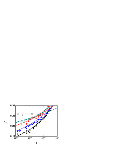
Figure 19: Effective friction $\mu^{*}$ as function of the inertial number $I$, in the quasistatic zone. Comparison between the measurements: ($\blacksquare$) $R_{25}$, (${\color[rgb]{0.00,0.00,1.00}\bullet}$) $R_{50}$, (${\color[rgb]{0.98,0.00,0.00}\blacktriangle}$) $R_{100}$, (${\color[rgb]{0.25,0.50,0.50}\blacktriangledown}$) $R_{200}$, ($\square$) plane shear da Cruz et al. (2005) and the prediction of Eqn. (18) (solid lines). The dashed line indicates $\mu^{*}_{min}=0.26$. $V_{\theta}=2.5$.

VI Conclusion

We first summarize the results presented in this paper, before discussing the questions raised by those conclusions.

As described in Sec. II, we have studied through discrete simulations steady annular shear flows of a model granular material, made of a slightly polydisperse assembly of frictional dissipative disks, prescribing the rotation rate of the inner wall and the pressure exerted by the outer wall, and varying dimensionless shear velocity $V_{\theta}$ and size $R_{i}$ of the system.

The first step (Sec. III) has consisted in measuring various quantities, either global as the dimensionless shear stress at the inner wall $S$ as a function of $V_{\theta}$, or local as the profiles of stress components, velocity, solid fraction and some internal variables (coordination number, mobilization of friction, velocity fluctuations, shown in App. C). This has allowed to distinguish, at the global scale, that is to say as a function of $V_{\theta}$, between rate dependent and rate independent behaviors.

Inspired by our previous rheophysical analysis of homogenous shear flows of disks da Cruz et al. (2005), the second step (Sec. IV) has explored the validity of constitutive law for inertial regime if applied locally in such an heterogeneously sheared material. We have shown that the dynamic friction and dilatancy laws observed in homogeneous shear flows are exactly recovered, when using the local state parameter $I$ called inertial number. Scaling laws for internal variables as function of $I$ have also been observed. This analysis has clearly distinguished an inertial zone close to the inner wall where the constitutive law is relevant and a quasistatic zone away from it, where it fails.

The last step (Sec. V) has explained how it is possible to predict some observations presented in the first step, when using the inertial constitutive law identified in the second step. We have focused on two basic quantities, which are most often discussed in the studies of annular shear flows of granular materials, the macroscopic $S(V_{\theta})$ relation and the microscopic velocity profiles. The satisfactory agreement between the prediction and the measurements should not be surprising, considering the second step. However this analysis has precisely pointed out two important issues, related to boundary conditions in such a heterogeneously sheared system, one at the shearing wall, and the other at the transition between inertial and quasistatic zone.

Close to the inner wall, as previously shown in different configurations, various quantities (solid fraction, ratio of normal stresses, rotation velocity…) present singular behaviors. The translation velocity reveals significant sliding for sufficiently high $V_{\theta}$, even with the large roughness used in this study. We have shown that the value $V_{\theta}^{+}$ of this sliding velocity is an important ingredient for a good prediction. This means that a detailed understanding of the rheophysics of the granular materials in the very first layers near a rough wall is of great relevance. Apart from the characteristics of the granular material itself, the relative influences of $V_{\theta}$, $R_{i}$ and the wall roughness must be taken into account. Comparisons between physical experiments and discrete simulations are described in Koval (2008). Considering the frustration of the particle rotation imposed by the wall, Cosserat models might be adapted to describe this interface zone Tejchman and Wu (1993), as done by Lätzel et al. (2000); Mohan et al. (2002) for annular shear. Another discussion of the boundary condition at the wall is proposed in Artoni et al. (2008).

The transition between inertial and quasistatic zones is a second puzzling issue. Considering the constitutive law identified in homogeneous shear flows, the granular material should reach the so-called critical state in the quasistatic limit (when $I\to 0$), in which it flows rate independently with an effective friction $\tan\phi$ and a solid fraction $\nu_{c}$. Beyond this limit (for $S/P<\tan\phi$ and/or $\nu>\nu_{c}$), the granular material, being in a solid-like state, should not be able to flow. However (apparently unbounded) creep flows are observed in this nominally solid regime. This creeping behavior is well known in free surface flows, where an exponential velocity profile has been clearly evidenced with a characteristic length of the order of one grain diameter Rajchenbach (2000); Khakhar et al. (2001); Komatsu et al. (2001); Crassous et al. (2008). In the annular shear geometry, a similar behavior is observed but the characteristic length increases as $R_{i}$ increases, that is to say as the stress gradient decreases, or as the stress field becomes more homogeneous.

For a sufficiently small $V_{\theta}$, there is no more inertial zone, so that both boundary conditions occur at the same place, the inner wall. Considering the typical values of the parameters in the systems which have been studied experimentally or through discrete simulations, we notice that this corresponds to the usual case. The understanding of such a situation merges the two previous problems: the behavior of a granular material close to an interface and in the quasistatic regime, together with the heterogeneity of the stress field.

The already noticed observation of collective and intermittent motions in this quasistatic regime has driven the development of several rheological models (see Debrégeas and Josserand (2000); Bocquet et al. (2002); Tardos et al. (2003); Lagree and Lhuillier (2006) and Mills et al. (2008) for a recent review): diffusion equation for the fluctuations, transmission of forces at the scale of correlated clusters, two-phase fluid model with order parameter, activation of rearrangements through the fluctuations of velocity or forces, occurring either at the boundary of the inertial zone, or at the inner wall in the global quasistatic limit.

Our understanding is far from complete and requires further studies, merging physical experiments, discrete simulations and theoretical developments. For instance, we have not measured the fabric in the quasistatic zone, although its importance has been clearly evidenced in homogeneous shear Radjaï and Roux (2004); Radjaï (2008). We have not discussed the evolution of the internal variables in the transient regime (evolution from initial to steady state), or in a shear reversal regime Losert and Kwon (2001); Utter and Behringer (2004), as should be qualitatively possible using simplified microscopic description Falk et al. (2008). We have restricted our attention to velocity controlled shear flows, so that it was not possible to study the flow threshold. A specific study of the jamming mechanisms should be performed by controlling the shear stress da Cruz et al. (2002). We have not discussed the influence of the roughness on the interface behavior, for which we refer to Koval (2008). We may also wonder to what extent the conclusions drawn for granular materials differ for other complex fluids made of interacting elements (dense suspensions, foam, emulsions…) Debrégeas et al. (2001); Huang et al. (2005).

Appendix A : Periodic boundary condition

Each grain the center of which is in $(r,\theta)$ with $0\leq\theta\leq\Theta$ is associated to a collection of copies with centers in $r,\theta+k\Theta$ where $k$ is an integer. The corresponding velocities, accelerations and forces are related by rotations of angles $k\Theta$.

Every time a grain moves out of the simulation cell, one of its copies moves in by the opposite boundary, similarly to the usual case of periodic boundary conditions by translation. However the velocities, accelerations and forces are affected by a rotation of $\pm\Theta$.

The situation of the contact of two grains $i$ and $j$ where $\theta_{i}$ is close to $\Theta$ and $\theta_{j}$ is close to zero is described in Fig. 20. More precisely, $i$ is in contact with the copy $j^{\prime}$ of $j$, obtained by rotation of an angle $\Theta$, while $j$ is in contact with $i^{\prime}$ obtained by rotation of $i$ of an angle $-\Theta$. To evaluate the forces acting over grain $i$ we have to use the normal and tangential unit vectors $\vec{n}_{ij^{\prime}}$ (pointing from $i$ to $j^{\prime}$) and $\vec{t}_{ij^{\prime}}$ (such that $({\vec{n}}_{ij^{\prime}},{\vec{t}}_{ij^{\prime}})$ is positively oriented), respectively, and the motion of the grain $j^{\prime}$, while for $j$ we have to use corresponding $\vec{n}_{ji^{\prime}}$ and $\vec{t}_{ji^{\prime}}$ and the motion of $i^{\prime}$. Vector $\vec{n}_{ij^{\prime}}$ is not, as usually, equal to $-\vec{n}_{ji^{\prime}}$, but to its image obtained by rotation of an angle $-\Theta$.

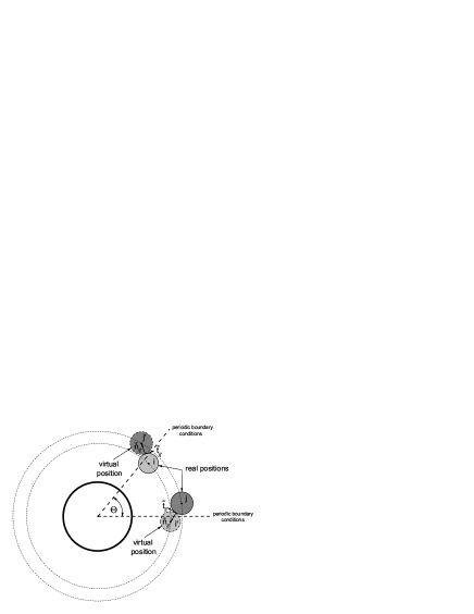
Figure 20: Periodic boundary conditions.

We have measured the influence of the periodic boundary condition comparing the radial profiles of various quantities as a function of $\Theta$ ($\pi/16$, $\pi/8$, $\pi/4$, $\pi/2$, $\pi$ and the whole ring $2\pi$) for the geometry $R_{i}=25$ and $R_{o}=50$. As an example, we show on Fig. 21 the profiles of the orthoradial velocity. As expected, the results are all the more consistent as the value of $\Theta$ increases. In this case, $\Theta=\pi/2$ already gives a very good result.

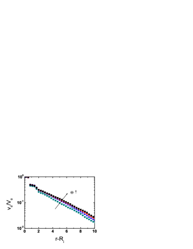
Figure 21: (Color online) Velocity profiles $v_{\theta}(r)/V_{\theta}$ for different values of $\Theta$ (rad). (${\color[rgb]{0.25,0.50,0.50}\bullet}$) $\Theta=\pi/16$, (${\color[rgb]{0.00,0.00,1.00}\blacktriangle}$) $\Theta=\pi/8$, (${\color[rgb]{0.98,0.00,0.00}\blacktriangledown}$) $\Theta=\pi/2$, ($\blacksquare$) $\Theta=2\pi$. $R_{i}=25$, $R_{o}=50$, $V_{\theta}=2.5$.

We quantify the deviations of the velocity profiles $v_{\theta}(r)$ by means of an indicator of relative error. The velocity tends to zero as the distance from the inner wall. To avoid inconsistencies due to values close to zero in the frame of the usual definition of relative error, and to give more weight to the values close to the inner wall, we propose to calculate the relative error over variable $F_{\Theta}(r)=V_{\theta}-v_{\theta}(r,\Theta)$ :

$$\ \varepsilon(\Theta)=\frac{1}{R_{o}-R_{i}}\int^{R_{o}}_{R_{i}}|{\frac{F_{\Theta}(r)-F_{2\Theta}(r)}{F_{2\Theta}(r)}}|dr.$$ (19)

$\varepsilon(\Theta)$ is simply the sum over the whole geometry of the relative error of the variable $F$ for a certain value of $\Theta$ compared to the result for a system twice as large ($2\Theta$).

On Fig. 22a, we observe a clear decrease of the error indicator $\varepsilon(\Theta)$ as we increase the value of $\Theta$ for the smallest geometry ($R_{i}=25$ and $R_{o}=50$). The same analysis for a larger geometry ($R_{i}=100$ and $R_{o}=200$) shows better results for smaller values of $\Theta$. This shows that the influence of $\Theta$ on the results depends on the size of the system. We try to relate both parameters in Fig. 22b, where we plot $\varepsilon(\Theta)$ as a function of the angular sector length at the inner wall ($\Theta R_{i}$). We observe that a good accuracy of the results can be achieved with a length $\Theta R_{i}\geq 40$ for geometries with $R_{i}\geq 25$. Based on this consideration, we have chosen the values of $\Theta$ for each of our geometries (Tab. I).

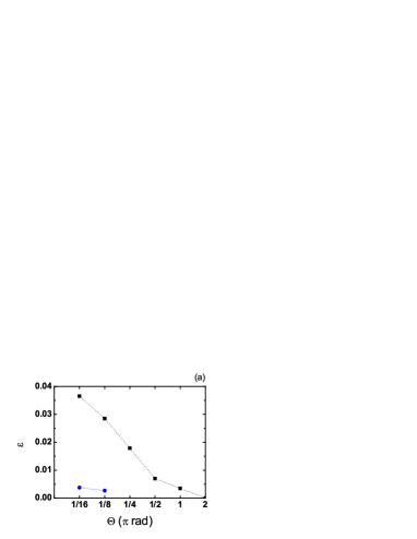
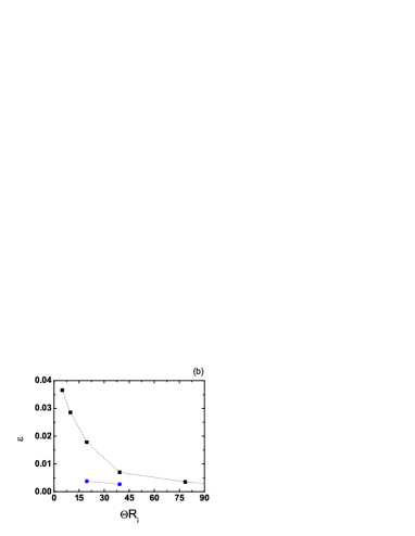
Figure 22: (Color online) Relative error $\varepsilon$ on the orthoradial velocity $v_{\theta}$ ($V_{\theta}=$ 2.5), (a) as function of $\Theta$, (b) as function of the inner wall length $\Theta R_{i}$. ($\blacksquare$) $R_{i}=25$ and $R_{o}=50$, (${\color[rgb]{0.00,0.00,1.00}\bullet}$) $R_{i}=100$ and $R_{o}=200$.

Appendix B : Averaging method

Considering the revolution symmetry of our system, the radial profiles of different quantities (orthoradial velocity $v_{\theta}(r)$, coordination number $Z(r)$, etc.) are obtained by an averaging procedure over coordinate $\theta$ along the coordinate $r$ (Fig. 23). To each of the $n$ grains $i$ are associated different scalar quantities $G^{i}$. We define a weight function $\psi_{i}(r)$ as the intercept angle defined on Fig. 23 ($\cos(\psi_{i}(r)/2)=(r^{2}+r_{i}^{2}-d_{i}^{2}/4)/(2rr_{i})$ for a disk of diameter $d_{i}$). Some variables, like solid fraction $\nu$, are averaged over the whole space, while others, like the coordination number $Z$, have no sense outside the grain space. This leads to the two following definitions of the average :

$$<G>(r)=\frac{1}{\Theta}\sum_{i=1}^{n}G^{i}\psi_{i}(r),$$ (20)

and :

$$<G>^{\prime}(r)=\frac{\sum_{i=1}^{n}G^{i}\psi_{i}(r)}{\sum_{i=1}^{n}\psi_{i}(r)}.$$ (21)

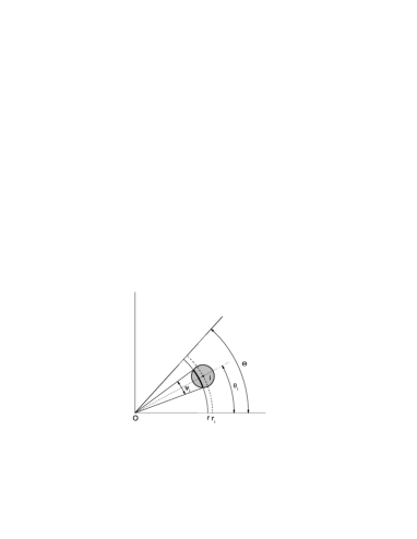
Figure 23: Various quantities associated to a grain $i$.

Applying this principle, we determine the solid fraction profile $\nu(r)$ as follows

$$<\nu>(r)=\frac{1}{\Theta}\sum_{i=1}^{n}\psi_{i}(r),$$ (22)

where the value of $\nu_{i}$ is naturally equal to $1$. This means that $<G>$ and $<G>^{\prime}$ are simply related by the solid fraction: $<G>=<\nu><G>^{\prime}$.

We take into account the variation of vectorial and tensorial quantities inside the grains, when written in the polar basis $\vec{e}_{r}(\phi)=\left(\begin{array}[]{c}\cos\phi\\ \sin\phi\\ \end{array}\right)$ and $\vec{e}_{\theta}=\left(\begin{array}[]{c}-\sin\phi\\ \cos\phi\\ \end{array}\right)$. Hence, the radial profiles of the velocity components are :

$$v_{\alpha}(r)=\frac{1}{\sum_{i=1}^{n}\psi_{i}(r)}\sum_{i=1}^{n}\int^{\theta_{i}+\frac{\psi_{i}}{2}}_{\theta_{i}-\frac{\psi_{i}}{2}}\vec{v}^{i}\cdot\vec{e}_{\alpha}(\phi)d\phi.$$ (23)

The stress tensor of each grain is defined according to Moreau (1997) (with $A^{i}=\pi d_{i}^{2}/4$ the grain area) :

$$\underline{\underline{\sigma}}^{i}=\frac{1}{A^{i}}\left(\sum_{j\neq i}{\vec{F}}_{ij}\otimes{\vec{r}}_{ij}+m_{i}\delta\vec{v}_{i}\otimes\delta\vec{v}_{i}\right).$$ (24)

The first term is associated to the contact forces, and the second one to the velocity fluctuations. The radial profiles of the components of the stress tensor are :

$$\sigma_{\alpha\beta}(r)=\frac{1}{\Theta}\sum_{i=1}^{n}\int^{\theta_{i}+\frac{\psi_{i}}{2}}_{\theta_{i}-\frac{\psi_{i}}{2}}\vec{e}_{\alpha}(\phi)\cdot\underline{\underline{\sigma}}^{i}\cdot\vec{e}_{\beta}(\phi)d\phi.$$ (25)

Since we try to analyze the granular material as a continuum (except for the very first layers near the wall), we consider the coarse-grained variations of the quantities by smoothing the profiles through central moving averages of $3d$ length (if not otherwise indicated). The remaining fluctuations would disappear with an increase of the simulation time $\Delta t$ over which the data are averaged.

Appendix C : Internal variables

Coordination number $Z$ is the average number of contacts per grain. In the inertial regime, the general tendency is a decrease of $Z$ as the shear rate $\dot{\gamma}$ increases (that is to say for increasing $V_{\theta}$ in Fig. 24). For smaller values of $\dot{\gamma}$ (corresponding to smaller values of $V_{\theta}$ or to a larger distance from the inner wall) the coordination number $Z$ approaches a limiting value, slightly above 3. Such a limit is in rough agreement with other numerical observations of the critical state of frictional disks. Ref. Radjaï and Roux (2004) thus reports $Z\simeq 3.6$. The somewhat lower values observed in our case are likely due to the larger strain rates, and to the remaining influence, on the quasistatic region of limited width, of the more agitated inner zone.

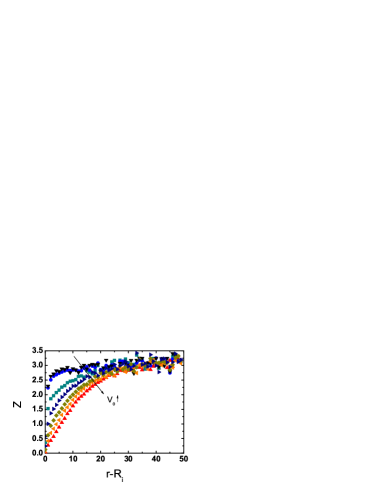
Figure 24: (Color online) Influence of shear velocity $V_{\theta}$ on the coordination number profiles $Z(r)$. ($\blacktriangledown$) $V_{\theta}=0.0025$, (${\color[rgb]{0.00,0.00,1.00}\bullet}$) $V_{\theta}=0.025$, (${\color[rgb]{0.25,0.50,0.50}\blacksquare}$) $V_{\theta}=0.25$, (${\color[rgb]{0.00,0.00,0.50}\blacktriangleright}$) $V_{\theta}=0.5$, (${\color[rgb]{0.50,0.50,0.00}\blacklozenge}$) $V_{\theta}=1.0$, (${\color[rgb]{1.00,0.50,0.00}\blacktriangleleft}$) $V_{\theta}=1.5$, (${\color[rgb]{0.98,0.00,0.00}\blacktriangle}$) $V_{\theta}=2.5$. Geometry $R_{50}$.

We define the mobilization of friction as ratio $M=Z_{s}/Z$, where $Z_{s}$ is the average number of sliding contacts per grain Staron et al. (2002); da Cruz et al. (2005). Fig. 25 shows that $M$ increases as the shear rate increases, whether through an increase of $V_{\theta}$ or a decrease of the distance from the inner wall. We notice that the stabilization of the $M(r)$ profile occurs for $V_{\theta}\leq 0.0025$, a value much smaller than the one required for the stabilization of the other studied quantities ($V_{\theta}\leq 0.025$).

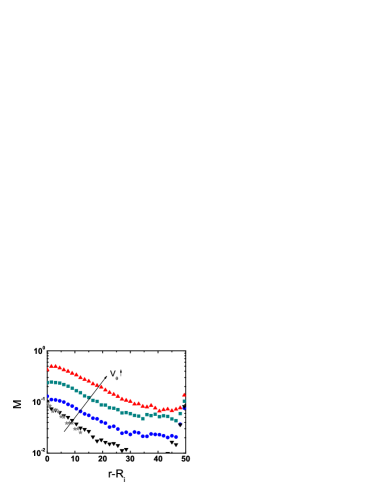
Figure 25: (Color online) Influence of shear velocity $V_{\theta}$ on the mobilization of friction profiles $M(r)$. (${\color[rgb]{0.50,0.50,0.50}\bigstar}$) $V_{\theta}=0,00025$, ($\blacktriangledown$) $V_{\theta}=0.0025$, (${\color[rgb]{0.00,0.00,1.00}\bullet}$) $V_{\theta}=0.025$, (${\color[rgb]{0.25,0.50,0.50}\blacksquare}$) $V_{\theta}=0.25$, (${\color[rgb]{0.98,0.00,0.00}\blacktriangle}$) $V_{\theta}=2.5$. Geometry $R_{50}$.

For any quantity $q(r)$ averaged in space (along $\theta$) and in time, we may define its fluctuation:

$$\delta q(r)^{2} = \frac{1}{\Theta}\int_{0}^{\Theta}q(r,\theta)^{2}d\theta-q(r)^{2},$$ (26)

where $q(r,\theta)^{2}$ is averaged in time. We measure the fluctuations of the translational and rotational velocities $\delta v_{\theta}(r)$, $\delta v_{r}(r)$ and $\delta\omega(r)$. Our analysis (long time scale) takes into account both the small fluctuations around the mean motion (in the cage formed by the nearest neighbors), and the large fluctuations associated to collective motions Radjaï and Roux (2002).

Fig. 26 first shows that the general amplitude of the fluctuations increases with $V_{\theta}$. Then, for various $V_{\theta}$, they reveal a strong decay of the fluctuating quantities close to the inner wall, comparable to that of the respective average quantities, consistently with previous observations Denniston and Li (1999); Schollmann (1999); Veje et al. (1999); Mueth et al. (2000); Mueth (2003); da Cruz et al. (2005). This decay is still true at larger distances for $\delta v_{\theta}$ and $\delta\omega$ (with an increase close to the outer wall). We also notice a stabilization of $\delta v_{r}$, which occurs at $r-R_{i}\approx 10$ for $V_{\theta}=0.025$ and at $r-R_{i}\approx 20$ for $V_{\theta}=2.5$, that is to say precisely when the solid fraction $\nu$ reaches a value $\approx 0.82$ (Fig. 6). Above this critical value of $\nu$, the material would be so compact that the radial motions would take place as a block. Fig. 26a shows the equality of $\delta v_{\theta}$ and $\delta v_{r}$ before the stabilization of $\delta v_{r}(r)$, while Fig. 26b shows the systematic equality of $\delta v_{\theta}$ and $\delta\omega/2$.

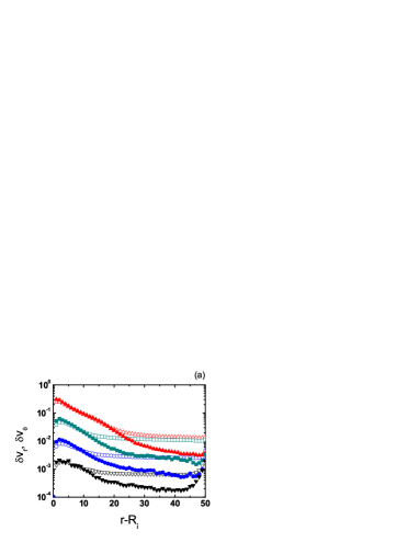
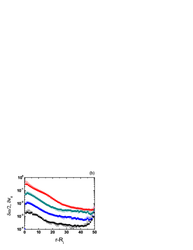
Figure 26: (Color online) (a) Comparison between the profiles of the fluctuations of the radial velocity $\delta v_{r}$ (hollow symbols) and of the orthoradial velocity $\delta v_{\theta}$ (full symbols). (b) Comparison between the profiles of the fluctuations of the angular velocity $\delta\omega/2$ (hollow symbols) and of the orthoradial velocity $\delta v_{\theta}$ (full symbols) for different wall velocities $V_{\theta}$: ($\triangledown$, $\blacktriangledown$) $V_{\theta}=0.0025$, (${\color[rgb]{0.00,0.00,1.00}\circ,\bullet}$) $V_{\theta}=0.025$, (${\color[rgb]{0.25,0.50,0.50}\square,\blacksquare}$) $V_{\theta}=0.25$, (${\color[rgb]{0.98,0.00,0.00}\vartriangle,\blacktriangle}$) $V_{\theta}=2.5$. Geometry $R_{50}$.

References

- Pouliquen and Chevoir (2002) O. Pouliquen and F. Chevoir, Comptes-Rendus Physique 3, 163 (2002).
- GDR MIDI (2004) GDR MIDI, Euro. Phys. J. E 14, 341 (2004).
- Forterre and Pouliquen (2008) Y. Forterre and O. Pouliquen, Annu. Rev. Fluid Mech. 40, 1 (2008).
- da Cruz et al. (2005) F. da Cruz, S. Emam, M. Prochnow, J.-N. Roux, and F. Chevoir, Phys. Rev. E 72, 021309 (2005).
- Lois et al. (2005) G. Lois, A. Lemaître, and J. M. Carlson, Phys. Rev. E 72, 051303 (2005).
- Chevoir et al. (2008) F. Chevoir, J.-N. Roux, F. da Cruz, P. Rognon, and G. Koval, Powder Tech. (2008), doi:10.1016/j.powtec.2008.04.061.
- Jop et al. (2006) P. Jop, Y. Forterre, and O. Pouliquen, Nature 441, 727 (2006).
- Hatano (2007) T. Hatano, Phys. Rev. E 75, 060301 (2007).
- Peyneau and Roux (2008) P.-E. Peyneau and J.-N. Roux, Phys. Rev. E 78, 011307 (2008).
- Goldhirsch (2003) I. Goldhirsch, Annu. Rev. Fluid Mech. 35, 267 (2003).
- Schofield and Wroth (1968) A. N. Schofield and C. P. Wroth, Critical state soil mechanics (McGraw-Hill, London, 1968).
- Wood (1990) D. M. Wood, Soil Behaviour and Critical State Soil Mechanics (Cambridge University Press, 1990).
- de Ryck et al. (2008) A. de Ryck, R. Ansart, and J. A. Dodds, Granular Matter 10, 353 (2008).
- Jop et al. (2005) P. Jop, Y. Forterre, and O. Pouliquen, J. Fluid Mech. 541, 167 (2005).
- Miller et al. (1996) B. Miller, C. O’Hern, and R. P. Behringer, Phys. Rev. Lett. 77, 3110 (1996).
- Elliott et al. (1998) K. E. Elliott, G. Ahmadi, and W. Kvasnak, J. Non Newtonian Fluid Mech. 74, 89 (1998).
- Veje et al. (1999) C. Veje, D. Howell, and R. Behringer, Phys. Rev. E 59, 739 (1999).
- Howell et al. (1999a) D. Howell, R. Behringer, and C. Veje, Phys. Rev. Lett. 82, 5241 (1999a).
- Hartley and Behringer (2003) R. Hartley and R. Behringer, Nature 421, 928 (2003).
- Tardos et al. (1998) G. Tardos, M. Khan, and D. Schaeffer, Phys. Fluids 10, 335 (1998).
- Howell et al. (1999b) D. Howell, R. Behringer, and C. Veje, Chaos 9, 559 (1999b).
- Mueth et al. (2000) D. Mueth, G. Debregeas, G. Karczmar, P. Eng, S. Nagel, and H. Jaeger, Nature 406, 385 (2000).
- Klausner et al. (2000) J. Klausner, D. Chen, and R. Mei, Powder Tech. 112, 94 (2000).
- Cain (2001) R. Cain, Phys. Rev. E 64, 016413 (2001).
- Losert and Kwon (2001) W. Losert and G. Kwon, Advances in Complex Systems 4, 369 (2001).
- Bocquet et al. (2002) L. Bocquet, W. Losert, D. Schalk, T. C. Lubensky, and J. P. Gollub, Phys. Rev. E 65, 011307 (2002).
- da Cruz et al. (2002) F. da Cruz, F. Chevoir, D. Bonn, and P. Coussot, Phys. Rev. E 66, 051305 (2002).
- Mueth (2003) D. Mueth, Phys. Rev. E 67, 011304 (2003).
- Chambon et al. (2003) G. Chambon, J. Schmittbuhl, A. Corfdir, J.-P. Vilotte, and S. Roux, Phys. Rev. E 68, 011304 (2003).
- Tardos et al. (2003) G. Tardos, S. McNamara, and I. Talu, Powder Tech. 131, 23 (2003).
- Utter and Behringer (2004) B. Utter and R. P. Behringer, Euro. Phys. J. E 14, 373 (2004).
- da Cruz (2004) F. da Cruz, Ph.D. thesis, Ecole Nationale des Ponts et Chaussées (2004), in French (http://pastel.paristech.org/946).
- Daniel et al. (2007) R. Daniel, A. Poloski, and A. Saez, Powder Tech. 179, 62 (2007).
- Wang et al. (2008) P. Wang, C. Song, C. Briscoe, and H. Makse, Phys. Rev. E 77, 061309 (2008).
- Nedderman (1992) R. Nedderman, Statics and kinematics of granular materials (Cambridge University Press, Cambridge, 1992).
- Savage (1989) S. B. Savage, in Theoretical and applied mechanics, edited by M. Piau and D. Caillerie (North Holland, Amsterdam, 1989), pp. 241–266.
- Chambon et al. (2006) G. Chambon, J. Schmittbuhl, and A. Corfdir, J. Geophys. Res. 111, B09309 (2006).
- Karion and Hunt (1999) A. Karion and M. Hunt, Journal of Heat Transfer 121, 984 (1999).
- Schollmann (1999) S. Schollmann, Phys. Rev. E 59, 889 (1999).
- Lätzel et al. (2000) M. Lätzel, S. Luding, and H. J. Hermann, Granular Matter 2, 123 (2000).
- Zervos et al. (2000) A. Zervos, I. Vardoulakis, M. Jean, and P. Lerat, Mech. Cohes. Frict. Mat. 5, 305 (2000).
- Koval (2008) G. Koval, Ph.D. thesis, Ecole Nationale des Ponts et Chaussées (2008), in French, http://tel.archives-ouvertes.fr/tel-00311984/fr/.
- Corfdir et al. (2004) A. Corfdir, P. Lerat, and I. Vardoulakis, Geotechnical Testing Journal 27, 447 (2004).
- Lätzel (2003) M. Lätzel, Ph.D. thesis, University of Stuttgart (2003).
- Cundall and Strack (1979) P. A. Cundall and O. D. L. Strack, Géotech. 29, 47 (1979).
- Silbert et al. (2001) L. E. Silbert, D. Ertas, G. S. Grest, T. Halsey, D. Levine, and S. J. Plimpton, Phys. Rev. E 64, 385 (2001).
- Roux and Chevoir (2005) J. N. Roux and F. Chevoir, Bulletin des Laboratoires des Ponts et Chaussées 254, 109 (2005).
- Rognon et al. (2008) P. Rognon, J. N. Roux, M. Naaïm, and F. Chevoir, J. Fluid Mech. 596, 21 (2008).
- Allen and Tildesley (1987) M. P. Allen and D. J. Tildesley, Computer simulation of liquids (Oxford University Press, Oxford, 1987).
- Cui et al. (2007) L. Cui, C. O’Sullivan, and S. O’Neill, Géotech. 57, 831– (2007).
- Campbell (2002) C. S. Campbell, J. Fluid Mech. 465, 261 (2002).
- Combe (2002) G. Combe, Microscopic origins of strain in granular materials, vol. SI8 (Collection Etudes et Recherches des Laboratoires des Ponts et Chaussées, Paris, 2002), in French (http://pastel.paristech.org/51/).
- Radjaï and Roux (2004) F. Radjaï and S. Roux, in The physics of granular media, edited by H. Hinrichsen and D. Wolf (Wiley-Vch, Weinheim, 2004), pp. 165–187.
- Radjaï (2008) F. Radjaï (2008), arXiv:0801.4722.
- Coleman et al. (1966) B. Coleman, H. Markovitz, and W. Noll, Viscosimetric flows of non Newtonian fluids (Springer-Verlag, Berlin, 1966).
- Savage and Sayed (1984) S. B. Savage and M. Sayed, J. Fluid Mech. 142, 391 (1984).
- Losert et al. (2000) W. Losert, L. Bocquet, T. C. Lubensky, and J. Gollub, Phys. Rev. Lett. 85, 1428 (2000).
- Denniston and Li (1999) C. Denniston and H. Li, Phys. Rev. E 59, 3289 (1999).
- Ertas et al. (2001) D. Ertas, G. S. Grest, T. C. Halsey, D. Levine, and L. Silbert, Europhys. Lett. 56, 214 (2001).
- Chevoir et al. (2001) F. Chevoir, M. Prochnow, J. Jenkins, and P. Mills, in Powders and grains 2001, edited by Y. Kishino (Balkema, Rotterdam, 2001), pp. 373–376.
- Mills et al. (2008) P. Mills, P. Rognon, and F. Chevoir, Europhys. Lett. 81, 64005 (2008).
- Tejchman and Wu (1993) J. Tejchman and W. Wu, Acta Mechanica 99, 61 (1993).
- Mohan et al. (2002) L. S. Mohan, K. K. Rao, and P. R. Nott, J. Fluid Mech. 457, 377 (2002).
- Artoni et al. (2008) R. Artoni, P. Canu, and A. Santomaso (2008), arXiv:0803.3890.
- Rajchenbach (2000) J. Rajchenbach, Adv. in Physics 49, 229 (2000).
- Khakhar et al. (2001) D. Khakhar, A. Orpe, P. Andresen, and J. Ottino, J. Fluid Mech. 441, 255 (2001).
- Komatsu et al. (2001) T. S. Komatsu, S. Inagaki, M. Nakagawa, and S. Nasuno, Phys. Rev. Lett. 86, 1757 (2001).
- Crassous et al. (2008) J. Crassous, J.-F. Metayer, P. Richard, and C. Laroche, J. Stat. Mech. (2008), doi: 10.1088/1742-5468/2008/03/P03009.
- Debrégeas and Josserand (2000) G. Debrégeas and C. Josserand, Europhys. Lett. 52, 137 (2000).
- Lagree and Lhuillier (2006) P.-Y. Lagree and D. Lhuillier, Eur. J. Mech. B 25, 960 (2006).
- Falk et al. (2008) M. L. Falk, M. Toiya, and W. Losert (2008), arXiv:0802.1752.
- Debrégeas et al. (2001) G. Debrégeas, H. Tabuteau, and J.-M. di Meglio, Phys. Rev. Lett. 87, 178305 (2001).
- Huang et al. (2005) N. Huang, G. Ovarlez, F. Bertrand, S. Rodts, P. Coussot, and D. Bonn, Phys. Rev. Lett. 94, 028301 (2005).
- Moreau (1997) J.-J. Moreau, in Friction, Arching, Contact Dynamics, edited by D. E. Wolf and P. Grassberger (World Scientific, Londres, 1997), pp. 233–247.
- Staron et al. (2002) L. Staron, J.-P. Vilotte, and F. Radjaï, Phys. Rev. Lett. 89, 204302 (2002).
- Radjaï and Roux (2002) F. Radjaï and S. Roux, Phys. Rev. Lett. 89, 064302 (2002).