The Sensing Capacity of Sensor Networks

Abstract

This paper demonstrates fundamental limits of sensor networks for detection problems where the number of hypotheses is exponentially large. Such problems characterize many important applications including detection and classification of targets in a geographical area using a network of sensors, and detecting complex substances with a chemical sensor array. We refer to such applications as large-scale detection problems. Using the insight that these problems share fundamental similarities with the problem of communicating over a noisy channel, we define a quantity called the ‘sensing capacity’ and lower bound it for a number of sensor network models. The sensing capacity expression differs significantly from the channel capacity due to the fact that a fixed sensor configuration encodes all states of the environment. As a result, codewords are dependent and non-identically distributed. The sensing capacity provides a bound on the minimal number of sensors required to detect the state of an environment to within a desired accuracy. The results differ significantly from classical detection theory, and provide an intriguing connection between sensor networks and communications. In addition, we discuss the insight that sensing capacity provides for the problem of sensor selection.

I Introduction

A  sensor network is deployed to obtain information about the state of an environment using multiple sensors. In many sensing applications, such as pollution monitoring and border security, the phenomena under observation has a large scale that exceeds the range of any one sensor. As a result, collecting measurements from multiple sensors is essential to the sensing task. Obtaining information about an environment can be cast as either a ‘detection’ or an ‘estimation’ problem. In estimation problems such as the problem of estimating a continuous field to within a desired distortion, the state of the environment is continuous. In detection problems, such as binary hypothesis testing, the state of the environment is represented as a finite set of hypotheses. In this paper we study the problem of ‘large-scale detection’ where the state of the environment belongs to an exponentially large, structured set of hypotheses. Large-scale detection problems include many applications where a sensor network is deployed in order to monitor a large-scale phenomena. We exploit the structure of large-scale detection problems to demonstrate a fundamental information-theoretic relationship between the number of sensor measurements and ability of a sensor network to detect the state of the environment to within a desired accuracy.

We obtain our results by drawing on an analogy between sensor networks and channel encoders. For a fixed sensor configuration, each state of the environment induces a corresponding set of sensor outputs. This set of sensor outputs can be viewed as a noise-corrupted ‘codeword,’ which must be ‘decoded’ in order to detect the state of the environment. Thus, the sensor network acts as a channel encoder. In order to motivate this perspective, we examine the following large-scale detection applications.

Robotic mapping is the first large-scale application we consider [1]. In mapping, robots collect sensor measurements to map an unknown environment for the purpose of navigation. [2] introduced occupancy grids, one of the most popular approaches to this problem. In occupancy grids, the world is modeled as a discrete grid, where each grid location has a value corresponding to the state of the environment. For example, in a binary a grid a ‘0’ can indicate free space while a ‘1’ can indicate an obstacle. A robot traversing an unknown environment collects sensor measurements that encode the state of the environment. For example, a robot using a sonar sensor emits a wide acoustic pulse and measures the time until a reflected pulse is sensed. These readings are ambiguous, since one cannot infer the precise location of the obstacle that caused the reflection from a single sensor reading. In addition, sonar readings are noisy. As a result, multiple sensor measurements must be used to distinguish among an exponentially large number of possible grid states. The sequence of sonar readings can be viewed as a noise-corrupted codeword corresponding to the state of the grid. While robotic mapping systems have been successfully implemented in practice, little can be said about their theoretical performance. Theoretical understanding could shed light on the number of sensor measurements required to map an unknown environment. In addition, theory can provide insight into questions about sensor selection. Is it better to use cheap, low power, wide angle sensors or expensive, high power, narrow angle sensors? A theoretical framework could provide general insight into such sensor selection questions.

Video surveillance is another large scale detection problem. [3] used multi-camera sensor networks to detect and track objects across multiple areas, and [4] uses multiple cameras to localize moving objects in a room. The region under surveillance can be viewed as a three-dimensional grid. For example each grid position can have a binary value, representing motion or lack of motion in that grid position. As in the previous example, the number of states of this grid is exponential in the number of grid blocks. Each camera observes a subset of grid blocks, but introduces ambiguity by reducing a three-dimensional volume to a two-dimensional image. As a result multiple camera images must be combined to detect the state of the environment. The set of images encode the grid state. While practical systems for surveillance applications are deployed, a theoretical framework for understanding performance limits for such problems is not available.

Identifying a complex chemical substance is a third example of a large-scale detection problem. In this application the output of chemical sensor arrays, consisting of heterogeneous chemical sensors, is used to distinguish among a large number of substances [5]. Each substance can be modeled as a mixture of constituent chemicals at various discrete concentration levels, resulting in an exponentially large set of possible states. Each chemical sensor in the array reacts to a subset of chemicals. For example, sensors can output a voltage proportional to a weighted sum of the concentrations of a subset of chemicals. The output of a chemical sensor array encodes the state of the sample being sensed. As in the previous two examples, theory could provide insight into the practical design of such sensor arrays.

Target detection and classification in a geographical area is an important class of applications for sensor networks [6], and a final motivating example of a large-scale detection problem. We consider the problem of detection and classification using seismic sensors, as demonstrated in [6],[7]. The environment can be modeled as a discrete grid, where each position can contain targets of multiple types. The number of target configurations is exponential in the number of grid blocks. Seismic sensors are scattered randomly on this grid, and sense the vibrations of targets over subsets of the grid. The intensity of vibration is dependent on the target’s distance from the sensor, and therefore a single sensor cannot distinguish between many targets far away and a single target nearby. The set of seismic sensor outputs encode the location and class of targets in the field.

All of the examples considered above share the following common elements. The state can be modeled as a discrete vector or grid, and the number of states is exponentially large. Sensors output noise-corrupted functions of subsets of the vector or grid. These sensor measurements must be fused in order to detect the state of the environment. In this paper we analyze the fundamental limits of this process by using the insight that the problem of large-scale detection and the problem of communicating over a noisy channel share essential similarities.

II Sensor Networks and Communication Channels

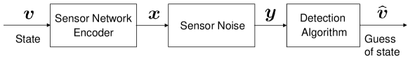
Figure 1: Sensor network model.

The examples described in Section I motivate the sensor network model shown in Figure 1. A discrete target vector $\boldsymbol{v}$ represents the state of the environment. In this paper, the term ‘state’ and ‘target vector’ are used interchangeably. A fixed sensor configuration encodes the state as a vector of noiseless sensor outputs that form the codeword $\boldsymbol{x}$. The observed, noisy sensor measurements are written as $\boldsymbol{y}$, a noise-corrupted version of $\boldsymbol{x}$. Finally, a detection algorithm uses $\boldsymbol{y}$ to compute a guess of the state of the environment $\hat{\boldsymbol{v}}$.

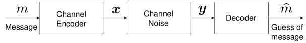
Figure 2: Communication channel model.

The sensor model shown in Figure 1 is similar to the classical communication channel model shown in Figure 2. The target vector $\boldsymbol{v}$ corresponds to the message $m$ being sent. The sensor network acts as a channel encoder, producing the codeword $\boldsymbol{x}$. Finally, a detection algorithm acts as a channel decoder on the noise corrupted codeword $\boldsymbol{y}$. Shannon’s celebrated Channel capacity results provide limits for the communications channel [8]. Motivated by the similarity between the sensor network model and the communication channel model, we defined and bounded the sensing capacity in [9]. The sensing capacity plays a role in our sensor network model analogous to the role of channel capacity in a communications channel. However, because the models differ in significant ways, the notions of channel capacity and sensing capacity also differ.

The most important difference between the sensor network model and a communication channel model is at the encoder. In communications, the content of the message and its codeword representation can be decoupled. Further, the channel encoder can implement any mapping between message and codeword. As a result, two highly similar messages can be differentiated with arbitrarily high accuracy. In contrast, a sensor network encoder uses the same sensor configuration to encode all states of the environment. Further, since sensors react to some phenomena in the environment and are limited by physical constraints, the codeword associated with a particular state of the environment is a direct function of that state. Therefore the state and its codeword representation are coupled. As a result, two highly similar states of the environment cannot be distinguished with arbitrarily high accuracy. While similarities between the sensor network model and the channel model motivate the application of insights about communications from information theory, significant differences between the two models require care in applying such insights in order to understand the impact of these differences on the final theoretical results.

Section III provides an overview of the main results presented in this paper, and reviews related work. Section IV presents sensing capacity results for non-spatial (e.g. chemical) sensing applications, while Section V demonstrates sensing capacity results for a sensor network model that accounts for spatial locality in sensor observations. Section VI concludes the paper and discusses future work.

III Main Results and Related Work

We review the main theoretical results presented in this paper. In Section IV we introduce a simple but useful sensor network model that can be used to model sensing applications such as chemical sensing applications and computer network monitoring. For this model, we define and bound the sensing capacity. The sensing capacity bound differs significantly from the standard channel capacity results, and requires novel arguments to account for the constrained encoding of a sensor network. This is an important observation due to the use of mutual information as a sensor selection heuristic [10]. Our result shows that this is not the correct metric for large-scale detection applications. Extensions are presented to account for non-binary target vectors, target sparsity, and heterogeneous sensors. Plotting the sensing capacity bound, we demonstrate interesting sensing tradeoffs. For example, perhaps counter-intuitively, sensors of shorter range can achieve a desired detection accuracy with fewer measurements than sensors of longer range. Finally, we also compare our sensing capacity bound to simulated sensor network performance.

In Section V we introduce a sensor network model that accounts for contiguity in a sensor’s field of view. Contiguity is an essential aspect of many classes of sensors. For example, cameras observe localized regions and seismic sensors sense vibrations from nearby targets. We demonstrate sensing capacity bounds that account for such sensors by extending results about Markov types [11], and use convex optimization to compute these bounds. The first result in Section V assumes the state of the environment is modeled as a one-dimensional vector. In Section V-D we extend this result to the case where the state of the environment is modeled as a two-dimensional grid. While a one-dimensional vector can model sensor network applications such as border security and traffic monitoring, results about two dimensions significantly increase the type of applications described by our models.

The performance of sensor networks is limited by both sensing resources and non-sensing resources such as communications, computation, and power. One set of results has been obtained by considering the limitations that communications requirements impose on a sensor network. [12] extends the results in [13] to account for the different traffic models that arise in a sensor network. [14] studies network transport capacity for the case of regular sensor networks. [15] studies the impact of computational constraints and power on the communication efficiency of sensor networks. [16] has considered the interaction between transmission rates and power constraints. Another set of results has been obtained by extending results from compression to sensor networks. Distributed source coding [17],[18] provides limits on the compression of separately encoded correlated sources. [19] applies these results to sensor networks. [20] provides an overview of this area of research.

In contrast to the work mentioned above, we focus directly on the limits of detecting the state of the environment using noisy sensor observations. The notion of sensing capacity characterizes the limits that sensing (e.g. sensor type, range, and noise) imposes on the attainable accuracy of detection. We do not examine the compression of sensor observations, or the resources required to communicate sensor observations to a point in the network. Instead, we focus on the limits of detection accuracy assuming complete availability of noisy sensor observations. Among existing work in information theory, the problem we investigate in this paper is unlike a source coding problem, and is similar to a channel coding problem. However, the sensor network model we investigate is fundamentally different than a standard communications channel.

Our work is most closely related to work on detection and classification in sensor networks. [21] describes a large body of work on distributed detection where the number of hypotheses is small. [22], [23] extend this work to consider a decentralized binary detection problem with noisy communication links to obtain error exponents. [24] analyzes the performance of various classification schemes for classifying a Gaussian source. This is an m-ary problem where the number of hypotheses is small. [25] analyzes the performance suboptimal classification schemes for classifying multiple targets. While the number of hypotheses is exponential in the number of targets, the large-scale detection problem of a large number of targets is not considered. [26] considers the problem of sensor placement for detecting the location of one or few targets in a grid. This problem is most closely related to the large-scale detection problems addressed in this paper. However, due to restrictions on the numbers of targets, the number of hypotheses remains small in comparison to a large-scale detection problem. A coding-based approach was used to bound the minimum number of sensors required for discrimination, and to propose structured sensor configurations. However, sensors were noiseless, and of limited type, and no notion of sensing capacity was considered. In contrast to existing to existing work on detection and classification in sensor networks, we demonstrate fundamental performance limits for large-scale detection problems.

The problem of estimating a continuous field using a sensor network is an active area of research. [27] considers the relationship of transport capacity and the rate distortion function of a continuous random processes. [28] proves limits on the estimation of an inhomogeneous random fields using sensor that collect noisy point samples. Other work on the problem of estimating a continuous random field includes [29],[30], [31],[32]. [33] considers the estimation of continuous parameters of a set of underlying random processes through a noisy communications channel. The results presented in this paper consider the detection of a discrete state of an environment. We do not consider extensions to environments with a continuous state.

IV Sensing Capacity of the Arbitrary Connections Model

In this section we define and analyze the sensing capacity of the arbitrary connections model, a simple but useful model introduced in [9]. We denote random variables and functions by upper-case letters, and instantiations or constants by lower-case letters. Bold-font denotes vectors. $\log(\cdot)$ has base-2. Sets are denoted using calligraphic script. $D(P||Q)$ denotes the Kullback-Leibler distance and $H(P)$ denotes entropy of a random variable with probability distribution $P$. $H(Q|P)$ is the conditional entropy of a random variable with conditional probability distribution $Q$ given another random variable with probability distribution $P$.

IV-A Arbitrary Connections Model

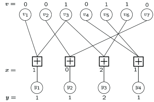
Figure 3: Arbitrary connections model with $k=7,n=4,c=2,$ and a sum sensing function.

Figure 3 shows an example of the arbitrary connections model. The state of the environment is modeled as a $k$-dimensional binary target vector $\boldsymbol{v}$. Each position in the vector may represent the presence of a target in an actual region in space, or may have other interpretations, such as the presence of a specific chemical in a sample. The possible target vectors are denoted $\boldsymbol{v_{i}}$, $i\in\{1,\ldots,2^{k}\}$. We say that ‘a certain $\boldsymbol{v}$ has occurred’ if that vector represents the true state. We define a sensor network $s(k,n)$ as a graph showing the connections of $n$ sensors to $k$ positions in the target vector. The sensor network has $n$ identical sensors. Sensor $\ell$ senses exactly $c$ out of the $k$ spatial positions (shown in the graph as $c$ connections). We refer to such sensors as having a range $c$. Ideally, each sensor produces a value $x\in{\cal X}$ that is an arbitrary function of the targets which it senses, $x_{\ell}=\Psi(v_{\ell t_{1}},\ldots,v_{\ell t_{c}})$. Thus, the ‘ideal output vector’ of the sensor network $\boldsymbol{x}$ depends on the sensor connections, and on the target vector $\boldsymbol{v}$ that occurs. However, we assume that each sensor output $y\in\mathcal{Y}$ is corrupted by noise, so that the conditional p.m.f. $P_{Y|X}(y|x)$ determines the output. Since the sensors are identical, $P_{Y|X}$ is the same for all the sensors. Further, we assume that the noise is independent in the sensors, so that the ‘sensor output vector’ $\boldsymbol{y}$ relates to the ideal output $\boldsymbol{x}$ as $P_{\boldsymbol{Y}|\boldsymbol{X}}(\boldsymbol{y}|\boldsymbol{x})=\prod_{\ell=1}^{n}P_{Y|X}(y_{\ell}|x_{\ell})$. Given the noise corrupted output $\boldsymbol{y}$ of the sensor network, we detect the target vector $\boldsymbol{v}$ which occurred by using a detector $g(\boldsymbol{y})$. Because of the constrained encoding of a sensor network, we allow the decoder a distortion of $D\in[0,1]$. Denoting $d_{\text{H}}(\boldsymbol{v_{i}},\boldsymbol{v_{j}})$ as the Hamming distance between two target vectors, the tolerable distortion region of $\boldsymbol{v_{i}}$ is $\mathcal{D}_{\boldsymbol{v_{i}}}=\{j:\frac{1}{k}d_{\text{H}}(\boldsymbol{v_{i}},\boldsymbol{v_{j}})<D\}$. Given that $\boldsymbol{v_{i}}$ occurred, the detector is in error if $g(\boldsymbol{y})\not\in\mathcal{D}_{\boldsymbol{v_{i}}}$.

Figure 3 shows the target vector $\boldsymbol{v}=(0,0,1,0,1,1,0)$ indicating $3$ targets among the $7$ target positions. In this example, the sensing function $\Psi$ is a sum that indicates the number of positions which contain a target, $x_{\ell}=\sum_{u=1}^{c}v_{\ell t_{u}}$, so that $x\in{\cal X}=\{0,1,\ldots,c\}$. Such a function could model a chemical sensor that is sensitive to a subset of chemicals and whose output is linearly proportional to the number of such chemicals present in the sample. More complex, e.g. nonlinear, relationships between chemicals and sensor output require a different choice of $\Psi$. In the figure,each sensor senses two target positions, and the sensors encode the target vector as $\boldsymbol{x}=(1,0,2,1)$. However, due to noise, the observed vector of sensor outputs is $\boldsymbol{y}=(1,1,2,1)$. The target vector $\boldsymbol{v}^{\prime}=(0,1,1,0,1,1,0)$, which differs from $\boldsymbol{v}$ in one target position, is encoded as $\boldsymbol{x}=(1,1,2,1)$. As a result a detection algorithm can easily confuse $\boldsymbol{v}^{\prime}$ for $\boldsymbol{v}$, demonstrating the limitation imposed by the constrained encoding of a sensor network.

The arbitrary connections model describes large-scale detection problems that do not have a spatial aspect. Examples of such applications include the detection of complex chemical and computer network monitoring. Disease detection in a population where individual sample can be combined is another such application. In addition to practical utility, this model is easy to analyze and provides useful insights into large-scale detection problems.

IV-B Sensing Capacity Definitions

How many sensor measurements must a sensor network collect to detect the a target vector to within a desired distortion? To answer this question we define the idea of a ‘sensing capacity.’ The probability of error of a sensor network given a that target vector $\boldsymbol{v_{i}}$ occurred is $P_{e,i,s}=\text{Pr}(\text{error}|i,s,\boldsymbol{x_{i}},\boldsymbol{y})=\text{Pr}(g(\boldsymbol{y})\not\in\mathcal{D}_{\boldsymbol{v_{i}}}|\boldsymbol{v_{i}},s,\boldsymbol{x_{i}},\boldsymbol{y})$. The expected probability of error for a sensor network is $P_{e,s}=\sum_{i}P_{e,i,s}P_{\boldsymbol{V}}(\boldsymbol{v_{i}})$. The rate $R$ of a sensor network is defined as the ratio of target positions being sensed to the number of sensor measurements, $R=\frac{k}{n}$. The sensing capacity of a sensor network, $C(D)$, is defined as the maximum rate $R$ such that below this rate there exists a sequence of sensor networks $s(\lceil nR\rceil,n)$ whose expected probability of error across all target vector goes to zero with increasing $n$, that is, $P_{e,s}\rightarrow 0$ as $n\rightarrow\infty$ at a fixed rate $R$.

Is $C(D)$ nonzero? One of the main contributions of the theorem presented in this section is to demonstrate that the sensing capacity can be strictly positive for the arbitrary connections model. We use a random coding argument to obtain a bound on the sensing capacity for the arbitrary connections model. Instead of constructing a sequence of sensor network directly, we bound the expected probability of error, averaged over a randomly generated ensemble of sensor networks. The sensor networks are generated as follows. Each sensor connects to $c$ randomly chosen target positions out of the $k$ possible positions. The connections are made independently, and are chosen with replacement. Therefore a sensor can choose the same target position more than once. When we take the expectation over all such randomly generated sensor networks, the ideal sensor outputs associated with each target vector become random. Since a sensor network produces a codeword that is a function of the target vector, codeword distribution depends on the occurring target vector. We denote the random vector which occurs when $\boldsymbol{v_{i}}$ is the target vector as $\boldsymbol{X_{i}}$. Because each sensor forms its connections independently,$P_{\boldsymbol{X_{i}}}(\boldsymbol{x_{i}})=\prod_{\ell=1}^{n}P_{X_{i}}(x_{i\ell})$. It is important to note that sensor outputs are in general not independent, and are only independent when we condition on the occurrence of a particular target vector. Further, it is important to note that the random vectors $\boldsymbol{X_{i}}$ and $\boldsymbol{X_{j}}$, associated with a pair of target vectors, $\boldsymbol{v_{i}}$ and $\boldsymbol{v_{j}}$ respectively, are not independent, since the sensor connections produce a dependency between them. Thus, the ‘codewords’ $\{\boldsymbol{X_{i}},i=1,2,\ldots,2^{k}\}$ of the sensor network are non-identical and dependent on each other, unlike channel codes in classical information theory. Using this probabilistic model for sensor network generation, we write the expected probability of error, averaged over the sensor network ensemble as $P_{e}={\rm E}\,_{S}[P_{e,S}]$. Theorem 1 in Section IV-C bounds this quantity to prove a lower bound $C_{LB}(D)$ on the sensing capacity $C(D)$.

The statement of the result presented in this section relies on the method of types [11], and requires an explanation of types and joint types. Since in the random sensor network construction each sensor connects to $c$ target positions independently, the distribution of a sensor’s ideal output $X_{i}$ depends only on the type $\boldsymbol{\gamma}=(\gamma_{0},\gamma_{1})$ of $\boldsymbol{v_{i}}$. The type of target vector $\boldsymbol{v_{i}}$ is a histogram of the number of 0’s and 1’s in $\boldsymbol{v_{i}}$. Here, $\gamma_{0}$ denotes the fraction of zeros in $\boldsymbol{v_{i}}$. Since sensor connections are generated independently and uniformly across target positions in the arbitrary connections model we can write, $P_{\boldsymbol{X_{i}}}(\boldsymbol{x_{i}})=P^{\boldsymbol{\gamma},n}(\boldsymbol{x_{i}})=\prod_{\ell=1}^{n}P^{\boldsymbol{\gamma}}(x_{i\ell})$ for all $\boldsymbol{v_{i}}$ of the same type $\boldsymbol{\gamma}$.

Since a single sensor network encodes all target vectors, pairs of codewords are dependent, unlike codes in communications. The joint probability of two codewords $P_{\boldsymbol{X_{i}}\boldsymbol{X_{j}}}$ depends on the joint type of the target vectors $\boldsymbol{v_{i}}$ and $\boldsymbol{v_{j}}$. The joint type is $\boldsymbol{\lambda}=(\lambda_{00},\lambda_{01},\lambda_{10},\lambda_{11})$. Here, $\lambda_{01}$ is the fraction of positions in $\boldsymbol{v_{i}},\boldsymbol{v_{j}}$ where $\boldsymbol{v_{i}}$ has bit ‘0’ while $\boldsymbol{v_{j}}$ has bit ‘1’. Similarly, we define $\lambda_{00},\lambda_{10},\lambda_{11}$.

Following the notation introduced in [11], $\boldsymbol{\lambda}\ \in\ {\mathcal{P}}_{k}(\{0,1\}^{2})$, indicating that $\boldsymbol{\lambda}$ is in the set of joint types of $k$-bit binary vector pairs. Again, since sensor connections are generated independently and with uniform probability across target positions, $P_{\boldsymbol{X_{i}},\boldsymbol{X_{j}}}(\boldsymbol{x_{i}},\boldsymbol{x_{j}})=P^{\boldsymbol{\lambda},n}(\boldsymbol{x_{i}},\boldsymbol{x_{j}})=\prod_{\ell=1}^{n}P^{\boldsymbol{\lambda}}(x_{i\ell},x_{j\ell})$ for all $\boldsymbol{v_{i}},\boldsymbol{v_{j}}$ of the same joint type $\boldsymbol{\lambda}$. Since the joint type $\boldsymbol{\lambda}$ also defines the type $\boldsymbol{\gamma}$ of $\boldsymbol{v_{i}}$, we have $\lambda_{00}+\lambda_{01}=\gamma_{0}$, $\lambda_{10}+\lambda_{11}=\gamma_{1}$.

We give specific examples of these quantities using the example shown in Figure 3 where $c=2$ and sensors count the number of targets present in the target positions that they sense. Table I lists the types of four vectors $\boldsymbol{v_{j}}$, and their joint type with the target vector in the example $\boldsymbol{v_{i}}=0010110$. Given a target vector, a sensor will output ‘2’ only if both of its connections connect to positions with a ‘1.’ For a vector of type $\boldsymbol{\gamma}$, this occurs with probability $(\boldsymbol{\gamma}_{1})^{2}$. Table II describes the complete output p.m.f. for a randomly generated sensor, given that a vector of type $\boldsymbol{\gamma}$ occurred. Given two target vectors $\boldsymbol{v_{i}},\boldsymbol{v_{j}}$ of joint type $\boldsymbol{\lambda}$, a sensor will output ‘0’ for both target vectors only if both its connections are connected to target positions that have a ‘0’ bit in both these target vectors. This happens with probability $(\lambda_{00})^{2}$. Table III lists the complete joint p.m.f. $P_{X_{i}X_{j}}(x_{i},x_{j})=P^{\boldsymbol{\lambda}}(x_{i},x_{j})$ of a randomly generated sensor for two target vectors with a joint type $\boldsymbol{\lambda}$.

IV-C Sensing Capacity Lower Bound

We specify two probability distributions which we will utilize in the main theorem of this section. The first is the joint distribution of the ideal output $\boldsymbol{x_{i}}$ when $\boldsymbol{v_{i}}$ occurs, and the noise corrupted output $\boldsymbol{y}$, $P_{\boldsymbol{X_{i}}\boldsymbol{Y}}(\boldsymbol{x_{i}},\boldsymbol{y})=\prod_{\ell=1}^{n}P_{X_{i}Y}(x_{i\ell},y_{\ell})=\prod_{\ell=1}^{n}P_{X_{i}}(x_{i\ell})P_{Y|X}(y_{\ell}|x_{i\ell})$. The second distribution is the joint distribution of the ideal output $\boldsymbol{x_{i}}$ corresponding to $\boldsymbol{v_{i}}$ and the noise corrupted output $\boldsymbol{y}$ generated by the occurrence of a different target vector $\boldsymbol{v_{j}}$. We can write this joint distribution as $Q_{\boldsymbol{X_{i}}\boldsymbol{Y}}^{(j)}(\boldsymbol{x_{i}},\boldsymbol{y})=\prod_{\ell=1}^{n}Q_{X_{i}Y}^{(j)}(x_{i\ell},y_{\ell})=\prod_{\ell=1}^{n}\sum_{a\in{\mathcal{X}}}P_{X_{i},X_{j}}(x_{i\ell},x_{j}=a)P_{Y|X}(y_{\ell}|x_{j}=a)$. Note that although $\boldsymbol{Y}$ was produced by $\boldsymbol{X_{j}}$, $\boldsymbol{X_{i}}$ and $\boldsymbol{Y}$ are dependent because of the dependence of $\boldsymbol{X_{i}}$ and $\boldsymbol{X_{j}}$.

We argued earlier that due to the random sensor network construction, $P_{\boldsymbol{X_{i}}}$ and $P_{\boldsymbol{X_{i}}\boldsymbol{X_{j}}}$ can be compute using the type $\boldsymbol{\gamma}$ of $\boldsymbol{v_{i}}$ and joint type $\boldsymbol{\lambda}$ of $\boldsymbol{v_{i}},\boldsymbol{v_{j}}$ respectively. Thus, we write $P_{\boldsymbol{X_{i}}\boldsymbol{Y}}(\boldsymbol{x_{i}},\boldsymbol{y})=\prod_{\ell=1}^{n}P_{{X_{i}Y}}^{\boldsymbol{\gamma}}(x_{i\ell},y_{\ell})$ where $P_{{X_{i}Y}}^{\boldsymbol{\gamma}}(x_{i},y)=P^{\boldsymbol{\gamma}}(x_{i})P_{Y|X}(y|x_{i})$. Similarly, we write $Q_{\boldsymbol{X_{i}}\boldsymbol{Y}}^{(j)}(\boldsymbol{x_{i}},\boldsymbol{y})=\prod_{\ell=1}^{n}Q_{{X_{i}Y}}^{\boldsymbol{\lambda}}(x_{i\ell},y_{\ell})$ where $Q_{{X_{i}Y}}^{\boldsymbol{\lambda}}(x_{i},y)=\sum_{a\in{\mathcal{X}}}P^{\boldsymbol{\lambda}}(x_{i},x_{j}=a)P_{Y|X}(y|x_{j}=a)$. We can now ready to state the main theorem of this section.

Theorem 1 (Sensing Capacity Theorem for the Arbitrary Connections Model)

The sensing capacity at distortion $D$ is bounded as,

$$C(D)\geq C_{LB}(D)=\min_{\begin{subarray}{c}\boldsymbol{\lambda}\\ \lambda_{01}+\lambda_{10}\geq D\\ \lambda_{00}+\lambda_{01}=\gamma_{0}\\ \lambda_{10}+\lambda_{11}=\gamma_{1}\end{subarray}}\frac{D\left(P_{X_{i}Y}^{\boldsymbol{\gamma}}\|Q_{{X_{i}Y}}^{\boldsymbol{\lambda}}\right)}{H(\boldsymbol{\lambda})-H(\boldsymbol{\gamma})}$$ (1)

where $\boldsymbol{\gamma}=(0.5,0.5)$ and $\boldsymbol{\lambda}=(\lambda_{00},\lambda_{01},\lambda_{10},\lambda_{11})$ is an arbitrary probability mass functions.

The most striking difference between the result shown in Theorem 1, and Shannon’s channel capacity results is that the bound on the sensing capacity is not a mutual information. From the definition of $Q_{{X_{i}Y}}^{\boldsymbol{\lambda}}$, we notice that if the ‘codewords’ $\boldsymbol{X_{i}}$ were independent, the Kullback-Leibler distance would reduce to the mutual information between $X_{i}$ and its noisy version $Y$. This is an important difference because of the frequent use of mutual information as a sensor selection metric (e.g. [10]), and indicates that the mutual information is not the correct notion of information for large-scale detection applications. The difference between channel capacity and sensing capacity arises due to different codeword geometries. In proofs of the achievability of channel capacity, since a codeword can be arbitrarily assigned to a message in communications, codewords are distributed uniformly. In a sensor network, the codeword distribution depends on the state of the environment (the target vector). Codewords are clustered, with similar target vectors encoded as similar codewords. As a result, similar target vectors are more likely to be confused due to noise than dissimilar target vectors. The Kullback-Leibler distance in Theorem 1 is the appropriate information measure for such a codeword geometry. The denominator in Theorem (1) accounts for disparities in the size of codewords clusters. The minimization over the joint type appears because the “closest” target vectors dominate the error probability. Thus, the sensing capacity is similar to classical channel capacity, with differences arising due to the non-identical, dependent codeword distribution.

The proof of Theorem 1 broadly follows the proof of channel capacity provided by Gallager [34], by analyzing a union bound of pair-wise error probabilities, averaged over randomly generated sensor networks. However, it differs from [34] in several important ways. In our sensor network model, the codewords are dependent on each and non-identically distributed. To prove our bound, we group the exponential number of pair-wise error terms into a polynomial number of terms using the method of types.

Proof:

We assume a maximum-likelihood detector $g_{\text{ML}}(\boldsymbol{y})=\operatorname*{arg\,max}_{j}P_{\boldsymbol{Y}|\boldsymbol{X}}(\boldsymbol{y}|\boldsymbol{x_{j}})$. For this detector, we consider $P_{e}=\frac{1}{2^{k}}\sum_{i}\ P_{e,i}$, where we assume that the target vectors are equally likely. $P_{e,i}$ is the error probability when the $i^{t}h$ target vector occurs, averaged over all randomly generated sensor networks. For a fixed sensor network $s$ there is a known and fixed correspondence between target vectors $\boldsymbol{v_{i}}$ and codewords $\boldsymbol{x_{i}}$. Since our sensor network is chosen randomly, the set of codewords is random, $\mathcal{C}=\{\boldsymbol{X}_{1},\ldots,\boldsymbol{X}_{2^{k}}\}$.

$$P_{e}={\rm E}\,_{\boldsymbol{V}\boldsymbol{Y}\mathcal{C}}\left[\text{Pr}(g(\boldsymbol{Y})\not\in\mathcal{D}_{\boldsymbol{V}}|\boldsymbol{V},\mathcal{C},\boldsymbol{Y})\right]$$ (2)

Using the fact that we are taking the expectation of a probability, we bound $P_{e}$ as follows,

$$P_{e}\leq{\rm E}\,_{\boldsymbol{V}\boldsymbol{Y}\mathcal{C}}\left[\sum_{w}\text{Pr}(g(\boldsymbol{Y})\in\mathcal{S}_{w}|\boldsymbol{V},\mathcal{C},\boldsymbol{Y})^{\rho}\right]$$ (3)

where $\rho\in[0,1]$, and $\{\mathcal{S}_{1},\mathcal{S}_{2},\ldots\}$ is a partition of the complement of $\mathcal{D}_{\boldsymbol{V}}$, denoted $\mathcal{D}_{\boldsymbol{V}}^{C}$. Using the union bound, we upper bound the probability $\text{Pr}(g(\boldsymbol{Y})\in\mathcal{S}_{w}|\boldsymbol{V},\mathcal{C},\boldsymbol{Y})$ as follows,

$$P_{e}\leq{\rm E}\,_{\boldsymbol{V}\boldsymbol{Y}\mathcal{C}}\left[\sum_{w}\left(\sum_{j\in\mathcal{S}_{w}}\text{Pr}(g(\boldsymbol{Y})=j|\boldsymbol{V},\mathcal{C},\boldsymbol{Y})\right)^{\rho}\right]$$ (4)

The term $\text{Pr}(g(\boldsymbol{Y})=j|\boldsymbol{V},\mathcal{C},\boldsymbol{Y})$ is a pairwise error term that depends only on the codewords $\boldsymbol{X_{i}}$ and $\boldsymbol{X_{j}}$. Using this observation, the fact that $x^{\rho}$ is a concave function for $\rho\in[0,1]$, and Jensen’s inequality, we obtain,

$$P_{e}\leq{\rm E}\,_{\boldsymbol{V}\boldsymbol{Y}\boldsymbol{X_{i}}}\left[\sum_{w}\left(\sum_{j\in\mathcal{S}_{w}}{\rm E}\,_{\boldsymbol{X_{j}}|\boldsymbol{X_{i}}}\left[\text{Pr}(g(\boldsymbol{Y})=\boldsymbol{v_{j}}|\boldsymbol{V},\boldsymbol{X_{i}},\boldsymbol{X_{j}},\boldsymbol{Y})\right]\right)^{\rho}\right]$$ (5)

The term $\text{Pr}(g(\boldsymbol{Y})=\boldsymbol{v_{j}}|\boldsymbol{V},\boldsymbol{X_{i}},\boldsymbol{X_{j}},\boldsymbol{Y})$ is a one zero function, equaling one when $g(\boldsymbol{Y})=\boldsymbol{v_{j}}$ and zero otherwise. Using our assumption that $g$ is an ML detector we upper bound this probability as follows,

$$P_{e}\leq\frac{1}{2^{k}}\sum_{i}\sum_{\boldsymbol{x_{i}}\in\mathcal{X}^{n}}\sum_{\boldsymbol{y}\in\mathcal{Y}^{n}}P_{\boldsymbol{X_{i}}}(\boldsymbol{x_{i}})P_{\boldsymbol{Y}|\boldsymbol{X}}(\boldsymbol{y}|\boldsymbol{x_{i}})\\ \cdot\sum_{w}\left(\sum_{j\in\mathcal{S}_{w}}\sum_{\boldsymbol{x_{j}}\in\mathcal{X}^{n}}P_{\boldsymbol{X_{j}}|\boldsymbol{X_{i}}}(\boldsymbol{x_{j}}|\boldsymbol{x_{i}})\left(\frac{P_{\boldsymbol{Y}|\boldsymbol{X}}(\boldsymbol{y}|\boldsymbol{x_{j}})}{P_{\boldsymbol{Y}|\boldsymbol{X}}(\boldsymbol{y}|\boldsymbol{x_{i}})}\right)^{\frac{1}{1+\rho}}\right)^{\rho}$$ (6)

The bound in equation (6) has an exponentially large number of terms. Earlier in this paper, it was shown that the distributions in this bound can be completely specified by the type $\boldsymbol{\gamma}$ and joint type $\boldsymbol{\lambda}$ rather than the specific $i,j$ pair of target vectors. To do this, we choose each $\mathcal{S}_{w}$ to be a distinct joint type $\boldsymbol{\lambda}$, and let $w$ index the set $S_{\boldsymbol{\gamma}}(D)$ of all $\boldsymbol{\lambda}$ that are the joint type of $\boldsymbol{v_{i}}$ and $\boldsymbol{v_{j}}\in\mathcal{D}_{\boldsymbol{v_{i}}}^{C}$. We group the summation over $i$ according to the type of $\boldsymbol{v_{i}}$. Grouping according to the type and joint type enables us to take advantage of the fact that the number of types is polynomial in $k$. After grouping according to types, we write equation (6) as,

$$P_{e}\leq\frac{1}{2^{k}}\sum_{\boldsymbol{\gamma}}\alpha(\boldsymbol{\gamma},k)\sum_{\boldsymbol{x_{i}}\in\mathcal{X}^{n}}\sum_{\boldsymbol{y}\in\mathcal{Y}^{n}}P^{\boldsymbol{\gamma},n}(\boldsymbol{x_{i}})P_{\boldsymbol{Y}|\boldsymbol{X}}(\boldsymbol{y}|\boldsymbol{x_{i}})\\ \cdot\sum_{\boldsymbol{\lambda}\in S_{\boldsymbol{\gamma}}(D)}\left(\beta(\boldsymbol{\lambda},k)\sum_{\boldsymbol{x_{j}}\in\mathcal{X}^{n}}P^{\boldsymbol{\lambda},n}(\boldsymbol{x_{j}}|\boldsymbol{x_{i}})\left(\frac{P_{\boldsymbol{Y}|\boldsymbol{X}}(\boldsymbol{y}|\boldsymbol{x_{j}})}{P_{\boldsymbol{Y}|\boldsymbol{X}}(\boldsymbol{y}|\boldsymbol{x_{i}})}\right)^{\frac{1}{1+\rho}}\right)^{\rho}$$ (7)

where $\alpha(\boldsymbol{\gamma},k)$ is the number of target vectors $\boldsymbol{v_{i}}$ of length $k$ and type $\boldsymbol{\gamma}$, and where $\beta(\boldsymbol{\lambda},k)$ is the number of target vectors $\boldsymbol{v_{j}}$ of length $k$ and joint type $\boldsymbol{\lambda}$ with a target vector $\boldsymbol{v_{i}}$ of type $\boldsymbol{\gamma}$. $S_{\boldsymbol{\gamma}}(D)$ is defined as

$$S_{\boldsymbol{\gamma}}(D)=\{\boldsymbol{\lambda}:\lambda_{01}+\lambda_{10}\geq D,\ \lambda_{00}+\lambda_{01}=\boldsymbol{\gamma}_{0},\ \lambda_{10}+\lambda_{11}=\boldsymbol{\gamma}_{1}\}$$ (8)

Using standard results from the method of types [11] about the number of binary vectors of a given type, we obtain the bound, $\alpha(\boldsymbol{\gamma},k)\leq 2^{kH(\boldsymbol{\gamma})}$. The number of vectors with a given joint type is bounded as,

$$\beta(\boldsymbol{\lambda},k)=\binom{k\gamma_{0}}{k\lambda_{00}}\binom{k\gamma_{1}}{k\lambda_{11}}\leq 2^{k(H(\boldsymbol{\lambda})-H(\boldsymbol{\gamma}))}$$ (9)

Combining equation (7) with the bounds on $\alpha$ and $\beta$, and using the conditional independence of sensor outputs, we obtain,

$$P_{e}\leq\sum_{\boldsymbol{\gamma}}\sum_{\boldsymbol{\lambda}\in S_{\boldsymbol{\gamma}}(D)}2^{-k(1-H(\boldsymbol{\gamma}))}2^{k\rho(H(\boldsymbol{\lambda})-H(\boldsymbol{\gamma}))}2^{-nE(\rho,\boldsymbol{\lambda})}$$ (10)

where $E(\rho,\boldsymbol{\lambda})$ is defined as below,

$$E(\rho,\boldsymbol{\lambda})=-\log\Bigg{(}\sum_{a_{i}\in\mathcal{X}}\sum_{b\in\mathcal{Y}}P^{\boldsymbol{\gamma}_{i}}(a_{i})P_{Y|X}(b|a_{i})^{\frac{1}{1+\rho}}\Big{(}\sum_{a_{j}\in\mathcal{X}}P^{\boldsymbol{\lambda}}(a_{j}|a_{i})P_{Y|X}(b|a_{j})^{\frac{1}{1+\rho}}\Big{)}^{\rho}\Bigg{)}$$ (11)

Since the number of types $\boldsymbol{\gamma}$ and joint types $\boldsymbol{\lambda}$ are upper bounded by $(k+1)^{2}$ and $(k+1)^{4}$ respectively, and $k=\lceil nR\rceil$, implying $k<nR+1$, (10) is bounded as,

$$P_{e}\leq 2^{-n(o_{1}(n)+E_{r}(R,D))}$$ (12)

where $o_{1}(n)\rightarrow 0$ as $n\rightarrow\infty$, and where $E_{r}(R,D)$ is defined as,

$$E_{r}(R,D)=\min_{\boldsymbol{\gamma}}\min_{\boldsymbol{\lambda}\in S_{\boldsymbol{\gamma}}(D)}\max_{0\leq\rho\leq 1}\left(E(\rho,\boldsymbol{\lambda})+R(1-H(\boldsymbol{\gamma}))-\rho R(H(\boldsymbol{\lambda})-H(\boldsymbol{\gamma}))\right)$$ (13)

The average error probability $P_{e}\rightarrow 0$ as $n\rightarrow\infty$ if $E_{r}(R,D)>0$. Observing that $E(0,\boldsymbol{\lambda})=0\ \forall\boldsymbol{\lambda}$, we let $\rho$ go to zero, rather than optimizing it, thus resulting in a lower bound on $E_{r}(R,D)$. In the above expression, this implies that in order for $R$ to be achievable $\frac{E(\rho,\boldsymbol{\lambda})}{\rho}+R\frac{1-H(\boldsymbol{\gamma})}{\rho}-R(H(\boldsymbol{\lambda})-H(\boldsymbol{\gamma}))$ must be positive for all types and joint types as $\rho\rightarrow 0$.

For $H(\boldsymbol{\gamma})\neq 1$, $\frac{1-H(\boldsymbol{\gamma})}{\rho}\rightarrow\infty$ as $\rho\rightarrow 0$. For such a $\boldsymbol{\gamma}$, $P_{e}\rightarrow 0$ since $E_{r}(R,D)$ is positive for all rates $R$. Since we seek to bound $R$ for which $E_{r}(R,D)$ is positive for all types and joint types, we let $\boldsymbol{\gamma}=(0.5,0.5)$. This implies that as $\rho\rightarrow 0$, $R$ is achievable when the derivative of $E(\rho,\boldsymbol{\lambda})$ with respect to $\rho$ at $\rho=0$ is greater than $R(H(\boldsymbol{\lambda})-H(\boldsymbol{\gamma}))$. It can be easily shown that, $\partial E(\rho,\boldsymbol{\lambda})/\partial\rho\big{|}_{\rho=0}=D(P_{X_{i}Y}^{\boldsymbol{\gamma}}\|Q_{X_{i}Y}^{\boldsymbol{\lambda}})$. Using this derivative in the analysis above, we see that the achievable rates $R$ are bounded as below.

$$R\leq\min_{\begin{subarray}{c}\boldsymbol{\lambda}\\ \lambda_{01}+\lambda_{10}>D\\ \lambda_{00}+\lambda_{01}=\gamma_{0}\\ \lambda_{10}+\lambda_{11}=\gamma_{1}\end{subarray}}\frac{D\left(P_{X_{i}Y}^{\boldsymbol{\gamma}}\|Q_{{X_{i}Y}}^{\boldsymbol{\lambda}}\right)}{H(\boldsymbol{\lambda})-H(\boldsymbol{\gamma})}$$ (14)

where $\boldsymbol{\gamma}=(0.5,0.5)$, and $\boldsymbol{\lambda}$ is an arbitrary p.m.f. since $n\rightarrow\infty$. Therefore, the right hand side of (14) is a lower bound on $C(D)$. ∎

IV-D Numerical Results

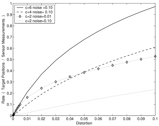
Figure 4: $C_{LB}(D)$ of arbitrary connections model for sensors of varying noise levels and range.

We compute the capacity bound $C_{LB}(D)$ in (1) for various distortions, noise levels, and sensor ranges. A sensor of range $c$ is connected to $c$ target positions. We assume that the sensing function $\Psi$ simply counts the number of target positions in the sensor range with a target present. The sensor noise model assumes that the probability of counting error decays exponentially with the error magnitude. In the figures, ‘Noise = $p$’ indicates that for a sensor, $P(Y\neq X)=p$, with ${\cal Y}={\cal X}$ assumed. In Figure 4, we demonstrate $C_{LB}(D)$ for various sensor noise levels and ranges. We compute this bound by systematically sampling the space of possible $\boldsymbol{\lambda}$. While $\boldsymbol{\lambda}$ is a four-dimensional vector, because of constraints we need to sample only two dimensions in order search over all valid $\boldsymbol{\lambda}$. In all cases, $C_{LB}(D)$ approaches $0$ as $D$ approaches $0$. This occurs because similar target vectors have similar codewords due to dependence in the codeword distribution. The relative magnitude of the bounds for sensors of various $c$ and noise levels describes tradeoffs among sensor types that can be captured by our result. Some tradeoffs are intuitive. For example, lower noise sensor of range $c$ have a higher sensing capacity than higher noise sensors of the same range. Other tradeoffs are more complex. For example the tradeoff between shorter and longer range sensors depends on the desired distortion. Sensors of range $4$ and noise $0.10$ result in a higher sensing capacity than sensors of range $2$ and noise $0.01$ for distortion above $0.047$. The opposite is true for distortions below $0.047$. Thus, the bound presented in (1) describes a complex tradeoffs between sensor noise, sensor range, and the desired detection accuracy.

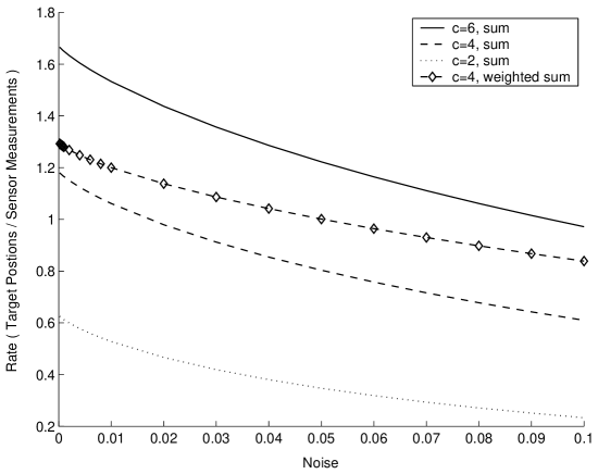
Figure 5: $C_{LB}(0.1)$ of arbitrary connections model for sensors of varying noise levels, range, and sensing function.

Figure 5 shows $C_{LB}(D)$ at $D=0.1$ as a function of sensor noise level for sensors of various range and sensing functions. This figure demonstrates that the strategy of simple sensor replication, which is a popular practical method for reducing error probability, can be inefficient. For example, for sensors of range $4$ and a sum sensing function, a rate of $0.61$ is achievable at noise level $0.1$. If each sensor with noise $0.1$ is replicated three times and majority decoding is used, the noise can be reduced to $3\times(0.1)^{2}\times 0.9+(0.1)^{3}=0.028$. For a noise level of $0.028$, $C_{LB}(0.1)$ equals $0.91$ for a sensor of range $4$ and a sum sensing function. However, due to sensor replication, the rate is reduced to $0.91/3=0.303$. This rate is significantly lower than the rate of $0.61$ for sensors of noise $0.1$ achievable by using our random sensor network construction. Thus, the bound indicates that cooperative sensor strategies can require significantly fewer sensor measurements than sensor replication. Figure 5 also shows $C_{LB}(D)$ at $D=0.1$ for sensors with $c=4$ and a weighted sum sensing function with weights $\{1,0.5,0.25,0.1\}$. This sensing function has a higher sensing capacity than sensors with the same range and an un-weighted sum sensing function across all noise levels. We conjecture that this occurs because a weighted sum can distinguish among more target configurations than an un-weighted sum. Interestingly, the gap between the two sensing functions increases with increasing noise.

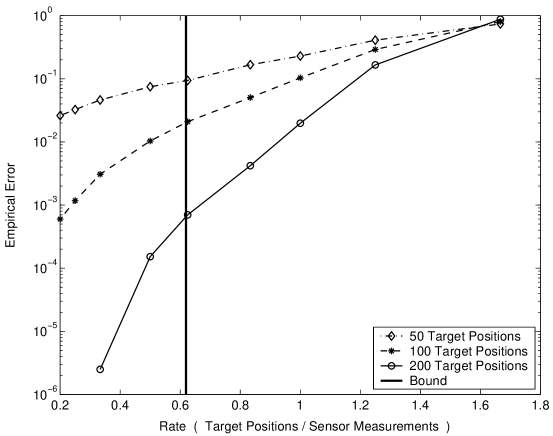
Figure 6: Average empirical error rate of belief propagation based detection for varying rates, and the corresponding sensing capacity bound.

Using the loopy belief propagation algorithm [35] we empirically examined sensor probability of error as a function of rate. We generated sensor networks of various rates by setting the number of targets, and varying the number of sensors. We chose the number of connections to be $c=4$, the distortion level to be $0.1$, and the noise level to be $0.1$ (i.e. $P(Y\neq X)=0.1$, with ${\cal Y}={\cal X}$). As in the previous section, we assume that the probability of error decays exponentially with error magnitude. We empirically evaluated the average error rate obtained in decoding target vectors in a randomly generated set of sensor networks. We plotted the average error rate for each rate value, and for various numbers of targets as shown in Figure 6. As the number of targets increase, the transition from high error to low error rate becomes increasingly sharp. However, all the error curves are well below the capacity value $C_{LB}(0.1)=0.62$. We conjecture that this occurs because belief propagation is suboptimal for graphs with cycles.

IV-E Extensions

Section IV-A introduced a sensor network model where each sensor is allowed to make arbitrary connections to the target vector. In several situations, more complex sensor network models may be necessary. This section describes extensions of the arbitrary connection model. Extensions that account for contiguity in sensor connections require a new model and are discussed in Section V. The first extension considers non-binary target vectors. Binary target vectors indicate the presence or absence of targets at the spatial positions. A target vector over a general finite alphabet may indicate, in addition to the presence of targets, the class of a target. Alternatively, the entries of non-binary vectors can indicate levels of intensity or concentration. Assuming a non-binary target vector, we can define types and joint types over an alphabet $\mathcal{V}$, and apply the same analysis as before to obtain the sensing capacity bound below.

$$C(D)\geq C_{LB}(D)=\min_{\begin{subarray}{c}\boldsymbol{\lambda}\\ \sum_{a\neq b}\lambda_{ab}\geq D\\ \sum_{b}\lambda_{ab}=\gamma_{a}\end{subarray}}\frac{D\left(P_{X_{i}Y}^{\boldsymbol{\gamma}}\|Q_{{X_{i}Y}}^{\boldsymbol{\lambda}}\right)}{H(\boldsymbol{\lambda})-H(\boldsymbol{\gamma})}$$ (15)

where ${\boldsymbol{\gamma}}=\left(\gamma_{a}=\frac{1}{|\mathcal{V}|},a\in\mathcal{V}\right)$, while $\boldsymbol{\lambda}=(\lambda_{ab},\ a,b\in\mathcal{V})$ is an arbitrary probability mass function.

The second extension allows the following a priori distribution over target vectors. Assume that each target position is generated i.i.d. with probability $P_{V}$ over the alphabet $\mathcal{V}$. This may model the fact that targets are sparsely present. The previous analysis can be extended to a Maximum-a-Posteriori (MAP) detector, instead of the ML detector considered earlier, resulting in the following sensing capacity bound.

$$C(D)\geq C_{LB}(D)=\min_{\begin{subarray}{c}\boldsymbol{\lambda}\\ \sum_{a\neq b}\lambda_{ab}\geq D\\ \sum_{b}\lambda_{ab}=\gamma_{ia}\end{subarray}}\frac{D\left(P_{X_{i}Y}^{\boldsymbol{\gamma}_{i}}\|Q_{{X_{i}Y}}^{\boldsymbol{\lambda}}\right)}{H(\boldsymbol{\lambda})-H(\boldsymbol{\gamma}_{j})-D(\boldsymbol{\gamma}_{j}\|P_{V})}$$ (16)

where ${\boldsymbol{\gamma}_{i}}=P_{V}$, $\boldsymbol{\lambda}=(\lambda_{ab},\ a,b\in\mathcal{V})$ is an arbitrary probability mass function and $\boldsymbol{\gamma}_{j}$ is the marginal of $\boldsymbol{\lambda}$ calculated as $\gamma_{jb}=\sum_{a}\lambda_{ab}$.

A third extension accounts for heterogenous sensors, where each class of sensor possibly has a different range $c$, noise model $P_{Y|X}$, and/or sensing function $\Psi$. Let the sensor of class $l$ be used with a given relative frequency $\alpha_{l}$. For such a model the sensing capacity bound is as follows.

$$C(D)\geq C_{LB}(D)=\min_{\begin{subarray}{c}\boldsymbol{\lambda}\\ \sum_{a\neq b}\lambda_{ab}\geq D\\ \sum_{b}\lambda_{ab}=\gamma_{ia}\end{subarray}}\frac{\sum_{l}\alpha_{l}D\left(P_{X_{i}Y}^{\boldsymbol{\gamma}_{i},l}\|Q_{{X_{i}Y}}^{\boldsymbol{\lambda},l}\right)}{H(\boldsymbol{\lambda})-H(\boldsymbol{\gamma}_{j})-D(\boldsymbol{\gamma}_{j}\|P_{V})}$$ (17)

where ${\boldsymbol{\gamma}_{i}}=P_{V}$, $\boldsymbol{\lambda}=(\lambda_{ab},\ a,b\in\mathcal{V})$ is an arbitrary probability mass function and $\boldsymbol{\gamma}_{j}$ is the marginal of $\boldsymbol{\lambda}$ calculated as $\gamma_{jb}=\sum_{a}\lambda_{ab}$.

V Sensing Capacity of Contiguous Connections Model

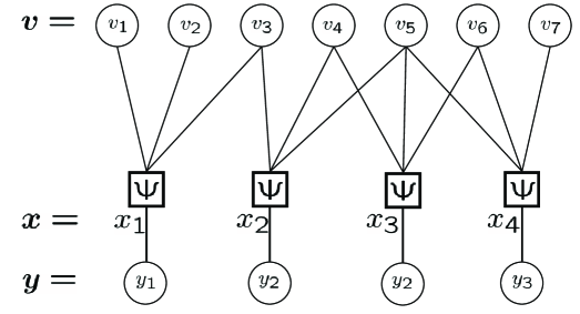
Figure 7: Sensor network model with $k=7,n=3,c=3$, contiguous connections, and a sensing function corresponding to the weighted sum of the observed targets.

In this section, we analyze the sensing capacity of a sensor network model that models contiguity in a sensor’s connections. Figure 7 shows an example of such a model. Sensor $\ell$ is connected to exactly $c$ contiguous positions out of the $k$ spatial positions. In contrast, the arbitrary connections model analyzed in the previous section did not account for localized sensor observations since each sensor could sense any $c$ (not necessarily contiguous) spatial positions.

V-A Higher Order Types

The statement of the result for contiguous models requires higher order types [11]. We introduce circular c-order types and circular c-order joint types. We define the circular $c$-order type of a binary sequence (i.e. a target vector) as a $2^{c}$ dimensional vector, $\boldsymbol{\gamma}$, where each entry in the vector corresponds to the frequency of occurrence of one of the possible subsequences of length $c$. A circular sequence is one in which the last element of the sequence precedes the first element of the sequence. The total number of subsequences of length $c$ that can occur in a circular sequence of length $k$ is $k$. For example, for a binary target vector and $c=2$, $\boldsymbol{\gamma}=(\gamma_{00},\gamma_{01},\gamma_{10},\gamma_{11})$. While it is possible to prove our bound using non-circular types as shown in [36], circular types lead to the same asymptotic result with the benefit of significantly simpler notation. The notational simplicity arises out of the fact that the lower order circular types are precise marginals of the higher order circular types. Although all the types in this section are circular, we will omit the word ‘circular’ when referring to types in the remainder of this section for brevity.

We denote the set of all $c$-order types over the alphabet $\mathcal{V}^{c}$ for target vectors of length $k$ as $\mathcal{P}_{k}(\mathcal{V}^{c})$. Since each sensor independently chooses a block of $c$ contiguous spatial positions, the distribution of its ideal output $X_{i}$ depends only on the $c$-order type $\boldsymbol{\gamma}$ of the target vector $\boldsymbol{v_{i}}$ which occurs. For a sensing function $\Psi$ and a target vector $\boldsymbol{v_{i}}$ of type $\boldsymbol{\gamma}$,

$$P_{X_{i}}(X_{i}=x)=\sum_{\begin{subarray}{c}\boldsymbol{a}\in\mathcal{V}^{c}\\ \Psi(\boldsymbol{a})=x\end{subarray}}\gamma_{\boldsymbol{a}}\doteq P^{\boldsymbol{\gamma}}(x)$$ (18)

Next, we note that the joint distribution $P_{\boldsymbol{X_{i}}\boldsymbol{X_{j}}}$ depends on the c-order joint type $\boldsymbol{\lambda}$ of the $i^{th}$ and $j^{th}$ target vectors $\boldsymbol{v_{i}},\boldsymbol{v_{j}}$. $\boldsymbol{\lambda}$ is the vector of $\lambda_{(\boldsymbol{a})(\boldsymbol{b})}$, the fraction of positions in $\boldsymbol{v_{i}},\boldsymbol{v_{j}}$ where $\boldsymbol{v_{i}}$ has a bit subsequence $\boldsymbol{a}$ while $\boldsymbol{v_{j}}$ has a bit subsequence $\boldsymbol{b}$. For example, when $c=2$ and $\mathcal{V}=\{0,1\}$, $\boldsymbol{\lambda}=(\lambda_{(00)(00)},\ldots,\lambda_{(11)(11)})$. We denote the set of all c-order joint types over the alphabet $\mathcal{V}^{c}$ for target vectors of length $k$ as $\mathcal{P}_{k}(\mathcal{V}^{c},\mathcal{V}^{c})$. Each $\boldsymbol{\lambda}\in\mathcal{P}_{k}(\mathcal{V}^{c},\mathcal{V}^{c})$ must satisfy the normalization constraint that the sum over all entries of $\lambda$ equals one. Since the joint type $\boldsymbol{\lambda}$ also defines the type $\boldsymbol{\gamma}$ of $\boldsymbol{v_{i}}$, for all $\{\boldsymbol{a}\}\in\mathcal{V}^{c}$ we must have $\gamma_{\boldsymbol{a}}=\sum_{\boldsymbol{b}\in\mathcal{V}^{c}}\lambda_{(\boldsymbol{a})(\boldsymbol{b})}$. Taking advantage of the fact that for circular types, lower order types are precise marginals of higher order types, we denote $\lambda_{(a)(b)}=\sum_{\boldsymbol{a}^{\prime}\in\mathcal{V}^{c-1}}\sum_{\boldsymbol{b}^{\prime}\in\mathcal{V}^{c-1}}\lambda_{(a\boldsymbol{a}^{\prime})(b\boldsymbol{b}^{\prime})}$. $\lambda_{(a)(b)}$ is the normalized count of locations where target vector $i$ has value $a$ while target vector $j$ has value $b$. Since each sensor depends only on the $c$ contiguous targets bits which it senses, $P_{\boldsymbol{X_{i}},\boldsymbol{X_{j}}}$ depends only on the joint type $\boldsymbol{\lambda}$. For target vectors $\boldsymbol{v_{i}}$,$\boldsymbol{v_{j}}$ of c-order joint type $\boldsymbol{\lambda}$,

$$P_{X_{i}X_{j}}(X_{i}=x_{i},X_{j}=x_{j})=\sum_{\begin{subarray}{c}\boldsymbol{a},\boldsymbol{b}\in\mathcal{V}^{c}\\ \Psi(\boldsymbol{a})=x_{i},\ \Psi(\boldsymbol{b})=x_{j}\end{subarray}}\lambda_{(\boldsymbol{a})(\boldsymbol{b})}\doteq P^{\boldsymbol{\lambda}}(x_{i},x_{j})$$ (19)

For example, for binary target vectors and $c=2$, vectors $00000000,01101000,01000111$ have $\boldsymbol{\gamma}=(1,0,0,0),(3/8,2/8,2/8,1/8),(2/8,2/8,2/8,2/8)$ respectively. Table IV contains the 2-order joint type of two target vectors. Consider a sensor network where each sensor is randomly connected to $c=2$ contiguous spatial positions. We assume that $\Psi$ outputs the number of targets which the sensor observes. Thus, each sensor has an ideal output alphabet $\mathcal{X}=\{0,1,2\}$. For target vectors of type $\boldsymbol{\gamma}$, $P(X_{i}=0)=\gamma_{00},P(X_{i}=1)=\gamma_{01}+\gamma_{10},P(X_{i}=2)=\gamma_{11}$ respectively. Given two target vectors $\boldsymbol{v_{i}},\boldsymbol{v_{j}}$ of joint type $\boldsymbol{\lambda}$, a sensor will output ‘0’ for both target vectors only if both of its connections see a ‘0’ bit in both target vectors. This happens with probability $\lambda_{(00)(00)}$. Table V lists the joint p.m.f. $P_{X_{i}X_{j}}(x_{i},x_{j})=P^{\boldsymbol{\lambda}}(x_{i},x_{j})$ for all output pairs $x_{i},x_{j}$ corresponding to joint type $\boldsymbol{\lambda}$. The table shows that $X_{i},X_{j}$ are not independent, in general.

To prove Theorem 1, we bounded the number of target vectors $\boldsymbol{v_{j}}$ that have a given joint type with a target vector $\boldsymbol{v_{i}}$ in equation (9). To prove a sensing capacity bound for the contiguous connections model we prove a bound on the number of target vectors $\boldsymbol{v_{j}}$ that have a joint c-order type $\boldsymbol{\lambda}$ with a target vector of $c$-order type $\boldsymbol{\gamma}$ in the lemma below. Before proceeding, we introduce the following notation. The set of length $k$ target vectors of $c$-order type $\boldsymbol{\gamma}$ is denoted $\mathcal{T}_{\boldsymbol{\gamma}}^{k}$. The set of pairs of length $k$ target vectors of joint type $\boldsymbol{\lambda}$ is denoted $\mathcal{T}_{\boldsymbol{\lambda}}^{k}$. The set of length $k$ target vectors that have joint c-order type $\boldsymbol{\lambda}$ with a given vector of type $\boldsymbol{\gamma}$, is denoted $\mathcal{T}_{\boldsymbol{\lambda}|\boldsymbol{\gamma}}^{k}$.

Lemma 1 (Bound on $|\mathcal{T}_{\boldsymbol{\lambda}|\boldsymbol{\gamma}}^{k}|$ )

The number of binary vectors of length $k$ with c-order joint type $\boldsymbol{\lambda}$ for a given vector of $c$-order type $\boldsymbol{\gamma}$, denoted $|\mathcal{T}_{\boldsymbol{\lambda}|\boldsymbol{\gamma}}^{k}|$, is bounded as follows

$$|\mathcal{T}_{\boldsymbol{\lambda}|\boldsymbol{\gamma}}^{k}|\leq C(k)2^{k(H(\boldsymbol{\tilde{\lambda}}|\boldsymbol{\lambda}^{\prime})-H(\boldsymbol{\tilde{\gamma}}|\boldsymbol{\gamma}^{\prime}))}$$ (20)

$C(k)=2^{2(c-1)}k^{2^{c-1}}(k+1)^{2^{2(c-1)}}$ and $\boldsymbol{\lambda}^{\prime}=\{\lambda_{(\boldsymbol{a})(\boldsymbol{b})},\forall\boldsymbol{a},\boldsymbol{b}\in\mathcal{V}^{c-1}\}$ is a probability mass function defined as $\lambda_{(\boldsymbol{a})(\boldsymbol{b})}^{\prime}=\sum_{a,b\in\mathcal{V}}\lambda_{(\boldsymbol{a}a)(\boldsymbol{b}b)}$. $\boldsymbol{\tilde{\lambda}}=\{\tilde{\lambda}_{(\boldsymbol{a}a)(\boldsymbol{b}b)},\forall\boldsymbol{a},\boldsymbol{b}\in\mathcal{V}^{c-1},\forall a,b\in\mathcal{V}\}$ is a conditional probability mass function defined as $\tilde{\lambda}_{(\boldsymbol{a}a)(\boldsymbol{b}b)}=\frac{\lambda_{(\boldsymbol{a}a)(\boldsymbol{b}b)}}{\lambda_{(\boldsymbol{a})(\boldsymbol{b})}}$. $\boldsymbol{\gamma}^{\prime}=\{\gamma_{\boldsymbol{a}}^{\prime},\forall\boldsymbol{a}\in\mathcal{V}^{c-1}\}$ is probability mass function defined as $\gamma_{\boldsymbol{a}}^{\prime}=\sum_{a\in\mathcal{V}}\gamma_{\boldsymbol{a}a}$. $\boldsymbol{\tilde{\gamma}}=\{\tilde{\gamma}_{\boldsymbol{a}a},\forall\boldsymbol{a}\in\mathcal{V}^{c-1},\forall a\in\mathcal{V}\}$ is a conditional probability mass function defined as $\tilde{\gamma}_{\boldsymbol{a}a}=\frac{\gamma_{\boldsymbol{a}a}}{\gamma_{\boldsymbol{a}}}$.

Proof:

To bound $|\mathcal{T}_{\boldsymbol{\lambda}|\boldsymbol{\gamma}}^{k}|$, we begin by bounding $|\mathcal{T}_{\boldsymbol{\gamma}}^{k}|$. The $c$-order type $\boldsymbol{\gamma}$ of a binary vector specifies a 2-order type (referred to as a Markov type) of a vector who entries are in an alphabet of cardinality $2^{c-1}$. Consider the vector $011010001$. Denoting a pair of bits using $\{0,1,2,3\}$, as we move from left to right over this vector, one bit at a time, the sequence obtained is $132120012$. The 3-order type $\boldsymbol{\gamma}$ specifies the 2-order type over this new vector. For example, the fraction of times $1$ transitions to $3$ is equal to $\gamma_{011}$ and the fraction of times $1$ transitions to $2$ is equal to $\gamma_{010}$. Any c-order type over a binary sequence can thus be mapped to a 2-order type over a sequence with symbols in an alphabet of cardinality $2^{c-1}$. [37] proves bounds on the number of sequences that correspond to a 2-order circular type over a sequence with an alphabet $\mathcal{V}$. Given our mapping from a c-order type to a 2-order type, we can apply this result to obtain the following bound,

$$|\mathcal{T}_{\boldsymbol{\gamma}}^{k}|\geq C_{1}(k)2^{k(H(\boldsymbol{\gamma})-H(\boldsymbol{\gamma}^{\prime}))}=C_{1}(k)2^{kH(\boldsymbol{\tilde{\gamma}}|\boldsymbol{\gamma}^{\prime})}$$ (21)

where $C_{1}(k)=k^{-2^{c-1}}(k+1)^{-2^{2(c-1)}}$. We now bound $|\mathcal{T}_{\boldsymbol{\lambda}}^{k}|$ using a similar argument. The c-order joint type $\boldsymbol{\lambda}$ of a pair of binary vectors specifies a 2-order type of a single vector whose entries are symbols from an alphabet of cardinality $2^{2(c-1)}$. We consider an example for a 3-order joint type, and for vectors $\boldsymbol{v}=011010001$ and $\boldsymbol{v}^{\prime}=101011011$. We can rewrite these vectors as a single vector whose entries at location $i$ are defined by the pair of entries $v_{i},v_{i}^{\prime}$ and the subsequent pair of entries $v_{i+1},v_{i+1}^{\prime}$. These four entries, combined as $v_{i}v_{i+1}v_{i}^{\prime}v_{i+1}^{\prime}$ are mapped to a symbol in an alphabet of cardinality $2^{4}$ by reading the entries as a binary number (i.e. $0000=0$, $0001=1$, $\ldots$). In this manner, $\boldsymbol{v}$ and $\boldsymbol{v}^{\prime}$ are mapped to a vector $(6,14,10,9,11,2,1,7,11)$. The 3-order joint type $\boldsymbol{\lambda}$ specifies the 2-order type over this new vector. For example, the fraction of times $1$ transitions to $7$ is equal to $\lambda_{(001)(011)}$ and the fraction of times $2$ transitions to $1$ is equal to $\lambda_{(000)(101)}$. Any c-order joint type over a binary sequence can thus be mapped to a 2-order type over a sequence with symbols in an alphabet of cardinality $2^{2(c-1)}$. We use the results of [37] again. Given our mapping from a c-order joint type to a 2-order type, we can apply this result to obtain the following bound,

$$|\mathcal{T}_{\boldsymbol{\lambda}}^{k}|\leq C_{2}2^{k(H(\boldsymbol{\lambda})-H(\boldsymbol{\lambda}^{\prime}))}=C_{2}2^{kH(\boldsymbol{\tilde{\lambda}}|\boldsymbol{\lambda}^{\prime})}$$ (22)

where $C_{2}=2^{2(c-1)}$. We observe that $|\mathcal{T}_{\boldsymbol{\lambda}|\boldsymbol{\gamma}}^{k}|$ depends only on the type $\boldsymbol{\gamma}$ of the vector on which we are conditioning, and not on the actual vector. Therefore, $|\mathcal{T}_{\boldsymbol{\lambda}|\boldsymbol{\gamma}}^{k}|=\frac{|\mathcal{T}_{\boldsymbol{\lambda}}^{k}|}{|\mathcal{T}_{\boldsymbol{\gamma}}^{k}|}$. Using equations (21) and (22), we obtain the following bound,

$$|\mathcal{T}_{\boldsymbol{\lambda}|\boldsymbol{\gamma}}^{k}|\leq C(k)2^{k(H(\boldsymbol{\tilde{\lambda}}|\boldsymbol{\lambda}^{\prime})-H(\boldsymbol{\tilde{\gamma}}|\boldsymbol{\gamma}^{\prime}))}$$ (23)

where $C(k)=C_{1}^{-1}(k)C_{2}$

∎

V-B Sensing Capacity Lower Bound

We define $P_{{X_{i}Y}}^{\boldsymbol{\gamma}}$ $Q_{{X_{i}Y}}^{\boldsymbol{\lambda}}$ as they were defined for the arbitrary connections model bounds, with the only difference arising to the use of $c$-order types instead of types.

Theorem 2 (Sensing Capacity Theorem for the Contiguous Connections Model)

The sensing capacity at distortion $D$ satisfies,

$$C(D)\geq C_{LB}(D)=\min_{\begin{subarray}{c}\boldsymbol{\lambda}\\ \lambda_{(0)(1)}+\lambda_{(1)(0)}\geq D\\ \end{subarray}}\frac{D\left(P_{X_{i}Y}^{\boldsymbol{\gamma}}\|Q_{{X_{i}Y}}^{\boldsymbol{\lambda}}\right)}{H(\boldsymbol{\tilde{\lambda}}|\boldsymbol{\lambda}^{\prime})-H(\boldsymbol{\tilde{\gamma}}|\boldsymbol{\gamma}^{\prime})}$$ (24)

where $\boldsymbol{\lambda}\in\mathcal{P}(\{0,1\}^{c},\{0,1\}^{c})$, $\boldsymbol{\gamma}_{\boldsymbol{a}}=\sum_{\boldsymbol{b}\in\{0,1\}^{c}}\lambda_{(\boldsymbol{a})(\boldsymbol{b})}$, and $H(\boldsymbol{\tilde{\gamma}}|\boldsymbol{\gamma}^{\prime})=1$.

If we specialize this result to the case of $c=1$, this theorem provides a bound that coincides with our bound for the arbitrary connections model. The proof of the sensing capacity lower bound is similar for the arbitrary and contiguous connections models. The main differences in the proofs arise due to the contiguity of sensor field of view, which necessitates the use of $c$-order types. Extensions demonstrated in Section IV-E for the arbitrary connections model can be easily applied to the contiguous connections model.

Proof Outline: The proof of Theorem 2 is essentially identical to the proof of Theorem 1, with types and joint types replaced by $c$-order types and joint types. The use of these higher order types requires counting arguments described in Lemma 1. For $c$-order types, we bound $\alpha$ in equation (7) as follows,

$$\alpha(\boldsymbol{\gamma},k)=|\mathcal{T}_{\boldsymbol{\gamma}}^{k}|\leq 2^{kH(\boldsymbol{\tilde{\gamma}}|\boldsymbol{\gamma}^{\prime})}$$ (25)

For c-order joint types, we bound $\beta(\boldsymbol{\lambda},k)=|\mathcal{T}_{\boldsymbol{\lambda}|\boldsymbol{\gamma}}^{k}|$ in equation (7) using Lemma 1. The set $S_{\boldsymbol{\gamma}}(D)$ is defined as,

$$S_{\boldsymbol{\gamma}}(D)=\Bigg{\{}\boldsymbol{\lambda}:\lambda_{0}+\lambda_{1}\geq D,\ \boldsymbol{\gamma}_{\boldsymbol{a}}=\sum_{\boldsymbol{b}\in\{0,1\}^{c}}\lambda_{(\boldsymbol{a})(\boldsymbol{b})}\Bigg{\}}$$ (26)

Given these new bounds and definitions, and the substitution of c-order types for types, the proof of Theorem 1 can be applied directly to prove Theorem 2.

V-C Numerical Results

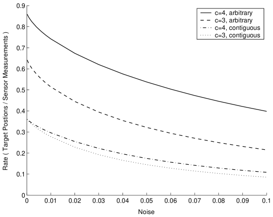
Figure 8: $C_{LB}(0.025)$ for localized and non-localized sensors.

In Figure 8, we compare $C_{LB}(D=0.025)$ for sensor networks with localized (i.e. contiguous connections model) and non-localized (i.e. arbitrary connections model) sensing. We assume that the sensing function $\Psi$ is a weighted additive function, with weights $\{1,0.5,0.25,0.1\}$ for $c=4$ and $\{1,0.5,0.25\}$ for $c=3$. The sensor noise model used throughout this section assumes that the probability of error decays exponentially with the error magnitude. In the figures, ‘Noise = $p$’ indicates that for a sensor, $P(Y\neq X)=p$, with ${\cal Y}={\cal X}$ assumed. Contiguous sensor field of view causes a significant reduction in sensing capacity. We conjecture that this effect is similar to the inferior performance of channel codes that have finite memory, such as convolutional codes, as opposed to LDPC codes. Further, it is interesting to note that the gap in sensing capacity between sensors of range $c=3$ and $c=4$ is larger for the arbitrary connections model than the contiguous connections model.

To compute the bound shown in Theorem 2, we solve a sequence of convex optimization problems. Rather than computing the bound directly, we find the largest $R$ for which the minimum of $f(\boldsymbol{\lambda})=D\left(P_{X_{i}Y}^{\boldsymbol{\gamma}}\|Q_{{X_{i}Y}}^{\boldsymbol{\lambda}}\right)-R(H(\boldsymbol{\tilde{\lambda}}|\boldsymbol{\lambda}^{\prime})-H(\boldsymbol{\tilde{\gamma}}|\boldsymbol{\gamma}^{\prime}))$ over all valid $\boldsymbol{\lambda}$ is greater than $0$. Minimizing $f(\boldsymbol{\lambda})$ is a convex optimization problem since $f(\boldsymbol{\lambda})$ is convex in $\boldsymbol{\lambda}$ and the set of valid $\boldsymbol{\lambda}$ is convex. Since $H(\boldsymbol{\tilde{\gamma}}|\boldsymbol{\gamma}^{\prime})=1$, the convexity of $f(\boldsymbol{\lambda})$ in $\boldsymbol{\lambda}$ can be proven using the log-sum inequality and the concavity of entropy.

V-D Extension to Two-dimensional Fields

The sensing capacity bounds obtained in this section can be extended from discrete target vectors to two dimensional ‘target fields.’ This extension requires the introduction of two dimensional types. Such types are histograms over the set of possible two dimensional patterns. We first analyzed the sensing capacity for a two-dimensional contiguous connections model in [38].

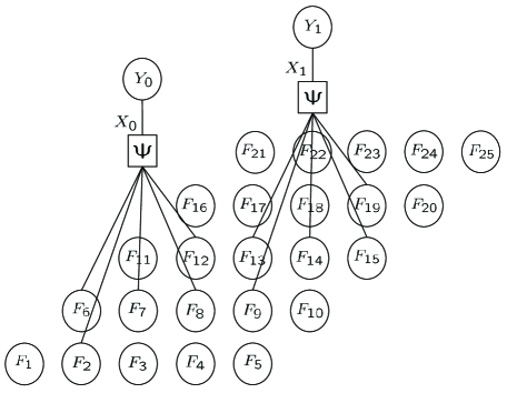
Figure 9: Sensor network model with $k=5,n=2,c=1$.

Figure 9 shows an example of our sensor network model. The state of the environment is modeled as a $k\times k$ grid with $k^{2}$ spatial positions. Each discrete position may contain no target or one target, and therefore the target configuration is represented by a $k^{2}$-bit target field $\boldsymbol{f}$. The possible target fields are denoted $\boldsymbol{f_{i}}$, $i\in\{1,\ldots,2^{k^{2}}\}$. Target fields occur with equal probability. The sensor network has $n$ identical sensors. Sensor $\ell$ located at grid block $F_{h}$ senses a set of contiguous target positions within a Euclidean distance $c$ of its grid location (though this approach can be extended to other sensor coverage models). Circular boundary conditions are assumed. Figure 9 depicts sensors with range $c=1$. Each sensor outputs a value $x\in{\cal X}$ that is an arbitrary function of the targets which it senses, $x=\Psi(\{f_{v}:v\in\mathcal{S}_{c,h}\})$, where $\mathcal{S}_{c,h}$ is the coverage of a sensor located at grid block $F_{h}$ with range $c$. Since the number of targets sensed by a sensor depends only on the sensor range, we write the number of targets in a sensor’s coverage as $|\mathcal{S}_{c}|$. We assume a simple model for randomly generating sensor networks, where each sensor chooses a region of Euclidean radius $c$ with equal probability among the set of possible regions of radius $c$. This would occur, for example, if sensors were randomly dropped on a field. All definitions from the one-dimensional contiguous model extend directly, with target vectors $\boldsymbol{v}$ replaced by fields $\boldsymbol{f}$. The rate is defined as $R=\frac{k^{2}}{n}$.

For a sensor located randomly in the target field, the probability of a sensor producing a value depends on the number of target patterns that correspond to that value in the sensor’s range, and thus, can be written as a function of the frequency of patterns in the field. The two-dimensional type $\boldsymbol{\gamma}_{i}$ is a vector that corresponds to the normalized counts over the set of possible target configurations in the sensor’s field of view in a field $\boldsymbol{f}_{i}$. For a sensor of range $c$, $\boldsymbol{\gamma}_{i}$ is a $2^{|\mathcal{S}_{c}|}$ dimensional vector, where each entry in the vector $\boldsymbol{\gamma}_{i}$ corresponds to the frequency of occurrence of one of the possible $|\mathcal{S}_{c}|$ bit patterns. The set of sensor types $\boldsymbol{\gamma}$ of a $k\times k$ field is denoted $\mathcal{P}_{k}^{2}(\{0,1\}^{|\mathcal{S}_{c}|})$. $\gamma_{(0)}$ and $\gamma_{(1)}$ are the number of zeros and ones respectively in a vector of type $\boldsymbol{\gamma}$. These quantities can be directly computed from $\boldsymbol{\gamma}$.

Next, we note that for sensor of range $c$ the conditional probability $P_{\boldsymbol{X_{i}}\boldsymbol{X_{j}}}$ depends on the two-dimensional joint type $\boldsymbol{\lambda}$ of the $i^{th}$ and $j^{th}$ target fields $\boldsymbol{f_{i}},\boldsymbol{f_{j}}$. For $\boldsymbol{a},\boldsymbol{b}\in\{0,1\}^{|\mathcal{S}_{c}|}$, $\boldsymbol{\lambda}$ is the matrix of $\lambda_{(\boldsymbol{a})(\boldsymbol{b})}$, the fraction of positions in $\boldsymbol{f_{i}},\boldsymbol{f_{j}}$ where $\boldsymbol{f_{i}}$ has a target pattern $\boldsymbol{a}$ while $\boldsymbol{f_{j}}$ has a target pattern $\boldsymbol{b}$. We denote the set of all joint sensor types for sensors of range $c$ observing a target field of area $k^{2}$, as $\mathcal{P}_{k}^{2}(\{0,1\}^{|\mathcal{S}_{c}|},\{0,1\}^{|\mathcal{S}_{c}|})$. Since the output of each sensor depends only on the contiguous region of targets which it senses, $P_{\boldsymbol{X_{i}}\boldsymbol{X_{j}}}$ depends only on $\boldsymbol{\lambda}$ (discussed in Section IV-B). $\lambda_{(1)(0)}$ is the number of grid locations where field $i$ has a target and field $j$ does not, and can be computed directly from $\boldsymbol{\lambda}$. $\lambda_{(0)(1)}$ is similarly defined and computed.

Using the definitions of two dimensional types in the definitions of $P_{X_{i}Y}^{\boldsymbol{\gamma}_{i}}$ and $Q_{{X_{i}Y}}^{\boldsymbol{\lambda}}$ from the one-dimensional contiguous connections model, we can prove the following bound for sensing a two-dimensional field. The sensing capacity at distortion $D$ satisfies,

$$C(D)\geq C_{LB}(D)=\min_{\begin{subarray}{c}\boldsymbol{\lambda}\\ \lambda_{(0)(1)}+\lambda_{(1)(0)}\geq D\end{subarray}}\frac{D\left(P_{X_{i}Y}^{\boldsymbol{\gamma}_{i}}\|Q_{{X_{i}Y}}^{\boldsymbol{\lambda}}\right)}{H((\gamma_{j(0)},\gamma_{j(1)}))}$$ (27)

where $\boldsymbol{\gamma}_{i},\boldsymbol{\gamma}_{j}\in\mathcal{P}^{2}(\{0,1\}^{|\mathcal{S}_{c}|})$, $\gamma_{i(0)}=0.5$ and $\gamma_{i(1)}=0.5$, and $\boldsymbol{\lambda}\in\mathcal{P}^{2}(\{0,1\}^{|\mathcal{S}_{c}|},\{0,1\}^{|\mathcal{S}_{c}|})$.

Proof Outline: The proof is essentially identical to the proof of Theorem 1, with types and joint types replaced by two-dimensional types and joint types. For two-dimensional types, we bound $\alpha$ as follows,

$$\alpha(\boldsymbol{\gamma}_{i},k)\leq 2^{k^{2}H((\gamma_{i(0)},\gamma_{i(1)}))}$$ (28)

For two-dimensional joint types, we bound $\beta$ as,

$$\beta(\boldsymbol{\lambda},k)\leq 2^{k^{2}H((\gamma_{j(0)},\gamma_{j(1)}))}$$ (29)

The bounds on $\alpha$ and $\beta$ are loose, and the authors are not aware of tighter combinatorial bounds for two-dimensional types. The set $S_{\boldsymbol{\gamma}}(D)$ is defined as in equation (26). Given these new bounds and definitions, and the substitution of 2D types for types, the proof of Theorem 1 can be applied directly to prove this result.

VI Conclusions and Discussion

The results presented in this paper provide limits on the accuracy of sensor networks for large-scale detection applications. These results are obtained by drawing on an analogy between channel coding and sensor networks. We define the sensing capacity and lower bound it for several sensor network models. For all rates below the sensing capacity, detection to within a desired accuracy with arbitrarily small error is achievable. This threshold behavior contrasts with classical detection problems, where probability of error goes to zero as the number of sensor measurements go to infinity while the number of hypotheses remains fixed [39]. The sensing capacity captures complex sensor tradeoffs. For example, our bounds show that the efficiency of using long range, noisy sensors or shorter range, less noisy sensors depends on the desired detection accuracy. Further, our results show that the mutual information is not the correct notion of information for large-scale detection problems. This has implications for the problem of sensor selection due to the popularity of ‘information gain’ as a sensor selection metric.

An important contribution of this paper is its demonstration of a close connection between sensor networks and communication channels. It is thought-provoking to consider that one could apply insights from the large body of work available for communication channels to the sensor network setting. For example, channel coding theory contains a large number of results that are used to build practical communication systems. Can we fruitfully apply ideas from coding theory to sensor networks? To demonstrate the potential benefit of a channel coding perspective, in [40, 41] we proposed extending ideas from convolutional coding to sensor networks. We demonstrated that a version of sequential decoding (a low complexity decoding heuristic for convolutional codes) can be applied to detection in sensor networks, as an alternative to the belief propagation algorithm. Our empirical results indicate that above a certain number of sensor measurements, the sequential decoding algorithm achieves accurate decoding with bounded computations per bit (target position). This empirical result suggests the existence of a ‘computational cut-off rate’, similar to one that exists for channel codes.

Our work on the theory of sensing points to a large set of open problems on large-scale detection. Obvious directions include strengthening the theory by considering alternative settings of the problem, tightening the sensing capacity bounds, and proving a converse to sensing capacity. For example, we presented extensions to the work presented in this paper by considering the impact of spatial [38] and temporal [42] dependence on the sensing capacity. Another direction for future work is to explore the connection between sensor networks and communication channels, including the exploitation of existing channel codes to design sensor networks.

$\boldsymbol{v_{j}}$	$\boldsymbol{\gamma}$ of $\boldsymbol{v_{j}}$	$\boldsymbol{\lambda}$ of $\boldsymbol{v_{j}}$ with $\boldsymbol{v_{i}}=0010110$
0010110	$\big{(}\frac{4}{7},\frac{3}{7}\big{)}$	$\big{(}\frac{4}{7},0,0,\frac{3}{7}\big{)}$
0000110	$\big{(}\frac{5}{7},\frac{2}{7}\big{)}$	$\big{(}\frac{4}{7},0,\frac{1}{7},\frac{2}{7}\big{)}$
1000011	$\big{(}\frac{4}{7},\frac{3}{7}\big{)}$	$\big{(}\frac{2}{7},\frac{2}{7},\frac{2}{7},\frac{1}{7}\big{)}$
0000000	$\big{(}1,0\big{)}$	$\big{(}\frac{5}{7},0,\frac{3}{7},0\big{)}$

TABLE I: Joint types $\boldsymbol{\lambda}$ for four pairs of target vectors.

$X_{i}$	$X_{i}=0$	$X_{i}=1$	$X_{i}=2$
$P_{X_{i}}$	$(\gamma_{0})^{2}$	$2\gamma_{0}\gamma_{1}$	$(\gamma_{1})^{2}$

TABLE II: Distribution of $X_{i}$ in terms of the type $\boldsymbol{\gamma}$ of $\boldsymbol{v_{i}}$ when $c=2$.

$P_{X_{i}X_{j}}$	$X_{j}=0$	$X_{j}=1$	$X_{j}=2$
$X_{i}=0$	$(\lambda_{00})^{2}$	$2\lambda_{00}\lambda_{01}$	$(\lambda_{01})^{2}$
$X_{i}=1$	$2\lambda_{00}\lambda_{10}$	$2\left(\lambda_{10}\lambda_{01}+\lambda_{00}\lambda_{11}\right)$	$2\lambda_{01}\lambda_{11}$
$X_{i}=2$	$(\lambda_{10})^{2}$	$2\lambda_{10}\lambda_{11}$	$(\lambda_{11})^{2}$

TABLE III: Joint distribution of $X_{j}$ and $X_{i}$ in terms of the joint type $\boldsymbol{\lambda}$ of $\boldsymbol{v_{i}},\boldsymbol{v_{j}}$ when $c=2$.

$\lambda_{(ab)(cd)}$	$cd=00$	$cd=01$	$cd=10$	$cd=11$
$ab=00$	0	0	1/8	2/8
$ab=01$	1/8	1/8	0	0
$ab=10$	1/8	1/8	0	0
$ab=11$	0	0	1/8	0

TABLE IV: $\boldsymbol{\lambda}$ with $c=2$ for $\boldsymbol{v_{i}}=01101000$ and $\boldsymbol{v_{j}}=01000111$.

$P_{X_{i}X_{j}}$	$X_{j}=0$	$X_{j}=1$	$X_{j}=2$
$X_{i}=0$	$\lambda_{(00)(00)}$	$\lambda_{(00)(01)}+\lambda_{(00)(10)}$	$\lambda_{(00)(11)}$
$X_{i}=1$	$\lambda_{(10)(00)}+\lambda_{(01)(00)}$	$\lambda_{(01)(01)}+\lambda_{(01)(10)}+\lambda_{(10)(01)}+\lambda_{(10)(10)}$	$\lambda_{(10)(11)}+\lambda_{(01)(11)}$
$X_{i}=2$	$\lambda_{(11)(00)}$	$\lambda_{(11)(01)}+\lambda_{(11)(10)}$	$\lambda_{(11)(11)}$

TABLE V: Joint distribution of $X_{j}$ and $X_{i}$ in terms of the joint type $\boldsymbol{\lambda}$ of $\boldsymbol{v_{j}}$ and $\boldsymbol{v_{i}}$, with $c=2$.

References

- [1] S. Thrun, “Robotic mapping: A survey,” in Exploring Artificial Intelligence in the New Millenium, G. Lakemeyer and B. Nebel, Eds. Morgan Kaufmann, 2002.
- [2] A. Elfes, “Occupancy grids: a probabilistic framework for mobile robot perception and navigation,” Ph.D. dissertation, Electrical and Computer Eng. Dept., Carnegie Mellon University, 1989.
- [3] R. Collins, A. Lipton, T. Kanade, H. Fujiyoshi, D. Duggins, Y. Tsin, D. Tolliver, N. Enomoto, and O. Hasegawa, “A system for video surveillance and monitoring,” Robotics Institute, Carnegie Mellon University, Pittsburgh, PA, Tech. Rep. CMU-RI-TR-00-12, May 2000.
- [4] A. Hoover and B. Olsen, “A real-time occupancy map from multiple video streams,” in Proc. Int. Conf. on Robotics and Automation, 1999.
- [5] M. Burl, B. Sisk, T. Vaid, and N. Lewis, “Classification performance of carbon black-polymer composite vapor detector arrays as a function of array size and detector composition,” Sensors and Actuators B, vol. 87, pp. 130–149, 2002.
- [6] D. Li, K. Wong, Y. Hu, and A. Sayeed, “Detection, classification and tracking of targets in distributed sensor networks,” IEEE Signal Processing Magazine, pp. 17–29, March 2002.
- [7] Y. Tian and H. Qi, “Target detection and classification using seismic signal processing in unattended ground sensor systems,” in International Conference on Acoustics Speech and Signal Processing (ICASSP), vol. 4, May 2002.
- [8] C. Shannon, “A mathematical theory of communication,” Bell System Technical Journal, vol. 27, pp. 379–423 and 623–656, July and October 1948.
- [9] Y. Rachlin, R. Negi, and P. Khosla, “Sensing capacity for target detection,” in Proc. IEEE Inform. Theory Wksp., Oct. 24-29 2004.
- [10] J. Manyika and H. Durrant-Whyte, Data Fusion and Sensor Management: A Decentralized Information-Theoretic Approach. Prentice Hall, 1994.
- [11] I. Csiszar, “The method of types,” IEEE Trans. Inform. Theory, vol. 44, no. 6, 1998.
- [12] E. J. Duarte-Melo and M. Liu, “Data-gathering wireless sensor networks: organization and capacity,” Computer Networks: Special Issue on Wireless Sensor Networks, vol. 43, 2003.
- [13] P. Gupta and P. R. Kumar, “The capacity of wireless networks,” IEEE Trans. Inform. Theory, vol. 46, no. 2, 2000.
- [14] G. Barrenechea, B. Beferull-Lozano, and M. Vetterli, “Lattice sensor networks: Capacity limits, optimal routing and robustness to failures,” in Third Int. Symp. Info. Proc. in Sensor Networks, Apr. 2004.
- [15] U. Mitra and A. Sabharwal, “Complexity constrained sensor networks: Achievable rates for two relay networks and generalizations,” in Third Int. Symp. Info. Proc. in Sensor Networks, Apr. 2004.
- [16] Z. Hu and B. Li, “Fundamental performance limits of wireless sensor networks,” in Ad Hoc and Sensor Networks, Y. Xiao and Y. Pan, Eds. Nova Science Publishers, 2004.
- [17] D. Slepian and J. Wolf, “Noiseless coding of correlated information sources,” IEEE Trans. Inform. Theory, vol. 19, pp. 471–480, 1973.
- [18] A. Wyner and J. Ziv, “The rate-distortion function for source coding with side information at the receiver,” IEEE Trans. Inform. Theory, vol. 22, pp. 1–10, 1976.
- [19] S. Pradhan, J. Kusuma, and K. Ramachandran, “Distributed compression in a dense microsensor network,” IEEE Signal Processing Magazine, vol. 19, pp. 51–60, March 2002.
- [20] Z. Xiong, A. Liveris, and S. Cheng, “Distributed source coding for sensor networks,” IEEE Signal Processing Magazine, vol. 21, pp. 80–94, 2004.
- [21] P. Varshney, Distributed Detection and Data Fusion. Springer-Verlag, 1997.
- [22] J. Chamberland and V. Veeravalli, “Decentralized detection in sensor networks,” IEEE Transactions on Signal Processing, vol. 51, no. 2, pp. 407–416, 2003.
- [23] ——, “Asymptotic results for decentralized detection in power constrained wireless sensor networks,” IEEE JSAC Special Issue on Wireless Sensor Networks, vol. 22, no. 6, pp. 1007–1015, 2004.
- [24] A. D’Costa, V. Ramachandran, and A. Sayeed, “Distributed classification of gaussian space-time sources in wireless sensor networks,” IEEE J. Selected Areas in Communications (special issue on Fundamental Performance Limits of Wireless Sensor Networks), pp. 1026–1036, Aug. 2004.
- [25] J. Kotecha, V. Ramachandran, and A. Sayeed, “Distributed multi-target classification in wireless sensor networks,” IEEE JSAC Special Issue on Self-Organizing Distributed Collaborative Sensor Networks, 2005.
- [26] K. Chakrabarty, S. S. Iyengar, H. Qi, and E. Cho, “Coding theory framework for target location in distributed sensor networks,” in Proc. Int. Conf. on Inform. Technology: Coding and Computing, April 2001.
- [27] A. Scaglione and S. D. Servetto, “On the interdependence of routing and data compression in multi-hop sensor networks,” in Proc. 8th ACM Int. Conference on Mobile Computing and Networking, Sept. 2002.
- [28] R. Nowak, U. Mitra, and R. Willett, “Estimating inhomogeneous fields using wireless sensor networks,” IEEE Journal on Selected Areas in Communications, vol. 22, no. 6, pp. 999–1006, August 2004.
- [29] D. Marco, E. Duarte-Melo, M. Liu, and D. Neuhoff, “On the many-to-one transport capacity of dense wireless sensor networks and the compressibility of its data,” in Information Processing in Sensor Networks, 2003, pp. 1–16.
- [30] P. Ishwar, A. Kumar, and K. Ramachandran, “Distributed sampling for dense sensor networks: A bit-conservation principle,” in Information Processing in Sensor Networks, 2003.
- [31] W. Bajwa, A. Sayeed, and R. Nowak, “Matched source-channel communication for field estimation in wireless sensor networks,” in Proc. Fourth Int. Symp. on Information Processing in Sensor Networks, April 25-27 2005.
- [32] A. Kumar, P. Ishwar, and K. Ramchandran, “On distributed sampling of smooth non-bandlimited fields,” in Int. Symp. on Information Processing in Sensor Networks, April 2004.
- [33] M. Gastpar and M. Vetterli, “Power, spatio-temporal bandwidth, and distortion in large sensor networks,” IEEE Journal on Selected Areas in Communications, vol. 23, no. 4, pp. 745–754, April 2005.
- [34] R. Gallager, Information Theory and Reliable Communications. Wiley, 1968.
- [35] J. Pearl, Probabilistic Reasoning in Intelligent Systems: Networks of Plausible Inference. Morgan Kaufmann, 1988.
- [36] Y. Rachlin, R. Negi, and P. Khosla, “Sensing capacity for discrete sensor network applications,” in Proc. Fourth Int. Symp. on Information Processing in Sensor Networks, April 25-27 2005.
- [37] L. Davisson, G. Longo, and A. Sgarro, “The error exponent for the noiseless encoding of finite ergodic markov sources,” IEEE Trans. Inform. Theory, vol. 27, pp. 431–438, 1981.
- [38] Y. Rachlin, R. Negi, and P. Khosla, “Sensing capacity for markov random fields,” in Proc. Int. Symp. on Information Theory, 2005.
- [39] T. M. Cover and J. A. Thomas, Elements of Information Theory. Wiley-Interscience, 1991.
- [40] Y. Rachlin, R. Negi, and P. Khosla, “On the interdependence of sensing and estimation complexity in sensor networks,” in Proc. Fifth Int. Conf. on Information Processing in Sensor Networks, April 19-21 2006.
- [41] Y. Rachlin, B. Narayanaswamy, R. Negi, J. Dolan, and P. Khosla, “Increasing sensor measurements to reduce detection complexity in large-scale detection applications,” in Proc. Military Communications Conference, 2006.
- [42] Y. Rachlin, R. Negi, and P. Khosla, “Temporal sensing capacity,” in Proc. Allerton Conference on Communication, Control, and Computing, 2006.