Physical Conditions in the Ionized Gas of 30 Doradus

Abstract

We present a mid-infrared spectroscopic data cube of the central part of 30 Doradus, observed with Spitzer’s IRS and MIPS/SED mode. Aromatic dust emission features and emission lines from molecular and atomic hydrogen are detected but not particularly strong. The dominant spectral features are emission lines from moderately ionized species of argon, neon, and sulphur, which are used to determine the physical conditions in the ionized gas. The ionized gas excitation shows strong variations on parsec scales, some of which can plausibly be associated with individual hot stars. We fit the ionic line strengths with photoionization and shock models, and find that photoionization dominates in the region. The ionization parameter $U$ traces the rim of the central bubble, as well as highlighting isolated sources of ionization, and at least one quiescent clump. The hardness of the ionizing radiation field $T_{rad}$ reveals several “hot spots” that are either the result of individual very hot stars or trace the propagation of the diffuse ionizing field through the surrounding neutral cloud. Consistent with other measurements of giant H II regions, log($U$) ranges between -3 and -0.75, and $T_{rad}$ between 30000 and 85000K.

1 Introduction

The 30 Doradus region of the Large Magellanic Cloud (LMC) is an ideal laboratory in which to study the effect of massive star formation and its feedback on the circumcluster interstellar medium (ISM). Star formation processes in the Magellanic Clouds are potentially a template for the early universe, where small irregular galaxies were commonplace and the overall metallicity lower. In particular, the star formation rate measured relative to molecular mass may be high in the LMC compared to our Galaxy, but that measurement is complicated by interpretation of CO data in molecular clouds that are known to be more porous and deeply penetrated by ultraviolet radiation, and an uncertain CO-H₂ conversion factor (e.g. Poglitsch et al., 1995; Bernard et al, 2008).

30 Doradus itself, the brightest star formation region in the LMC, contains several $10^{5}$M_⊙ of molecular hydrogen traced by ¹²CO(1-0) (Johansson et al., 1998), much of which is in two elongated clouds that form an arc or ridge in the center of the nebula (see Figure 1 for a multiwavelength view and Figure 2 for the distribution of CO). That molecular material is probably only the remnant of the cloud that formed the central cluster and thousands of OB stars. Observations of higher energy CO transitions suggest that this remnant ridge of molecular gas is quite warm and dense (Kim, 2007), and near-infrared observations have revealed that it is actively forming new stars (Hyland et al., 1992; Rubio et al., 1998; Maercker & Burton, 2005)

The dominant star-forming cluster of the 30 Doradus H II region is NGC 2070, whose dense center, R136, is usually considered the nearest super star cluster (SSC). R136 contains 39 O3 stars, a total stellar mass of $\simeq$5${}\times 10^{4}$M_⊙ within 2.5 pc, and stellar densities exceeding 5${}\times 10^{4}$M_⊙pc^-3 (Hunter, 1999; Walborn, 1991). Extragalactic SSCs are the hosts of one of the most extreme modes of star formation in the universe, may develop into globular clusters, and play a key role in galaxy formation (Johnson, 2004). At a distance of 50$\pm$2.5 kpc (see discussion of the LMC distance and uncertainty in Schaefer, 2008), 30 Doradus is close enough to study at the parsec-scale resolution that is required to understand the formation and feedback effects of individual stars, and a prime target for detailed study of the same mechanisms which operate in more distant and massive SSCs.

Observations at mid-infrared (MIR) wavelengths offer several advantages for studying star formation and its interaction with circumcluster dust and gas. MIR (here roughly defined as 5-50$\mu$m) continuum emission is generally dominated by radiation from very small dust grains (VSGs); the broad shape of the continuum is sensitive to the VSG size and temperature distribution, and hence indirectly to the radiation intensity in photon-dominated regions, and to the destruction of smaller grains as would be expected above 2000K and in H II regions. Broad ($\sim$1$\mu$m) dust emission features are also present between 3 and 19$\mu$m. These previously named “unidentified infrared bands” result from distortion (bending, stretching) modes of aromatic molecules containing tens to hundreds of carbon atoms. (Most features have been attributed to polycyclic aromatic hydrocarbons, PAHs, but unique astrophysical identification is a work in progress). Analysis of relative strengths of PAH features reveals their size and ionization state which is expected to change in intense radiation fields. Extinction by dust in the infrared is low compared to other wavelength regimes. Observations in the MIR can pierce cold molecular clouds and reveal the star-forming regions that they shroud. There are two major bands of absorption by silicate dust at 9.7 and 18$\mu$m, whose shape and strength provide further diagnostics of the dust in the region. Mid-infrared (MIR) spectroscopy of the entire 30 Doradus region with ISO-SWS (Sturm et al., 2000) revealed a continuum-dominated spectrum with very weak silicate absorption and also only modestly strong aromatic emission features. The 4 spectra taken in 30 Doradus with ISOPHOT (Vermeij et al., 2002) similarly show low ratios of PAH strength to IR continuum.

The most recent and sensitive MIR continuum observations of the Magellanic Clouds were obtained as part of the Spitzer (Werner et al., 2004) Legacy program “Surveying the Agents of a Galaxy’s Evolution” (SAGE), using IRAC (3–8$\mu$m; Fazio et al., 2004) and MIPS (24-160$\mu$m; Rieke et al., 2004). The goals of SAGE are to conduct a detailed study of the dust processes in the ISM, to complete a census of newly formed stars in order to find the star formation rate in the LMC, and to study evolved stars with high mass loss rates in order to determine the rate of mass injection into the ISM (Meixner et al., 2006). Figure 1 places the MIR emission from 30 Doradus in its multiwavelength context. 8$\mu$m emission traces the same arc-shaped ridge seen in the optical, delineating the edge of a bubble probably blown by R136 and filled with hot X-ray emitting plasma. The remaining molecular material in the region is also located in that ridge.

This paper presents a new spatially filled spectral cube of 30 Doradus with the low-resolution modules of Spitzer/IRS (Houck et al., 2004) and with the SED mode of Spitzer/MIPS (Rieke et al., 2004; Lu et al., 2008). The sensitivity of this dataset greatly exceeds the previous ISOCAM-CVF data (Madden et al., 2006), which only provided maps of the few strongest ionic lines, but tentatively showed a gradient of decreasing excitation in the [Ne III]/[Ne II] ratio as a function of distance from R136, and signs of PAH destruction in the central regions of the nebula.

The data are described in sections §2. In particular, §2.1 and Appendix A discusses reduction and artifacts, §2.3 the line and feature fitting procedure, and Appendix B quality assurance tests including a comparison with high-resolution IRS data from Lebouteiller et al. (2007). In §3.1 we describe the general results – the spatial distribution of emission lines and their ratios. §4 describes the derived distribution of matter – electron density and dust, and §5 the distribution of radiation evident in the excitation of the gas. We compare the data with photoionization and shock models, and summarize and discuss implications in §6.

2 Observations

The Spitzer’s Infrared Spectrograph has $\gtrsim$100 times greater spectroscopic sensitivity than the previous premier infrared observatory, ISO-SWS, and $\gtrsim$10 times higher spatial resolution than the SWS aperture size. We used the four low resolution modules of the IRS. The spectral resolution ranges from 60 to 120 (Spitzer Observer’s Manual 7.1, 2006), with reliable wavelength coverage as noted in section A.0.3. The four modules are the short wavelength / low resolution second order (SL2), short wavelength / low resolution first order (SL1), long wavelength / low resolution second order (LL2), and long wavelength / low resolution first order (LL1). Our data is divided into eighteen Astronomical Observing Requests (AORs), each containing many BCD (basic calibrated data) frames, which are pipeline-processed images of the IRS chip.

We observed 30 Doradus over five days in September of 2006, using Spitzer’s spectral mapping mode in order to obtain detailed spatial information. The total amount of time on target was 74 hours. We used 3440 slit pointings, covering 40.5 square arcminutes in the short-wavelength modules and 69.1 square arcminutes in the long-wavelength modules (see Figure 3). Each slit overlaps half of the preceding one, and each row of slits overlaps half of the preceding row, so every point on the map was observed at four separate slit pointings. There were three repetitions per pointing for the SL observations, at 14 seconds each (for a total time of 168 s for each point on the SL maps), and four repetitions per pointing for the LL observations, at 6 seconds each (for a total time of 96 s for each point on the LL maps). The result is four large and dense spectral cubes, one for each module.

We also made separate observations of a nearby region of comparatively blank sky, bracketing our target observations in time, to comprise background observations and to better characterize rogue pixel response. The total time on background was 44 minutes.

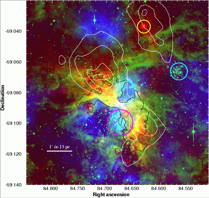
Figure 1: The 30 Doradus nebula. Red: IRAC 8$\mu$m image (SAGE). Green: ESO B-band image. Blue: broad-band soft X-ray image, $0.5-2$ keV (private correspondence and Townsley et al., 2006). All images are on a linear scale. White contours: ¹²CO(1-0) emission (Johansson et al., 1998). Black contour: a single level of 3cm radio emission, to guide the eye (see Figure 2). Magenta mark: the star cluster R136, core of NGC 2070, at 5^h38^m42^s -69^∘06′00″. Cyan mark: the star cluster Hodge 301, at 5^h38^m16^s -69^∘04′00″. Yellow mark: an IR point source in the molecular cloud [JGB98] Dor-06 (Johansson et al., 1998), at 5^h38^m31.63^s -69^∘02′14.6″. This source is also marked in white in Figure 4 and discussed in §2.2.

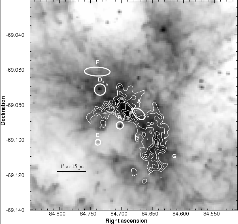
Figure 2: IRAC 8$\mu$m image (log scale). White contours: high-resolution 3cm continuum from Lazendic et al. (2003). Contour levels: 6, 9, 12, 15, 18, and 21 ${}\times 10^{-3}$ Jy/bm. Sources of interest marked here are listed in Table 2, described in §3.3, and their spectra shown in Figure 17.

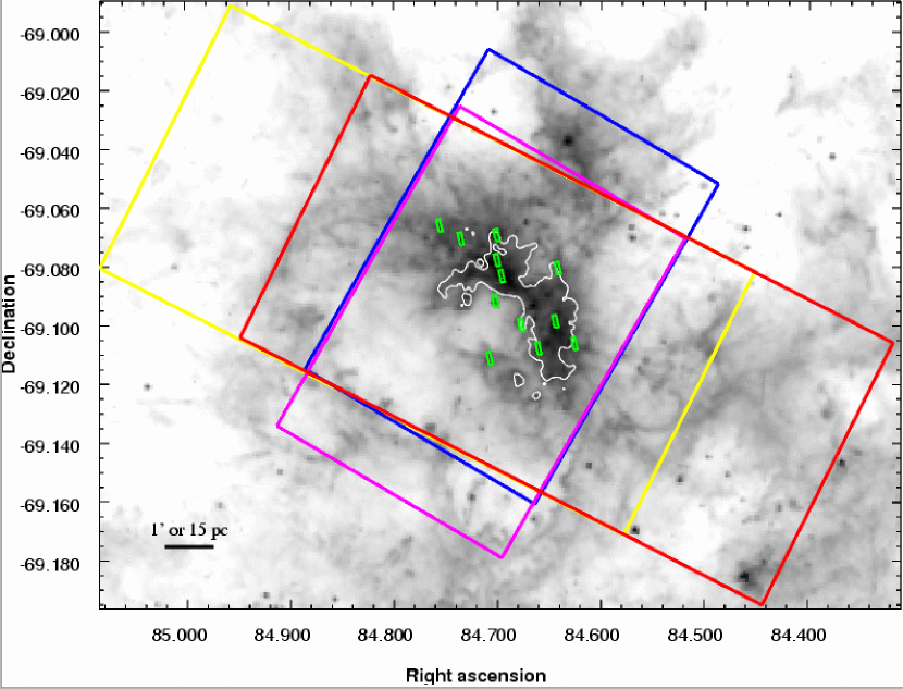
Figure 3: IRAC 8$\mu$m image with the scope of coverage in each of the IRS modules shown. Red: LL1. Yellow: LL2. Blue: SL1. Magenta: SL2. Green: high resolution GTO apertures (see Appendix B).

2.1 Reduction of IRS data cube

We used the basic calibrated data (BCD) from the Spitzer Science Center pipeline version S14.4.0. The main tool for the assembly and reduction of our data cube was CUBISM (Smith, 2007b), which is designed for spatially dense IRS maps. The functions of CUBISM include tools to reduce the data (subtracting background, applying a slit loss correction function, trimming the slit in the spatial direction, masking pixels that are flagged by the pipeline, and applying algorithms to identify rogue pixels) and to extract spectra and maps from the data cube.

Appendix A describes in detail our procedure for calibrating and adjusting the flux levels such that the different spectrograph modules could be combined into smooth spectra. In brief, we used contemporaneous off-source background observations to subtract the thermal background. We used measurements of the slit-loss correction function provided by the Spitzer Science Center to undo that part of their point-source-based calibration (since our observations are more similar to a uniform diffuse source than a point source). Finally, we adjusted spectra from different modules to match each other.

Appendix B describes our comparisons of high and low-resolution spectra in 30 Doradus to test the fidelity of our fitting process. We find that the strengths of even somewhat blended lines are recovered well in the low-resolution spectra.

2.2 Artifacts in IRS data cube

There are two major artifacts which appear in a 2-D map of our data cube at any given wavelength. In all four modules, there are numerous faint stripes, one pixel wide, which cross the map in the direction that the slit scans. In the two SL modules, there is a broad intensity discontinuity and associated bright region in one area of the map. The affected region varies with wavelength. The faint stripes appear to be mainly caused by hot pixels on the IRS chip. As the slit was stepped across 30 Doradus, each hot pixel was “dragged” across the map, creating a bright stripe. They can be eliminated via two cleaning methods: wavsamp trimming and rogue pixel masking. The intensity discontinuity is caused by saturation in the peak-up image, and must be corrected by fitting a correction factor to the regions of the chip between the SL modules.

The Spitzer Science Center has defined a polygon, called the wavsamp, defining the active area to extract from the IRS chip for each module. In the case of 30 Doradus, the default wavsamp tends to be too generous in the spatial direction, including a few pixels where the spectral response is reduced. By trimming it, we were able to eliminate some of the faint stripe artifacts.

It is possible to determine which pixels on the IRS chip contribute to a given point in the data cube, using a CUBISM tool called backtracking. Backtracking from the artifacts in the maps demonstrated that most, if not all, of the remaining faint stripes are caused by individual rogue pixels, whether hot or cold. In addition to masking the pixels automatically flagged by the Spitzer Science Center pipeline, we employed CUBISM’s automatic rogue pixel masking algorithms at both the global and record levels. At the global level, we masked any pixel which deviated by at least 2.5 sigma from the median pixel level in at least 35% of the records. At the record level, it was necessary to be much more conservative to avoid masking out real spectral features. We masked any pixel which deviated by at least 7.5 sigma in 70% of its occurrences in the cube. The procedure missed some pixels which were clearly hot or cold, so we also manually marked a set of global and record level rogue pixels. In the resulting cubes, the faint stripes were greatly reduced.

The other major artifact, the intensity discontinuity, is caused by saturated sources on the peak-up image (PUI), primarily by bright point sources in the northern part of the region which are marked in white in Figure 4. The northernmost of these is the source marked in yellow in Figure 1. By examining the records associated with the affected region on the map, we can see that where a source saturates several neighboring pixels in the peak-up image, there is a bleed-over effect that reduces the response of the rest of the IRS chip (BCD image) in those rows, and may increase the response in neighboring rows. The result is broad, uneven dark or bright stripes in a 2D map extracted from the cube. The location varies with wavelength because as the PUI is scanned across the bright source in space, the artifact changes position on the BCD frame, i.e. changes wavelength. Simply masking all affected pixels at the record level results in holes in the maps at many wavelengths. Instead, we chose to mend the response. We selected all rows that intersected a group of saturated pixels on the peak-up image, with a margin of two rows on either side. These are the affected rows. We found the continuum level in adjacent rows, excluding major emission lines, and linearly interpolated across the affected rows. In the case of affected rows that corresponded to continuum emission, we replaced the values with the interpolated values. In the case of affected rows that corresponded to atomic or PAH emission, we attempted to restore the base continuum level below the emission line by adding the interpolated value, and subtracting out the median value of the affected rows in the region between the SL1 and SL2 chips, which is the bias level of the affected rows. The artifact is reduced, though not eliminated. The result is a complete cube, but with localized regions that have larger uncertainty in the SL1 and SL2 modules (see the cyan and magenta regions marked in Figure 4). For the purposes of presentation, the areas where the artifact’s effect is still distinct have been cropped out of each map.

At some wavelengths in the SL cubes, a large region of somewhat elevated emission is still visible after our corrections. This artifact appears to be another result of the saturation in the peak-up images. After a saturation event, the response of the chip is elevated for the remainder of the AOR. The resulting artifact, which can be seen in maps at a variety of wavelengths (for example, 5.2, 6.3 and 10.7$\mu$m), is localized in space. This low-level artifact is also generally reduced in continuum-subtracted images, because the effect is broad on the BCD frame, and thus broad in wavelength as well.

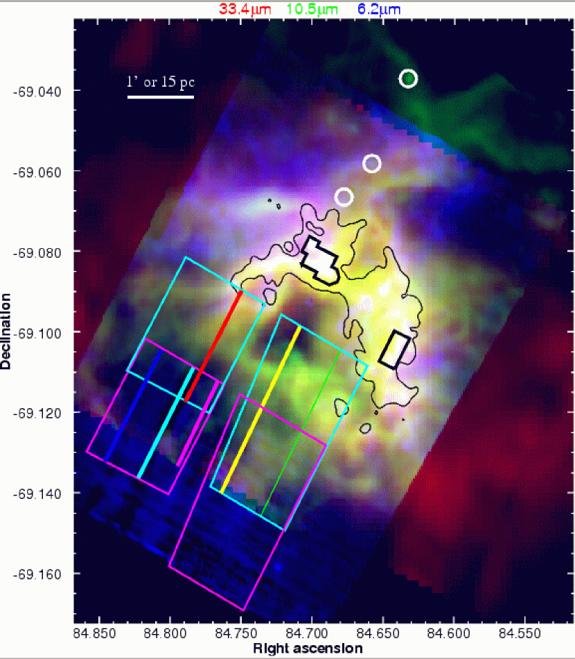
Figure 4: Three-color log-scale image generated from the IRS cube (see §2.1) with regions of interest overlaid. Black contour: a single radio contour to guide the eye (see Figure 2). The emission line maps are continuum-subtracted, and each is plotted at a scale that brings out detail. Red: [S III]$\lambda$33.4$\mu$m, in the LL1 module. Green: [S IV]$\lambda$10.5$\mu$m, in the SL1 module. Blue: PAH at 6.2$\mu$m, in the SL2 module. The areas outlined in bold black are vulnerable to falling response (saturation) and strong fringing in the LL1 module (see Appendix B). Continuum fits in these areas should be regarded with caution, as should the fitted line strengths of long-wave emission lines. The sources marked in white saturated the peak-up camera and caused dark stripes and other artifacts in the SL modules elsewhere in the map. The cyan regions represent the total affected area for the SL1 module, while the magenta regions represent the total affected area for the SL2 module. However, the main effect of the saturation is a stripe across the map that changes with wavelength. There are generally no severe effects in the rest of the map for a given wavelength. The approximate location of this stripe is marked by a series of bold lines, for several wavelengths corresponding to major emission lines in our spectra. Blue: [Ar II]$\lambda$7.0$\mu$m. Cyan: PAH at 6.2$\mu$m. Magenta: Humphreys-$\gamma$ $\lambda$5.90$\mu$m. Green: [Ar III]$\lambda$9.0$\mu$m. Yellow: [S IV]$\lambda$10.5$\mu$m. Red: [Ne II]$\lambda$12.8$\mu$m. See §2.2 for more detailed discussion.

2.3 Spectral Features and Line Fitting

Hot dust emission is responsible for the overall shape of the continuum in 30 Doradus and its strong rise toward the red. Using the fitting package PAHFIT (Smith, 2007a), we fit the continuum with an assortment of four thermal functions from 40 to 300K and a stellar blackbody of 5000K (the fit is insensitive to exact temperature as long as it peaks blueward of our shortest wavelength 5$\mu$m). The integrated spectrum of the entire region is shown below in Figure 5, and astrophysically interesting spectra are described below in §3.3.

The broad PAH bands and unresolved atomic lines are blended in some parts of the spectrum. In order to decompose them, we fit the whole suite of emission lines at once. Detailed analysis of the dust features will be addressed in a future work. The feature of greatest potential concern is blending of [Ne II]$\lambda$12.8$\mu$m with the 12.7$\mu$m PAH feature. The PAH contribution is much lower than the atomic line over much of 30 Doradus. In particular, Sturm et al. (2000) found that at the higher spectral resolution of ISO-SWS, the 12.7$\mu$m PAH feature was undetectable relative to [Ne II]$\lambda$12.8$\mu$m within the two ISO-SWS apertures (located on the ridge) – the lowest ratio of PAH to [Ne II] of any H II region they studied. We used comparisons with high-resolution spectra (see Appendix B) and tests in parts of 30 Doradus that should be completely PAH-free, like the core of R136, to determine that the joint fitting of those two features is robust in 30 Doradus and uncertainties are properly accounted for.

2.4 MIPS SED cube

We also made contemporaneous observations of 30 Doradus using the SED mode of the MIPS (Rieke et al., 2004; Lu et al., 2008). The raw data are responsivity-corrected, dark-subtracted, and illumination-corrected using the MIPS germanium pipeline (Gordon et al., 2007), with the difference that the illumination correction is derived from Galactic cirrus rather than zodiacal light. Wavelength correction is derived from observations of bright planetary nebula. Since 30 Doradus is so bright, we use the chopped “background” area simply as additional on-source observation, and assume that the thermal background is much less intense than the emission from the nebula itself. As with the IRS data, mapping the area with offsets equal to half of the slit width, perpendicular to the slit direction, yields a fully sampled spectral cube, with resolution $\lambda/\delta\lambda\simeq$25. Even with such poor resolution, we detect [N III]$\lambda$57.3$\mu$m with high significance over most of the map, and tentatively [O I]$\lambda$63.1$\mu$m in the very center (§3.1). The shape of the dust continuum will be discussed in a future publication on the dust content of 30 Doradus, but we note that the SED peaks shortward of 75$\mu$m, consistent with very high average dust temperatures (Figure 5).

Figure 5: The spectrum of the entire 30 Doradus nebula (a square about 4’ or 60 pc on a side centered on 05^h38^m44^s -69^∘05′28″). The observed spectra from IRS and MIPS/SED, and infrared photometric points, are plotted with symbols, while the fit we made to the IRS data is displayed with a solid line.

3 Results

Figure 5 shows the integrated spectrum of 30 Doradus, with dust and atomic features labeled. The overall continuum shape is typical of hot small dust grains in H II regions. The MIPS/SED data clearly show that the spectral energy distribution of the entire nebula peaks shortward of 70$\mu$m, indicating a quite warm average dust temperature. A full discussion of dust properties will be the subject of a subsequent publication. We note that the aromatic features are well-detected but not extremely strong - comparable to Galactic compact H II regions or compact blue galaxies, and weaker than the integrated spectra of entire spiral galaxies or the diffuse emission of the Milky Way (Galliano et al., 2008; Peeters et al., 2002). The equivalent width of the 6.2$\mu$m feature, averaged over this large aperture, is 0.61$\mu$m. In particular, the weak 17$\mu$m feature may indicate a dearth of large neutral PAHs (Smith, 2007a) in this intensely ionized environment. The strongest spectral features are the ionic emission lines which are sensitive to physical conditions in the ionized gas.

Table 1: Ionization Potentials.

	I	II	III	IV
O	13.62	35.12	54.94	77.41
Ne	21.56	40.96	63.45	97.11
S	10.36	23.33	34.83	47.30
Ar	15.76	27.63	40.74	59.81

Note. — Units are eV.

In the following sections we describe the spatial distribution of emission lines and their ratios, and show spectra of notable compact regions.

3.1 Spatial distribution of emission

Figures 6-14 show maps of ionic line emission in 30 Doradus. To first order, line emission follows the diffuse emission pattern seen at other wavelengths, of a broad arc or “ridge” surrounding an evacuated hole. The overall excitation of the region is immediately clear from the distribution of [Ar II] and [Ar III] – there is no detected [Ar II] in the evacuated hole. With an ionization potential of 15.7eV, the photoionization cross section and charge transfer with hydrogen ensures very little Ar⁺ within an H II region (e.g. Sofia & Jenkins, 1998). (Ionization potentials are listed in Table 1 for reference.) We note that the Ar⁺⁺ recombination rate is highly uncertain, so absolute calibration of [Ar III]/[Ar II] has large systematic uncertainty (Morisset et al., 2004; Stasińska & Schaerer, 1997). The similarity of overall morphology amongst the Ar, Ne, and S lines suggests that any variation of excitation across the nebula will be correlated with the structure seen in continuum from radio to infrared, although as we will explore thoroughly below, the shape of the hole varies somewhat, and there are some distinct locations of high excitation. The [Si II] distribution appears somewhat displaced away from R136 and the cavity, as would be expected since the line is strong in PDRs as well as ionized gas.

Lower ionization species have tentative detections in a few places, but never very strongly or widely distributed. Of particular interest is a peak near 5^h38^m44.9^s -69^∘05′13″ (source “0”, §3.3), at which we also detect [N III]$\lambda$57.3$\mu$m and [O I]$\lambda$63.1$\mu$m in MIPS SED observations (see the northeastern region marked in Figure 11). The spectra in this part of the map are affected by fringing in the LL1 module ($>$20$\mu$m), so a [Fe II]$\lambda$26.0$\mu$m detection in the same region is considered tentative. The ratios of [Ne III]/[Ne II] and [S IV]/[S III] (and the MIR continuum) are high in this general area, but this region in the center of the ridge is complex, and the higher ionization species do not peak in exactly the same location as these lower ionization species. In fact, the peak of low-ionization species falls between two peaks of the [Ne III]/[Ne II] map.

Molecular hydrogen emission is detected in the central molecular ridge and marginally detected in several other locations. Only the S(3) 9.67$\mu$m line is reliably detected over much of the map. Tentative detections in our low-resolution spectra of the S(0) 28$\mu$m line can be ruled out by examining the handful of high-resolution spectra in 30 Doradus. Detection of the S(2) 12.28$\mu$m line independently of the neighboring Humphreys-$\alpha$ $\lambda$12.37$\mu$m line is not very reliable with low-resolution spectra as described in more detail below, and from the high-resolution spectra we find that the molecular line is weaker than the atomic line everywhere, and less than 15% over most of the central part of the map.

Higher excitation species [O IV] and [Ne V], which have strong lines in the IRS bandpass, are not detected in our maps. As discussed in §5.2, this favors photoionization over shocks as the dominant physical process in the region.

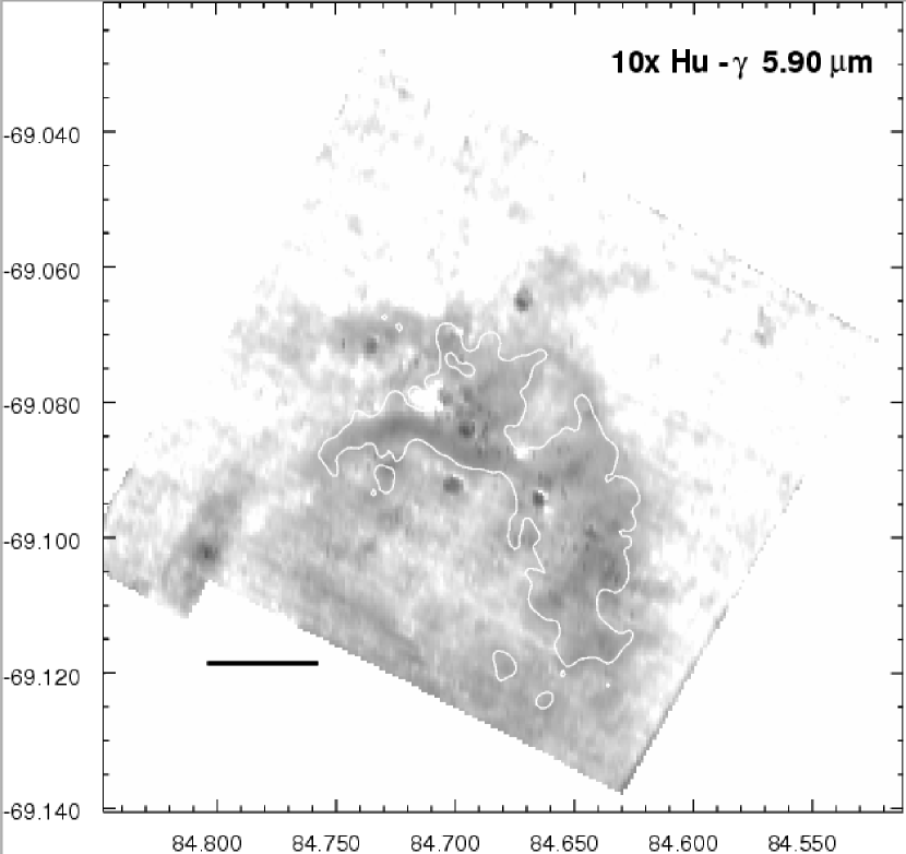
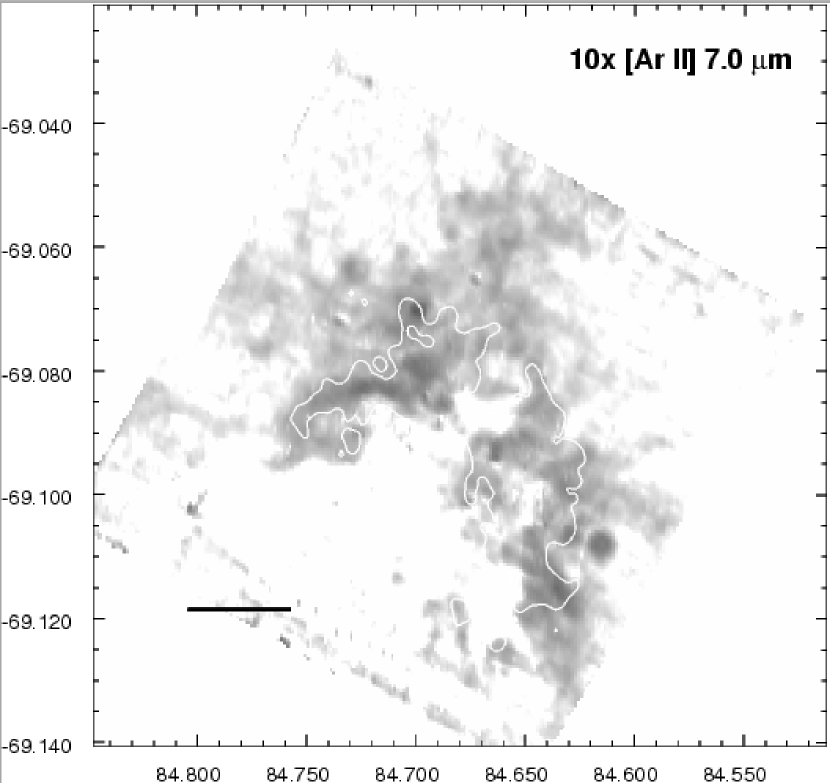
Figure 6: through Figure 11: Fitted atomic line maps. All plots are on the same log scale, ranging from $10^{-7}$ to $10^{-5}$ $Wm^{-2}sr^{-1}$. Note that four of the fainter maps have been multiplied by 10, and the brighter [O III] map has been divided by 100. The length of the black bar is 1” or 15 pc. White contours: a single level of 3cm radio emission, to guide the eye (see Figure 2).

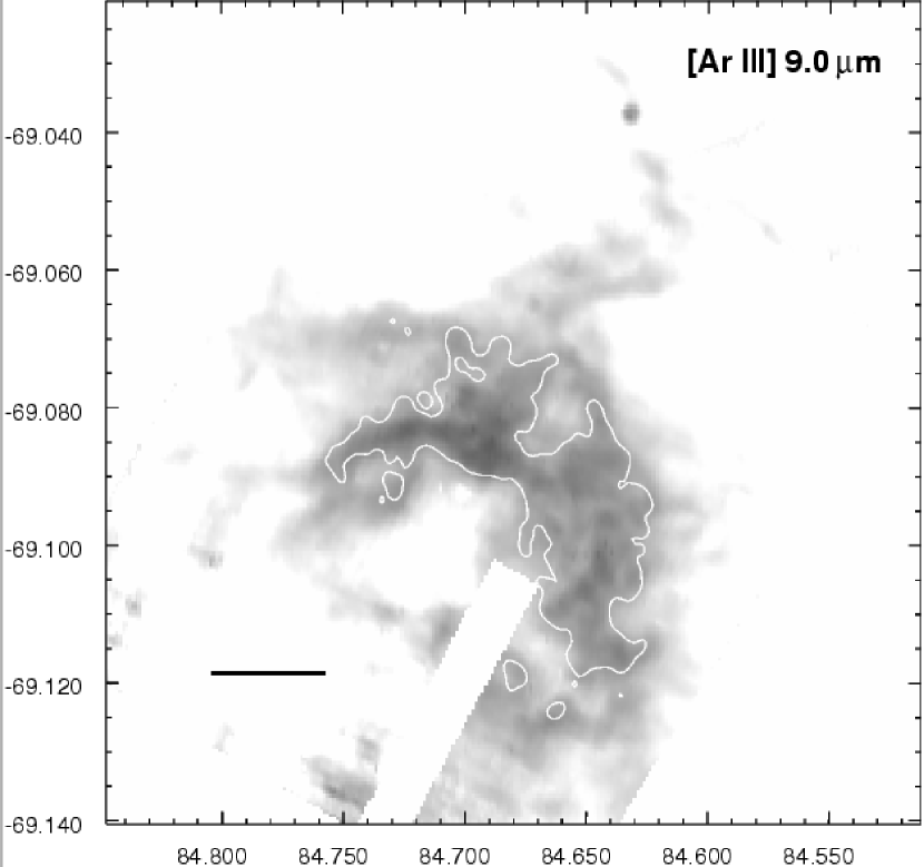
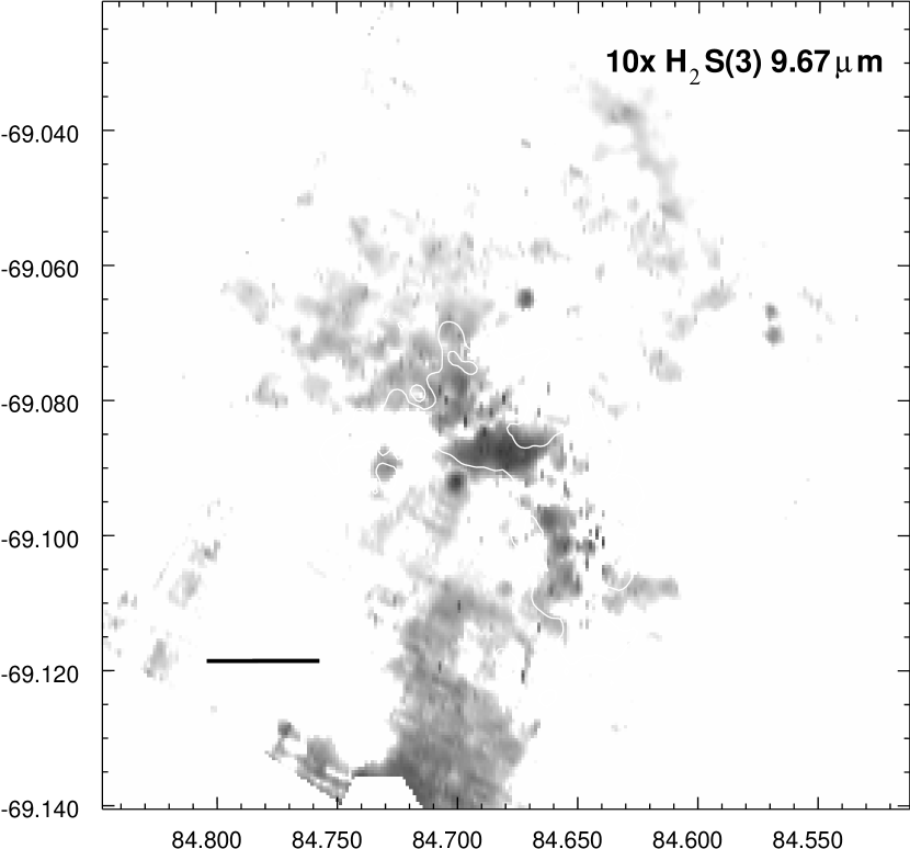
Figure 7: Fitted line maps (see caption, Figure 6).

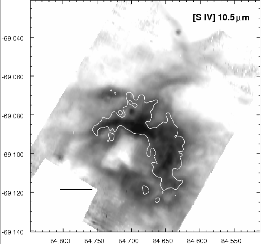
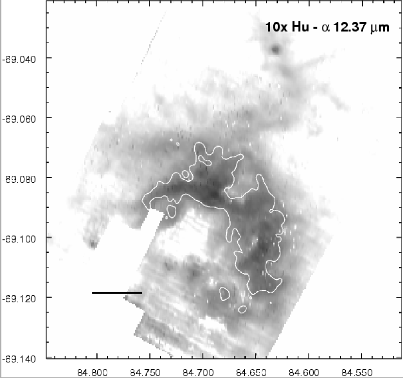
Figure 8: Fitted atomic line maps (see caption, Figure 6).

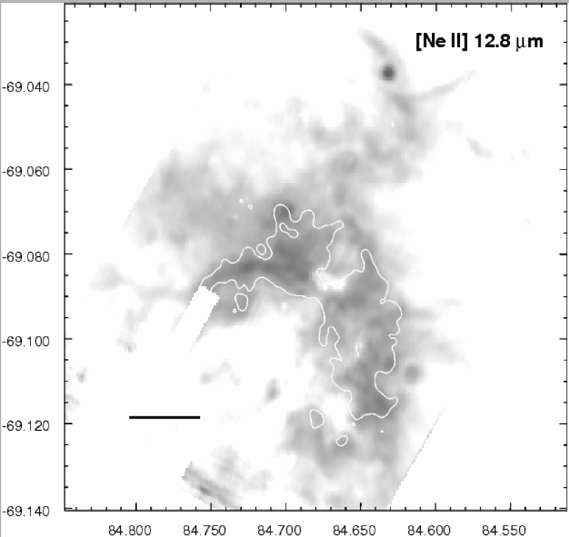
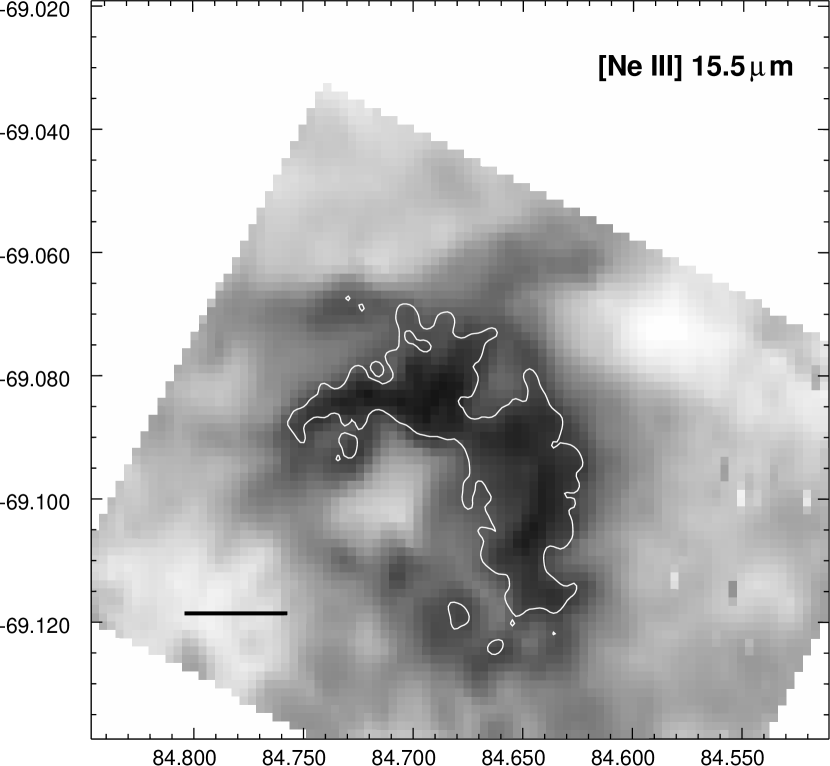
Figure 9: Fitted atomic line maps (see caption, Figure 6).

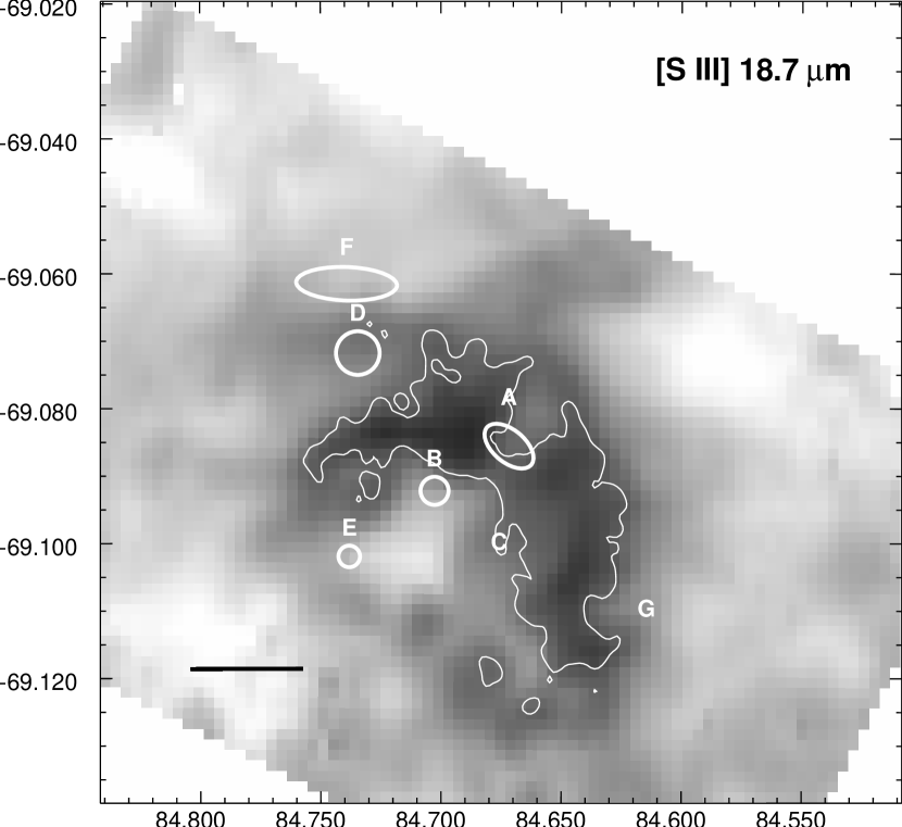
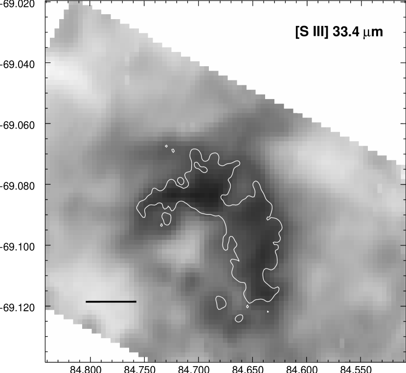
Figure 10: Fitted atomic line maps (see caption, Figure 6). The [S III]$\lambda$18.7$\mu$m map is marked with regions of interest listed in Table 2.

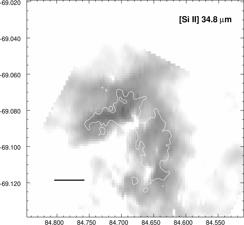
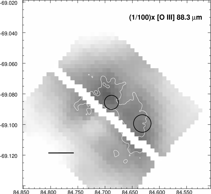
Figure 11: Fitted atomic line maps (see caption, Figure 6). The black circles on the [O III]$\lambda$88.3$\mu$m map mark the detected peaks of [O I]$\lambda$63.1$\mu$m and [N III]$\lambda$57.3$\mu$m.

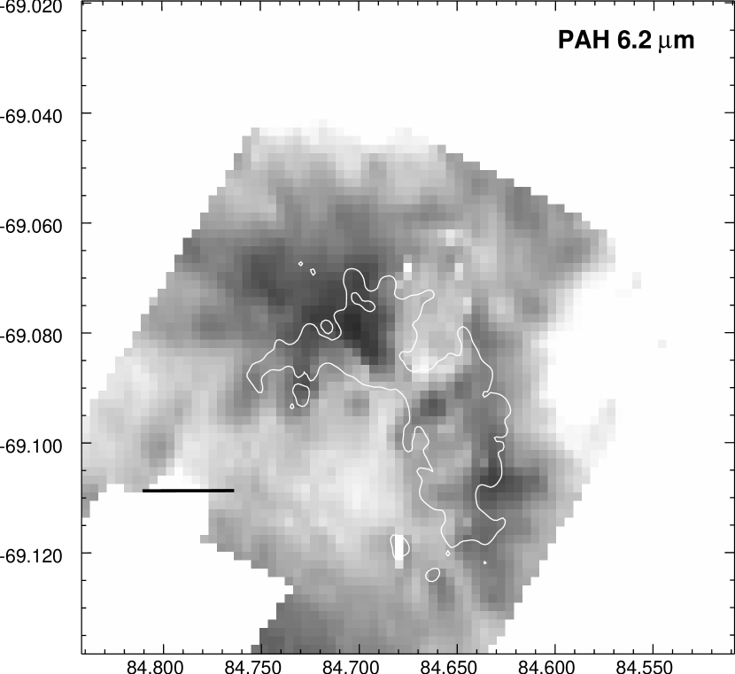
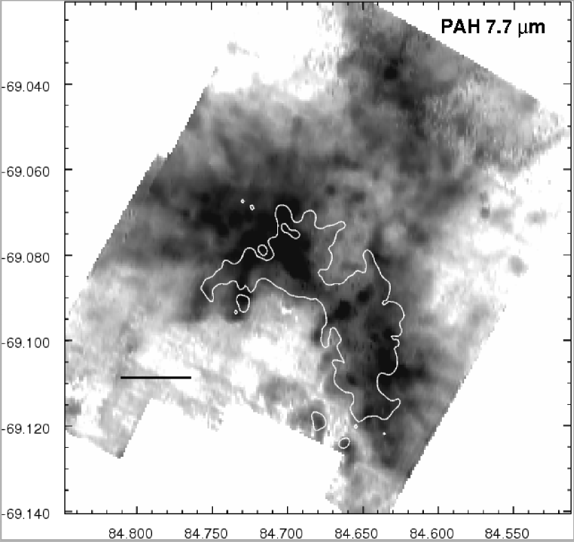
Figure 12: through Figure 14: Fitted PAH feature maps. For details, see caption, Figure 6.

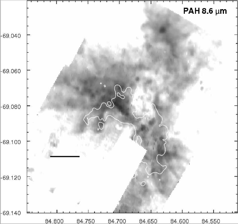
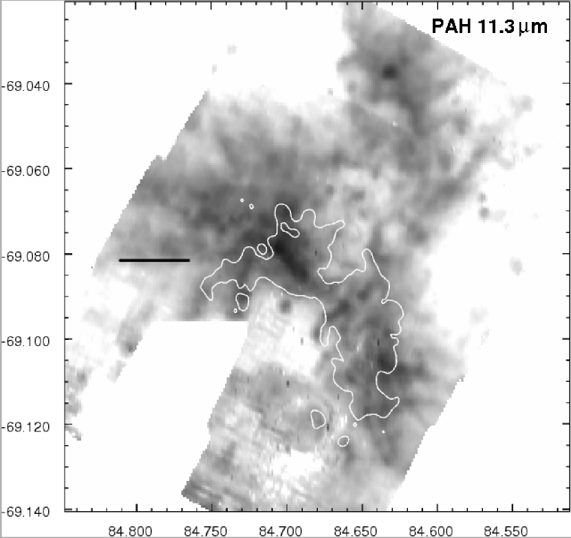
Figure 13: Fitted PAH feature maps (see caption, Figure 6).

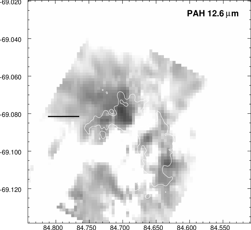
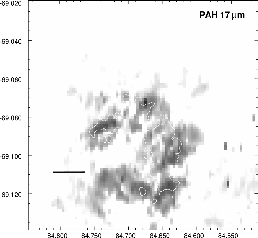
Figure 14: Fitted PAH feature maps (see caption, Figure 6).

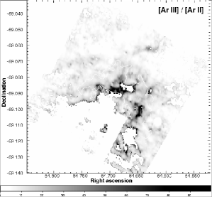
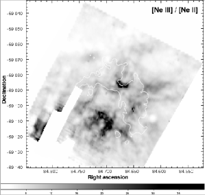
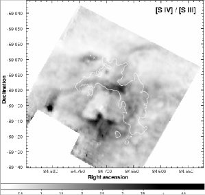
Figure 15: Line ratios on a linear scale. White contours: a single level of 3cm radio emission, to guide the eye (see Figure 2). The white region in the middle of the argon ratio plot indicates nondetection of [Ar II]$\lambda$7.0$\mu$m and a very high value of the ratio. Small masked regions in the lower left of the plots are affected by artifacts (see Fig. 4).

3.2 Line Ratios

Figure 15 shows the three line ratio maps [Ar III]$\lambda$9.0$\mu$m/ [Ar II]$\lambda$7.0$\mu$m, [Ne III]$\lambda$15.5$\mu$m/ [Ne II]$\lambda$12.8$\mu$m, and [S IV]$\lambda$10.5$\mu$m/ [S III]$\lambda$33.4$\mu$m. These species all have ionization potentials above 13.6eV, and thus are sensitive to the shape or hardness of the ionizing spectrum (we will call this $T_{rad}$, because it is often parameterized by the temperature of the best-fitting black-body over $\lambda<$912Å) and the intensity of ionizing radiation. The latter is usually quantified as the dimensionless ionization parameter

$$U={1\over{n}}\int_{13.6eV}^{\infty}{{F_{\nu}}\over{ch\nu}}d\nu,$$

or ratio of ionizing photon density to atom density. Any single line ratio cannot distinguish between elevated $U$ or $T_{rad}$, but because the spacing of the ionization potentials differs with atom, different ratios have different $U$ and $T_{rad}$ dependencies, and measuring two ratios can break the degeneracy. (This has been discussed by many authors, see especially the discussions in Morisset et al., 2004; Martín-Hernández et al., 2002; Dopita et al., 2006, ,and §5.1 and Fig 20 below.).

All ratios increase with $U$, but locations where the ratios are not well correlated can indicate changes in the hardness of the ionizing field. In 30 Doradus the ratios are very well correlated (correlation coefficient of 0.7 between the neon ratio and argon ratio map, 0.8 between the neon and sulphur ratios, and 0.7 between the argon and sulphur ratios). The Ne and S ratios are telling us similar things over much of the region. For example, there is high excitation in a “hot spot” between the two lobes of the ridge (source “A”, §3.3), and in the region to the south of the bubble. There is a low excitation ridge to the north (source “F”, §3.3). The location noted above for low argon emission (source “G”, §3.3) is significantly low in all three line ratios.

Interestingly, the Ne and S line ratios show quite different behavior on the eastern edge of the bubble, where [Ne III]/[Ne II] is high but [S IV]/[S III] is low (the red region in Figure 21 below, centered on source “E”, §3.3). The S ratio is more affected by extinction since [S IV]$\lambda$10.5$\mu$m is in the silicate dust absorption feature, so that could be a region of very high extinction or a region of particularly hard ionizing radiation. In this case, the sulphur ratio does not vary dramatically throughout the bubble, and it is the neon ratio which is higher at the western end, which argues for harder ionizing radiation. An extinction effect would require simultaneous increase in the ionization parameter or strength of the ionizing field and increased extinction. The specific extinction difference (A([S IV]$\lambda$10.5$\mu$m)-A([S III]$\lambda$18.7$\mu$m))/A(2.1$\mu$m) equals 0.42$\pm$0.03 (uncertainty reflects differences between published extinction curves; we used that in PAHFIT, Smith, 2007a), whereas the effect of extinction on the neon ratio is small (A([Ne III]$\lambda$15.5$\mu$m)-A([Ne II]$\lambda$12.8$\mu$m))/A(2.1$\mu$m) = 0.0$\pm$0.07. Reproducing the observed line ratios without changing the hardness of the ionizing field would require A(2$\mu$m)$\simeq$0.75, or A${}_{V}\simeq$6. Such significant extinction seems unlikely given the overall relatively low extinction in the region, and is not detected in our extinction maps (§4.1).

One question that is possible to investigate with this dataset is whether the optically known hot stars in 30 Doradus can completely account for the ionization structure, or whether embedded star formation affects gas excitation measured in the infrared that otherwise might be concealed by at other wavelengths. On Figure 16 we plot show the location of Wolf-Rayet stars and early O stars (there are discrepancies between spectral types determined by different authors, and our intent is to show the most massive stars, not provide the most precise spectral typing possible). There is a cluster of WR stars between the two lobes of the ridge, coincident with very high excitation gas. There is not a dramatic increase of excitation centered on R136, although the excitation is generally high in the area. Figure 16 also shows the 3.5$\mu$m-excess sources of Maercker & Burton (2005), representing a crude selection of possible protostellar candidates. Other kinds of sources, including some of the previously identified WR stars, can also display infrared excess. Nevertheless, this selection of sources does trace what is known from more precise studies with incomplete spatial coverage (e.g. Rubio et al., 1998; Brandner et al., 2001), that the young embedded sources in this region are concentrated along the IR-bright ridge. The protostellar candidates shown here do not show any particularly striking correlation with regions of high excitation – in fact the southern part of the region has high excitation and few protostellar candidates. We conclude that the ionization structure in 30 Doradus is primarily determined by the (optically) known hot stars.

Figure 16: IRAC 8$\mu$m image (log scale) with two types of relevant point sources: Circles show the most energetic stars in the region - Wolf-Rayet stars and early O stars, from Breysacher et al. (1999); Parker (1993), and X’s show protostellar candidates determined from 3$\mu$m excess emission by Maercker & Burton (2005). White contours: a single level of 3cm radio emission, to guide the eye (see Figure 2).

3.3 Notable Regions

Figure 17 shows the spectra of small regions which stand out in the continuum (Fig 1), in the feature maps (Figures 6 through 14), or in the line ratio maps (Fig 15). They have been chosen to illustrate the range of excitation, extinction, and continuum shape in the 30 Doradus nebula. These regions of interest were marked on Figure 2, and are listed for reference in Table 2.

Figure 17: Spectra of the seven regions described in §3.3, with errorbars. For comparison, the spectrum of the entire region (Fig 5) is repeated at the top, with feature labels.

Table 2: Notable Sources

label	RA	Dec	description
“0”	5h38m45s	-69d05m13s	brightest point on ridge
“A”	5h38m42s	-69d05m05s	hot spots between molecular clouds
“B”	5h38m49s	-69d05m32s	Parker (1993) #1445 MI star
“C”	5h38m42s	-69d06m00s	R136
“D”	5h38m56s	-69d04m18s	example of high extinction
“E”	5h38m57s	-69d06m07s	isolated WN6 star R145
“F”	5h38m57s	-69d03m42s	low-excitation trough
“G”	5h38m28s	-69d06m30s	SW low-excitation region

Source “0” is the brightest point on the ridge in most tracers, including infrared continuum, many lines, and centimeter continuum. We detect [N III]$\lambda$57.3$\mu$m and [O I]$\lambda$63.1$\mu$m in MIPS SED observations at this location, and tentatively [Fe II]$\lambda$26.0$\mu$m, although this small region of the map is affected by residual fringing and saturation in the LL1 module, raising the uncertainty of the [Fe II]$\lambda$26.0$\mu$m detection.

Source “A” is a diffuse region between the two lobes of the molecular ridge. We describe it as a “hot spot” because it has locally elevated excitation seen in the line ratios (Fig 15), and when analyzed with photoionization models, is best fit with a hotter or harder radiation field (Fig 21, §5.1). There are known hot stars in the vicinity, but it is not completely clear if they are responsible for the locally higher excitation in the H II region.

Source “B” is a prominent point source from optical to MIR wavelengths, and has been spectroscopically classified as an M supergiant Parker (1993, ; see also refs therein). Their quoted absolute V magnitude appears to place the star at twice the distance to the LMC, but other authors note that it is likely in the foreground. It seems unlikely in any case that it is located in the bubble or affecting the ionization structure. Because this source exhibits silicate emission at 9.8 and 18 $\mu$m rather than absorption, PAHFIT cannot be applied to it using the parameters used on the rest of the spectral cube. It is the only source in Figure 17 without the fitted spectrum overlaid on the data points and errorbars.

Source “C” is the R136 cluster core.

Source “D” is a prominent mid-infrared point source outside the main cluster and bubble. The surrounding ionized gas has quite high atomic line ratios and thus appears quite highly excited, but we were unable to find a hot star cataloged in the literature which might be responsible for this local excitation. This region also shows relatively high extinction compared to the rest of 30 Doradus. Extinction can raise the sulphur line ratio but has relatively small effect on the neon line ratio, so in our opinion the extinction is not responsible for the apparently high excitation.

Source “E” is a known WN6 star R145, fairly isolated from other catalogue hot stars at the eastern end of the bubble. The high fitted radiation temperatures in the neighborhood of this source (§5.1) are consistent with excitation by the harder expected radiation field from a Wolf-Rayet star.

Source “F” is an east-west extended region that appears to be a trough or low point in the excitation and line ratios. The electron density is not remarkable, neither does there appear to be any molecular gas traced by CO emission in the vicinity. It is possible that the feature is in the foreground of this three-dimensional nebula.

Source “G” is a region associated with two peaks in the CO emission [JGB98] 30 Dor-12 and 13 (Johansson et al., 1998), just to the west of the main ridge. There is a peak in both argon line maps at this location, and the region is a low point in all three excitation ratios [Ar III]/[Ar II], [Ne III]/[Ne II] and [S IV]/[S III]. There are in fact several discrete parsec-sized regions of low excitation in the vicinity There is little 3cm continuum at those locations, which lie almost exactly on the opposite side of a molecular cloud from R136. One spot coincides with a knot in the infrared diffuse continuum (#29) noted by Hyland et al. (1992). There is a 3.5$\mu$m-excess protostellar candidate (Maercker & Burton, 2005, and Fig. 16) nearby, but not coincident with the low-excitation spots. High resolution and sensitivity molecular observations may reveal dense, starless molecular clumps in this part of 30 Doradus, (self)-shielded from the intense radiation.

4 Distribution of Matter: Extinction and n_e

4.1 Extinction

Previous estimates of the extinction in 30 Doradus found A_V=1.1$\pm$0.1$mag$ (Dickel et al., 1994, and refs therein), with two possible locations of higher extinction at 05^h38^m39^s -69^∘07′30″ and 05^h38^m32^s -69^∘06′22″. Rosa & Mathis (1987) found extinction corrections at H$\beta$ of 0.5-1.0 (A_V=0.4-0.8) at ten locations in the outer parts of the region we are studying. We make three estimates of extinction in the region, two directly from our dataset. All methods suffer from systematic uncertainty and modest signal-to-noise, but we can be confident of higher extinction in the regions that all three methods agree.

First we use the ratio of centimeter continuum to H$\alpha$ emission to derive a map of extinction in 30 Doradus, following the procedure used in Lazendic et al. (2003) and using their centimeter data that they kindly provided (magenta contours, in Fig. 18). We assume that all of the centimeter continuum emission in the 30 Doradus region is thermal. Single dish measurements estimated that the nonthermal component contributes less than 2% at 6cm (Shaver et al., 1983, and refs therein). Lazendic et al. (2003) identified two possible supernova remnants from comparison of cm synthesis images and optical recombination lines, but their own analysis and subsequent followup with optical and Xray imaging and optical spectroscopy suggests that these are merely extinguished H II regions (Chu et al., 2004). The relationship between thermal bremsstrahlung centimeter continuum and hydrogen recombination line emission depends weakly on the electron temperature, but Rosa & Mathis (1987) and Peck et al. (1997) both found that T_e variations are small in 30 Doradus ($\lesssim\pm$300K), so it is unlikely that the calculated extinction variations are actually misinterpreted T_e variations.

We derived two more maps of extinction directly from the IRS spectral cube. Amorphous silicate dust is responsible for two broad bands of absorption at 9.7 and 18$\mu$m. The PAHFIT package reports the fitted optical depth at 9.7 $\mu$m. The resulting map for 30 Doradus is shown in Figure 18, in green contours. The fit to the absorption feature is sensitive to noise in the spectrum. We cropped away southern parts of the map that were clearly artifacts, and any part of the map where the signal-to-noise was less than 2. Finally, we median-smoothed the resulting map with a window of 3 pixels. The result is a sparse map showing the regions of comparatively reliable elevated silicate absorption.

The ratio of Hydrogen recombination line strengths can also be used to calculate extinction, most commonly by assuming an intrinsic (unextincted) ratio from Case B recombination. Our dataset includes Humphreys-$\alpha$ (7-6) and Humphreys-$\gamma$ (9-6). Due to modest signal-to-noise and to a systematic tendency of PAHFIT to slightly underestimate the continuum level near these wavelengths, the absolute value of extinction calculated from this ratio has a large systematic uncertainty. It is also difficult to resolve the weak Humphreys-$\alpha$ line from H₂ S(2) 12.28$\mu$m in low-resolution spectra. We quantified the amount of potential contamination to the Humphreys-$\alpha$ line strength in several ways: We fit our low-resolution spectra with and without the molecular hydrogen line (the central wavelengths of both lines are very tightly constrained by PAHFIT), and found that the Humphreys-$\alpha$ line strength was only decreased by 15% (that flux was attributed to H₂) when both lines were included. We also fit the high-resolution GTO spectra, in which the lines are easily separated and reliably measured, and found that over most of our area, H₂ was less than 20% of Humphreys-$\alpha$. We examined fits to both the high and low-resolution spectra in the few high-resolution apertures where the H₂ and Humphreys-$\alpha$ strengths are comparable (H₂ never exceeds Humphreys-$\alpha$ in strength) and found that the low-resolution Humphreys-$\alpha$ strength used in our analysis was at most overestimated by 40% by the presence of the H₂ line on the wing of the Humphreys-$\alpha$ line. While some level of contamination of Humphreys-$\alpha$ by H₂ S(2) may be present in our maps, we do not expect that to change any of our conclusions including the regions of high extinction identified in Figure 18.

Further systematic uncertainty arises in the choice of extinction curve, since the lines lie on the wings of the silicate absorption features, which vary in amplitude and width in different studies. However, all extinction curves that we considered show greater relative extinction at Humphreys-$\alpha$ $\lambda$12.37$\mu$m than at Humphreys-$\gamma$ $\lambda$5.90$\mu$m. We examined the extinction curves of Chiar & Tielens (2006) for the Galactic Center and the ISM, and the average LMC extinction curve based on the carbonaceous-silicate grain model of Weingartner & Draine (2001). All of the extinction curves roughly agree in the vicinity of the Humphreys-$\alpha$ emission line. Near the Humphreys-$\gamma$ line, the Chiar & Tielens curves agree well with the near-infrared extinction for the ISM found by Indebetouw et al. (2005). Thus, extinction correlates with the flux ratio of Humphreys-$\gamma$ $\lambda$5.90$\mu$m to Humphreys-$\alpha$ $\lambda$12.37$\mu$m, and we can still find the relative level of extinction across 30 Doradus from the Humphreys-$\alpha$/Humphreys-$\gamma$ ratio, even though the absolute normalization is uncertain.

We calculated the signal-to-noise of the ratio based on the RMS variance of the individual maps of emission line strength, and removed all regions of the map where the signal-to-noise was less than 2. We cropped away the parts of the map where an additive correction was made to the SL spectra (see §A.0.3), because this subset of the map encloses some spectra which have an unphysical plunge at the red edge of the SL2 module. The fit to those spectra generally underestimates the continuum near the Humphreys-$\gamma$ line, and thus overestimates the ratio of Humphreys-$\gamma$ to Humphreys-$\alpha$. We also cropped away the parts of the map where the reduced $\chi^{2}$ of the fit was greater than 5. Finally, even after applying these filters, it was necessary to trim away some regions from the low-signal edge of the map where the noise levels were still untrustworthy. The ratio map shown in grayscale in Figure 18 is now mainly limited to those areas of 30 Doradus where we obtained both good detections of these two faint lines and a good fit.

Despite the level of noise in the maps of extinction, particularly the map derived from the Humphreys-$\alpha$ and Humphreys-$\gamma$ lines, there are three areas where all three methods agree on especially high extinction. These areas have been marked on Figure 18. Generally, there is not much extinction by dust in 30 Doradus. As discussed above, extinction has a small effect on the Neon excitation ratio, but raises the [S IV]/[S III] (due to the shape of the extinction curve), which in turn will get interpreted as higher T_rad in our photoionization models. The regions of interestingly high T_rad do not turn out to correspond to regions of clearly high extinction, but the effect should be kept in mind in interpreting the data.

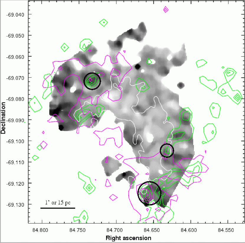
Figure 18: Map of extinction in 30 Doradus. Grayscale linear image: the IRS Humphreys-$\gamma$/Humphreys-$\alpha$ ratio, which is proportional to extinction. Dark areas of the map indicate high extinction. The Humphreys lines are weak, and this map has been severely cropped to remove areas of the worst signal-to-noise. Green contours: the optical depth of silicate absorption from the IRS spectral map, $\tau=0.10,0.27,0.43,0.60$. Areas of low signal-to-noise have been masked out of this map as well. Magenta contours: The ratio of the 3cm continuum (Lazendic et al., 2003) to H$\alpha$ emission (MCELS, http://www.ctio.noao.edu/$\sim$mcels/), also proportional to attenuation. The northernmost magenta source corresponds with the molecular cloud marked in yellow in Figure  1. White contours: a single level of 3cm radio emission, to guide the eye (see Figure 2). The areas where all three maps tend to agree on high extinction have been marked in black. The northeasternmost corresponds with source “D” in Figure 2 and §3.3.

4.2 Electron Density

Figure 19 shows the electron density calculated from [S III]$\lambda$18.7$\mu$m/[S III]$\lambda$33.4$\mu$m. The [S III]$\lambda$18.7$\mu$m map was convolved to the lower resolution of the [S III]$\lambda$33.4$\mu$m map, and the line ratio converted to electron density using the conversion in Dudik et al. (2007) at $T_{e}$=10⁴K (their Figure 9 and section 6: Those authors calculated the line ratio as a function of density and temperature for a five level atom using the collision strengths from Tayal & Gupta (1999) and radiative transition probabilities from Mendoza & Zeippen (1982)). The calculated ratio is not a strong function of temperature. The ridge is prominent in the [S III] ratio or n_e map, and in fact the n_e map is quite similar to the 3cm continuum in morphology. The density is elevated to the south of the bubble and R136, in a region of relatively high excitation.

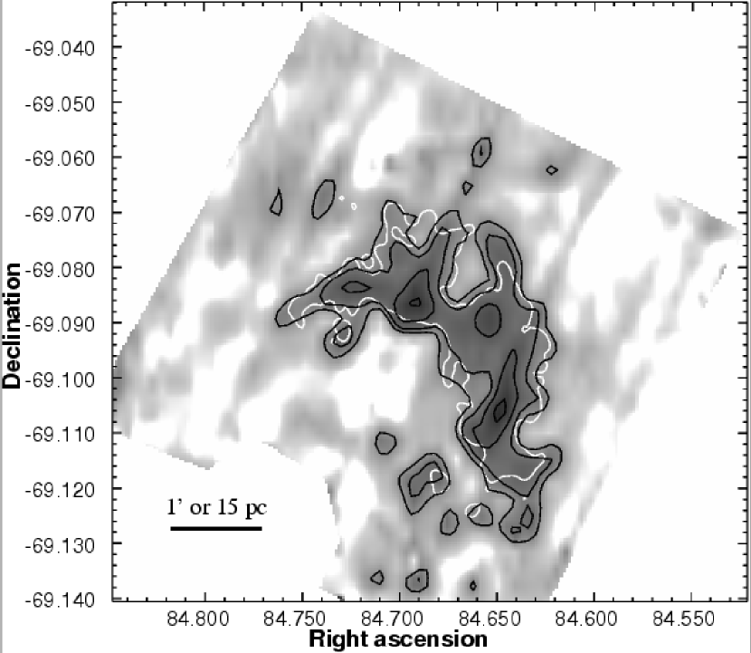
Figure 19: n_e calculated from [S III]$\lambda$18.7$\mu$m/[S III]$\lambda$33.4$\mu$m. Black contours: log n_e = 2.4, 2.5, 2.6, 2.7. White contour: a single level of 3cm radio emission (see Figure 2). The ridge is prominent, as well as a region of increased density to the south.

4.3 Abundances

Variations in elemental abundances can in principle change the diagnostic ratios that we are using to measure physical conditions in the 30 Doradus nebula. Previous studies have found very small internal abundance variations in 30 Doradus and other giant H II regions. Peck et al. (1997) found no significant variations on 15″ scales in the He abundance $Y^{+}=He^{+}/H^{+}$ = 0.13$\pm$0.02 measured from radio recombination lines. Rosa & Mathis (1987) found little variation between several positions measured with optical spectroscopy. Of more direct relevance to this work, Lebouteiller et al. (2007) found less than 0.01 dex dispersion of Ne/H, S/H, and Ar/H, using the high resolution GTO Spitzer spectra mentioned above.

Small scale abundance variations in H II regions including 30 Doradus (Tsamis & Péquignot, 2005) have been proposed to explain discrepancies between optical and infrared abundance determinations. We might hope to detect sub-parsec scale abundance variations in this dataset by using three infrared line ratios to solve simultaneously for $U$, $T_{rad}$, and $Z$. In practice, we find that the excitation variations can be adequately explained without abundance variations, which would be seen as residuals in our fitting of $U$ and $T_{rad}$. The signal-to-noise especially in our argon line ratio is insufficient to detect abundance variations at the 0.1 dex level predicted by Tsamis & Péquignot (2005).

Overall, abundances in 30 Doradus are not particularly low: Rosa & Mathis (1987) found Ne/O, S/O, and Ar/O ratios close to solar. Lebouteiller et al. (2007) found Ne/H and Ar/H of 12+log(X/H)=7.76$\pm$0.02 and 6.32$\pm$0.06, respectively, within 0.25 dex of the range of solar values (Lodders, 2007, 2003; Asplund et al., 2005). They found S/H of 6.77$\pm$0.03, only about 0.3 dex sub-solar. We also find that on average, half-solar abundances result in modestly better agreement between the three infrared line ratios in our photoionization models than solar or 0.1-solar models. In practice, systematic effects such as the argon recombination rate have a larger effect on this agreement than the abundances (Morisset et al., 2004; Stasińska & Schaerer, 1997).

5 Distribution of Radiation and Gas: Excitation

5.1 Photoionization models

As mentioned above, if photoionization is assumed to be the dominant physical process, the ionic line ratios depend on $U$, $T_{rad}$, and to a lesser degree metallicity. If one assumes constant abundances and hardness or $T_{rad}$, then the line ratio maps in Figure 15 are maps of the ionization parameter $U$, varying from log $U\simeq$-3 to log $U\simeq$-1.5.

A somewhat more sophisticated analysis is to solve for $T_{rad}$ and $U$ simultaneously. We prepared a grid of photoionization models using Cloudy (Ferland et al., 1998) as a 0-dimensional tool to solve for the ionization structure and line emissivities given a specified radiation field and ionization parameter (we used the output of the first zone in each simulation). We explored different input spectra, including ATLAS (Castelli & Kurucz, 2004), Tlusty (Hubeny & Lanz, 1995), CoStar OB and Wolf-Rayet atmospheres (Schaerer & de Koter, 1997; Smith et al., 2002), and black-bodies. In the end we used a grid of Tlusty atmospheres calculated at half-solar metallicity, extrapolated to hotter effective temperatures using black-body atmospheres to set the functional dependence of line ratios on effective temperature, and normalizing the ratios to those of the hottest Tlusty models. (We found that adopting different stellar atmospheres primarily changes the line ratios by a constant multiplicative factor, and has very little effect on the functional dependence of the line ratios on effective temperature and ionization parameter.) We were not able to find freely available grids of more modern atmospheres (e.g. WMBASIC, CoStar) at subsolar metallicity, but we performed careful comparisons of our modeling at solar metallicity to understand the systematic effects. If nebular abundances are set at solar levels in the photoionization models, and stellar atmospheres calculated at solar abundance are used for self-consistency, the derived ionization parameter $U$ decreases systematically by about 0.1 dex, and the derived radiation temperature increases systematically by 10%. At solar metallicity, WMBASIC atmospheres result in about a factor of two lower [Ne III]/[Ne II]ratio and a 50% lower [S IV]/[S III]ratio. That would increase the derived ionization parameter in 30 Doradus systematically by $\sim$0.15 dex, and lower the derived radiation temperature by 5–10%. These effects have been explained in detail by other authors, especially Morisset et al. (2004). None of the changes in stellar atmospheres or metallicity that we explored would result in qualitative changes in our conclusions, merely small systematic shifts in derived parameters. We also varied the dust prescription in terms of abundance and grain size. Neither had a strong effect on the line ratios as a function of $T_{rad}$ and $U$, provided that $U$ was calculated locally, i.e. from integrating the diffuse ionizing field in the simulation above 1 Ry, rather than assuming some geometry-dependent expression such as $N_{\star}/c4\pi r^{2}n_{e}$.

Figure 20 shows typical behavior - each measured ratio defines a curve in $U-T_{rad}$ space, but the lines have different slopes because the ionization potentials are spaced differently for the different atoms. This is equivalent to the nearly parallel arrows for $U$ and $T_{rad}$ in Morisset et al. (2004) (see also Martín-Hernández et al., 2002; Dopita et al., 2006). Two measured ratios can better constrain $U$ and $T_{rad}$. We will focus on the Ne and S ratios since [Ar II] is not detected over large parts of the H II region.

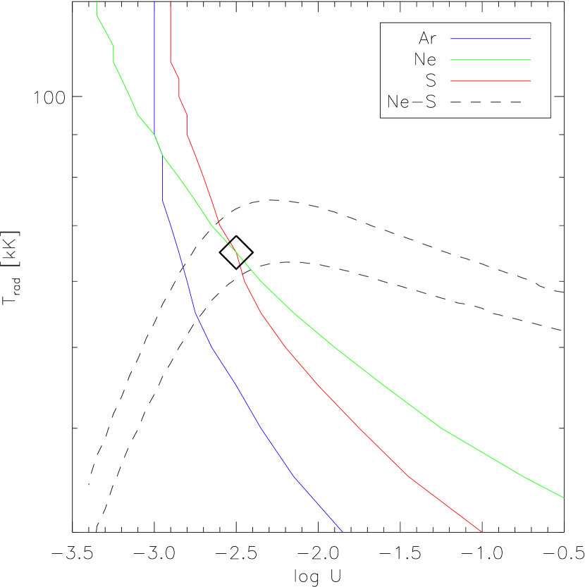
Figure 20: Fits to $U$ and $T_{rad}$ at a representative location 05^h38^m37^s -69^∘06′12″. Loci of consistency with the data are shown for fitting Ar, Ne, and S ratios alone (lines from upper left to lower right), the difference between the S and Ne ratios (log([S IV]/[S III])-log([Ne III]/[Ne II]), dashed lines, 1-sigma confidence interval shown), and the combination of all ratios (bold diamond). See text §5.1 for discussion.

Figure 21 shows the fitted $U$ and $T_{rad}$ across 30 Doradus. The ridge is a region of high ionization parameter, as previously noted from simple examination of the line ratios. The region around the relatively isolated source at 5^h38^m56.5^s -69^∘04′17″ to the north of the ridge is also highly excited, probably due to the local effects of that star (source “D”, Figure 2, §3.3). We note two regions of high $U$ in particular. The most prominent is between the two parts of the ridge (just south of source “A”, §3.3), where young stars may be locally ionizing the gas and beginning to lower the density and disperse the ridge (see Figure 16 for the location of protostars and the most energetic optically identified stars). Alternately, the density is simply lower there and ionizing radiation can more easily leak out from the bubble region around R136. The northern side of this “hot spot” shows evidence for hardening of the radiation field, which could result of the radiation originates in the bubble or on its rim, and is propagating northward, and being absorbed by gas and dust (both of which will harden the field). The high degree of porosity and mixing between molecular and ionized material in 30 Doradus is well known (see e.g. Poglitsch et al., 1995). On the south side of the bubble is another region of high ionization parameter - this region also shows high electron density in the [S III] ratio, so the field must be locally strengthened, perhaps by the WR stars known in that region (Fig 16). Particularly interesting is the region on the eastern side of the bubble, which shows up in the fitted parameter maps as high $T_{rad}$, but not particularly high $U$. There is a single catalogued Wolf-Rayet star (R145, WN6 type, source “E”, §3.3) in the center of that area, which may be energizing the eastern end of the bubble.

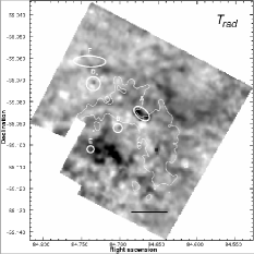
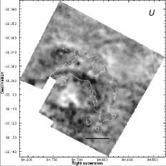
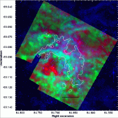
Figure 21: Top: fitted $T_{rad}$ based on the S and Ne line ratios. Middle: fitted $U$. Higher values are dark in both grayscale images. Bottom: fitted $T_{rad}$ (red) and $U$ (green), plus optical B band (blue). All images are in log space except for the B band map. White contours: a single level of 3cm radio emission (see Figure 2). The black lines indicate a scale of 1’ or 15 pc. Sources of interest (see Table 2) are labeled on the $T_{rad}$ map. The derived parameters, $T_{rad}$ and $U$, should be compared with the ratio maps in Figure 15.

The radial variation of physical conditions in 30 Doradus, as a function of distance from R136, is of particular interest, to determine whether feedback in the nebula is dominated by that cluster core, or whether individual hot stars scattered throughout the region are equally important. We have already seen that the latter is true, for example the hot eastern end of the bubble apparently excited by the WN6 star source “E”. Within several tens of parsecs from R136, however, there does appear to be a global effect. The top panel of Figure 22 shows the radial dependence of the ionic line ratios and fitted $T_{rad}$ and $U$. The bubble at $\sim$10pc radius is clearly evident in lowered $T_{rad}$ and raised $U$. Outside the bubble there is a modest gradient in the hardness of the fitted radiation field, but not much gradient in the ionization parameter $U$. This is sensible in a region which has the hottest stars in the center, but some ionizing sources distributed more widely. As R136 is apparently driving an off-center “blister” type H II region, it is interesting to separate the radial dependencies of the ionized gas parameters in the eastern and western direction. The second panel of Figure 22 shows this comparison, showing clearly the bubble wall at $\sim$5pc distance in the east, and the hot bubble between R136 and the $\sim$25pc distant bubble wall in the west. Unfortunately the effects of saturation make the measurements less reliable beyond the bubble wall in the west (see §2.2).

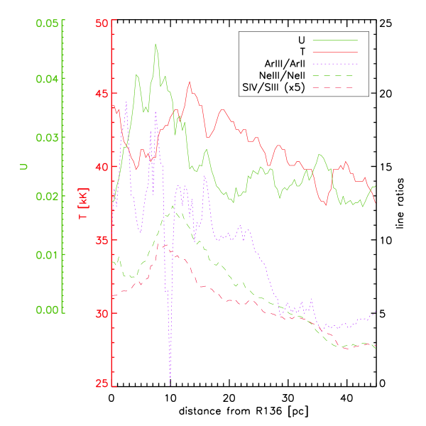
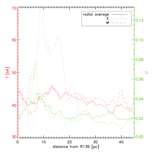
Figure 22: (top) Radial dependence of conditions in the ionized gas as a function of radial distance from R136. The different lines show azimuthal median values of the ionic line ratios and of the fitted $T_{rad}$ and $U$ from photoionization models. (bottom) Radial parameters in the eastern and western directions. R136 is an off-center blister H II region, much closer to the bubble wall in the eastern than western direction.

5.2 Shock Models

Protostellar shocks can also produce MIR fine-structure emission, but only if the excitation (shock velocity) is high enough. [Ne II] requires J-shocks with v$\gtrsim$60km s^-1 (Hollenbach & McKee, 1989) and [Ne III] velocities in excess of 100km s^-1 (Molinari & Noriega-Crespo, 2002). Lefloch et al. (2003) detect [Ne II]$\lambda$12.8$\mu$m and [Ne III]$\lambda$15.5$\mu$m in HH 2, but only from the highest excitation working surface. Similar results are being found with Spitzer, detecting [Ne II]$\lambda$12.8$\mu$m but not [Ne III]$\lambda$15.5$\mu$m, and [S III]$\lambda$33.4$\mu$m but not [S IV]$\lambda$10.5$\mu$m in HH46/47 (Noriega-Crespo et al., 2004), Cep E (Noriega-Crespo et al., 2004), and HH7-11 and 54 (Neufeld et al., 2006). Even the bow shock near a runaway O9.5 star (France et al., 2007) and the stronger shocks in SNR (Neufeld et al., 2007) show similar relatively low-excitation MIR emission.

The (few) MIR observations of regions containing both shocks and photoionization tend to show photoionization dominant. In [Ne II] and [S IV] maps of the massive star formation region W51 IRS2, high spectral resolution mapping with TEXES (Lacy et al., 2007) allows the high velocity emission to be separated from that at the velocity of the molecular cloud. The authors do not note dramatically different line ratios in the high velocity emission from that at the systemic velocity, but rather confirm earlier ground-based observations of MIR fine structure lines consistent with photoionization by late O-type stars (Okamoto et al., 2001). Lacy et al. (2007) interpret their observations as a neutral jet emerging from the molecular cloud and being subsequently photoionized.

More recent work with Spitzer in the Galactic center (Simpson et al., 2007) cannot produce the observed O⁺³ abundance with any reasonable photoionization model, even including hot supergiant atmospheres and 10^5-6K blackbodies representing diffuse X-ray emission. The proposed alternative of $\sim$100km s^-1 shocks can match the observed [O IV] line emission. The authors do not require shock excitation to explain their Ne and S line ratios, but do note that the highest excitation gas is found between the two stellar clusters, which is indicative of shock excitation.

We ran a set of shock models using John Raymond’s code (Raymond, 1979; Cox & Raymond, 1985; Hartigan et al., 1987) with a range of velocities and pre-shock densities. The ratios of relevant fine-structure lines are shown in Figure 23, along with the observed ranges in 30 Doradus. To first order, all three ratios can be matched with shocks on the order of a few hundred km s^-1 in quite low-density gas ($n<1$cm^-3). However, we have significant nondetections of emission from the higher ionization species [O IV] and [Ne V], with 3-$\sigma$ upper limits less than 10^-2 relative to [S III]$\lambda$18.7$\mu$m across the map. The predicted ratios for those two species relative to [S III] are also calculated, and shocks of this order should produce easily detectable [O IV]. Shocks can also produce [Ne V] (e.g. in supernova remnants Rakowski et al., 2007), but it is more usually used as an indicator of very hard radiation from AGN or WR stars (Abel & Satyapal, 2008, and Table 1). Thus we conclude that in 30 Doradus as elsewhere, although shocks certainly exist, the ionization structure of the gas is dominated by photoionization and not shock activity. Furthermore, while the effects of hard radiation from WR stars affects the ionization balance in some parts of the nebula, the radiation field on $\sim$0.5pc scales is not apparently hard enough for very high ionization species to be very important.

It is particularly interesting to consider the “hot” region on the eastern side of the bubble where the photoionization models are driven to high $T_{eff}$ and moderate $U$ by low [S IV]/[S III] and moderate [Ne III]/[Ne II]. That low [S IV]/[S III] ratio makes this part of 30 Doradus more consistent with shock models than other parts, although the nondetections of [O IV] and [Ne V] are still problematic. We suggest that of anywhere in the nebula, the eastern end of the bubble may have the highest likelihood of excitation by shocks, as would be expected from winds of the WN6 star located there hitting the denser sides of an evacuated bubble.

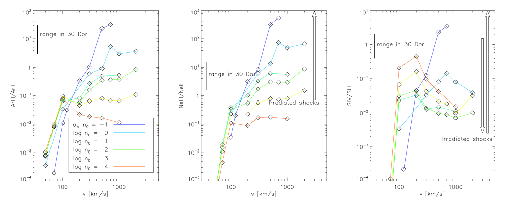
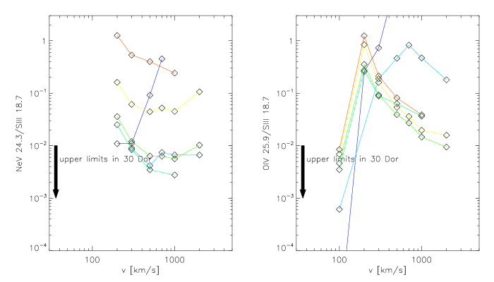
Figure 23: Ratios of line strengths calculated from plane-parallel shock models (the actual models that were run are diamonds, connected for clarity). Although the Ne, Ar, and S ratios can be produced by shocks of a few 100km s^-1 in diffuse gas, those shocks should also produce [O IV] emission, which we do not detect in 30 Doradus.

6 Conclusions

We present an infrared data cube of 30 Doradus, observed with the InfraRed Spectrograph and Multiband Imaging Spectrometer on the Spitzer Space Telescope. Aromatic dust emission features are of modest strength in the 30 Doradus region, concentrated in the arc-like two-lobed ridge coincident with CO emission and partially encircling the central R136 cluster. Detailed analysis of the dust content of the region from these features will follow in a subsequent publication, although the high average dust temperature is immediately obvious from the shape of the MIPS/SED spectrum. Of the pure rotational lines of molecular hydrogen, only S(3)$\lambda$9.67$\mu$m is detected with any significance, peaking on the bright “ridge” that dominates the morphology of the region at many wavelengths (see Fig 8). Low-ionization atomic lines are present but not particularly strong: [Si II] is detected in the outskirts of the mapped region, outside the region of strongest centimeter continuum (highest emission measure ionized gas). [Fe II] $\lambda$26.0$\mu$m is only tentatively detected in two locations.

Two hydrogen recombination lines Hu$\alpha$ (7-6) and Hu$\gamma$ (9-6) can be mapped over a large fraction of the observed area, and from these a relative measure of the extinction can be calculated. Independent estimates of the extinction are calculated from fitting the strength of the 10$\mu$m silicate feature, and from the ratio of H$\alpha$ to centimeter continuum. While none of the three extinction measures is extremely high signal-to-noise, the locations where all three show higher extinction should be quite secure - in particular three distinct locations in the west, southwest, and northeast, outside of the “ridge” (Fig 18).

The strongest atomic or molecular features in the data cube are the moderate-ionization ionic lines [Ar II]$\lambda$7.0$\mu$m, [Ar III]$\lambda$9.0$\mu$m, [Ne II]$\lambda$12.8$\mu$m, [Ne III]$\lambda$15.5$\mu$m, [S III]$\lambda$18.7$\mu$m, [S III]$\lambda$33.4$\mu$m, and [S IV]$\lambda$10.5$\mu$m. These lines are most sensitive to physical conditions in the ionized gas: the ionization parameter $U$ and hardness of the ionizing field, parametrized by the radiation temperature $T_{rad}$. We fit the Neon and Sulphur ratios with photoionization models to derive a 2-dimensional map of $U$ and $T_{rad}$. We find that the excitation generally follows the “ridge and bubble” morphology, and that under the assumptions of pure photoionization, there are “hot spots” of hardened ionizing field in the east of the bubble and between the two lobes of the ridge (corresponding to two molecular clouds). We also compare the line ratios to shock models and find poorer agreement with the data. In particular the nondetections of emission from more highly ionized species [O IV] and [Ne V] suggest that photoionization dominates over collisional excitation by shocks. Overall, the local effects of hot stars in 30 Doradus (such as the single WR star on the eastern side of the bubble) appear to dominate over any large-scale trend with distance from the central cluster R136.

Appendix A Flux calibration and adjustment

A.0.1 Background subtraction

Our off-target background observations bracket the data set in time. We chose to take an average (with minima and maxima trimmed) of all the background records and subtract that from all of the data records. It was possible that the two sets of background records could be appreciably different, reflecting a gradual change in the instrument (e.g. electronic drift), and that a linear interpolation of the two sets over time would be more appropriate as the background for each data record. Indeed, the mean flux level of our background records tends to increase with time, varying by 8% between the first and last exposures. Therefore, the average of the second set of background records has a higher mean flux level than the average of the first set.

We tested three different background subtractions on several apertures from the SL1 module: using only the first background set, using only the second, and using the mean of the two sets. The difference between the resulting spectra was very small. Specifically, the difference in continuum levels between typical spectra using the different background subtractions was on the order of 2%. For very low signal-to-noise spectra extracted from faint areas of the map, the continuum difference could reach 10%. We emphasize that, even then, the shape of the spectrum and the strength of the emission line features did not appreciably change. For the highest signal-to-noise spectra, the continuum difference was reduced to about 0.1%. We conclude that using the mean of all background records is adequate.

A.0.2 Flux calibration

The IRS SL slit is approximately 3.6 arcseconds wide, and the LL is approximately 10.6 arcseconds wide (see Spitzer Observer’s Manual 7.1, 2006, Table 7.5). Some fraction of the instrument point-spread function (PSF) falls outside of the slit, depending on wavelength. For example, the full width half max (FWHM) of the PSF at 14.5$\mu$m, at the upper wavelength range of the SL first order, is about 3.74 arcseconds (see Spitzer Observer’s Manual 7.1, 2006, §8.1.2.1). Optimized for point sources, the Spitzer Space Center pipeline adjusts the data for this loss of flux. However, in the case of a spatially uniform extended source, there is no net loss of flux. CUBISM can apply a slit loss correction factor which re-corrected the data to the original levels. In the case of 30 Doradus, an extended sources, we opted to do so. However, it is important to note that in some areas of the map, there are bright features which are neither point sources nor uniformly extended emission, which have some net loss of flux. The magnitude of this loss is at most 36% (see Sheth, 2006, Slide 13) . This loss may be responsible for some of the mismatches we experienced between the flux densities in the four different modules at some points in the map.

A.0.3 Final adjustments to the spectra

The wavelength range of the spectra needs to be trimmed. The full range of the IRS in each of the four modules includes bins where the response is unreliable. In the LL modules, where the spectrum of 30 Doradus is generally smooth, the drop in response at the long-wave edge of the LL2 module and the increase in noise at the long-wave edge of the LL1 module are evident.We trimmed the LL modules based on these observations. The spectrum of 30 Doradus is more complex in the SL modules, however, with many emission lines and an unclear continuum. In order to determine the range of wavelengths which can be trusted in each SL module, we examined the IRS low resolution staring mode spectrum of $\alpha$ Lacertae, an A1 dwarf star whose smooth spectrum is well known. In each of the SL modules, the spectrum departs from its smooth curve at the margins. We trimmed our SL spectra to the wavelengths where the IRS spectrum of $\alpha$ Lac stayed faithful to the smooth curve. We also found, based on some spectra from 30 Doradus, that the limit at the long-wave edge of the SL1 module based on the spectrum of $\alpha$ Lac was not conservative enough; consequently, we decreased the trusted upper limit on wavelength for the SL1. We could not use the spectrum of $\alpha$ Lac to determine the reliable wavelengths for the LL modules because the stellar spectrum has low signal-to-noise at such long wavelengths.

After extracting our spectra, we found that some of the SL spectra were suspiciously low, even negative for some counts. This may be a problem with background subtraction, and thus requires an additive correction. We raised both SL modules by the additive quantity necessary to make the floor of the SL2 spectrum (the median of the five lowest counts) non-negative. Over 72% of the map, this correction was unnecessary. Over the remaining 28%, mainly in areas of low signal, the SL spectrum was raised by a mean level of 5.5 MJy/sr, with standard deviation of 6.5 MJy/sr. For comparison, the mean level of the background spectrum in the SL is 3.2 MJy/sr and the mean level of the background-subtracted SL spectrum averaged across a large region of 30 Doradus is about 100 MJy/sr.

The different modules of an IRS spectrum do not always match up well in flux density. The mismatches between the SL1 and SL2 modules, and between the LL1 and LL2 modules, were rarely serious. However, we noticed more consistent mismatches between the SL1 and LL2 modules. The primary cause is probably that the emission in the 30 Doradus region is often best characterized as neither a point source nor as a uniform extended source, but instead as something in between. We have treated it as a uniform extended source (see §A.0.2), likely losing some flux. This would call for a multiplicative correction. We found logarithmic fits to the continuum emission close to the junction in each module and multiplied the SL spectra by the ratio of the fits in the overlapping wavelengths. The mean value of the multiplicative correction is 1.2 with a standard deviation of 1.2.

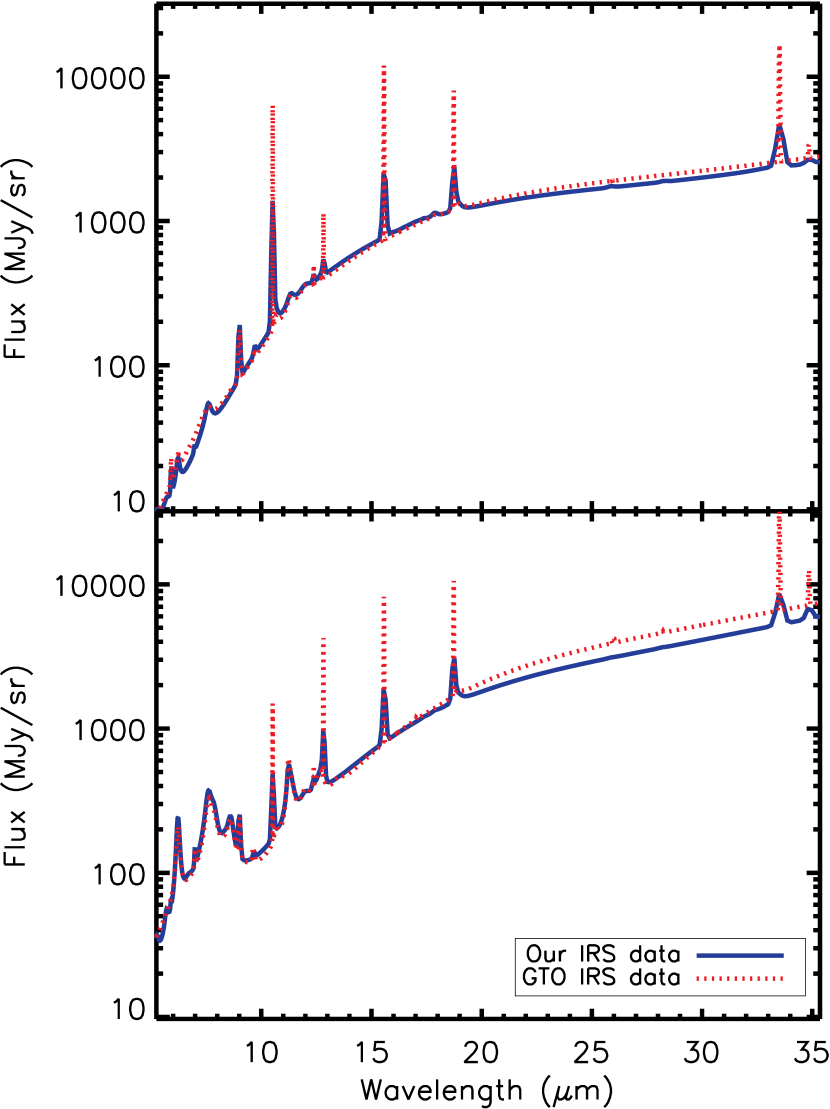
Figure 24: In blue, the fit to our low resolution spectra. In red, the same type of fit applied to the high resolution GTO spectra, with high resolution data at long wavelengths combined with low resolution data at short wavelengths (the transition is at about 10$\mu$m). Top: a relatively faint area in the southern part of the 30 Doradus nebula. Bottom: a brighter area, where the low resolution spectrum suffers from partial saturation and falling response in the LL1 module.

Figure 25: Two comparisons of our low-resolution IRS data to high-resolution IRS data from Lebouteiller et al. (2007). (The two panels are drawn from different regions on the sky, but for each panel the high and low resolution spectra are both extracted from the same aperture on the sky.) Both the measured spectra (symbols) and our fits made with PAHFIT (solid and dotted lines) are displayed. Note that while the high resolution spectrum has higher resolution for the lines, and the continuum strength may vary, the overall strength of the lines agree. Also note that the PAH has a fairly smooth appearance in the low-resolution plot and a more complex morphology in the high-resolution spectrum, which can cause problems when attempting to fit PAH strength in high-resolution. See Appendix B.

Figure 26: Comparison of the fitted integrated strengths of four emission lines. On the horizontal axis are the results from our low resolution spectra. On the vertical axis are the results of using the same type of fit on the GTO spectra, which are high resolution longward of about 10 $\mu$m. Each symbol represents one area of the 30 Doradus nebula, with horizontal and vertical error bars. The discrepancies from the line of unity are discussed in Appendix B. Among those discrepancies, the fitting algorithm we used is not designed to fit the more complex structure of PAHs that is resolved in the high resolution spectrum. Another reason for the discrepancy in the Humphreys-$\alpha$ is that our fits to the line also include the fainter H₂ S(2) $\lambda$12.28$\mu$m emission line, which is not well resolved at low resolution. The square symbols in the lower right plot call attention to two outlying points discussed in Appendix  B.

Appendix B Quality Assurance

In order to check our work on reducing the spectral map, we compared our spectra, taken with the low resolution modules of the IRS in mapping mode, to spectra of several areas of the 30 Doradus nebula taken with both the low and high resolution modules of the IRS, in staring mode (private correspondence and Lebouteiller et al., 2007). These spectra will henceforth be referred to as the GTO spectra. The apertures they span are displayed in green in Figure 3. By selecting the subsets of our map that coincide with the GTO apertures, we can produce spectra which should be consistent with theirs. We applied PAHFIT, the same fitting algorithm that we use on our spectral map, to the GTO spectra. We made some adjustments to PAHFIT to allow for the much higher spectral resolution in the GTO spectra redward of about 10$\mu$m, where there is coverage from the high resolution modules.

In Figure 24, the fitted spectra from two of these apertures are shown. The overall agreement in the shape of the spectrum is clear, with a notable exception in the continuum from 20 to 32$\mu$m(likely the result of nonlinearity in the short-low detector response). In the upper panel, taken from an aperture toward the south of the 30 Doradus nebula, at around 05^h38^m50^s -69^∘06′41″, where the continuum emission at long wavelengths is relatively faint, the agreement between the GTO spectrum and ours is close, but the effect starts to become noticeable at higher flux densities. In the lower panel, taken from a brighter part of the 30 Doradus nebula at 05^h38^m48^s -69^∘04′10″ where the falling response in the LL1 is more severe, the difference between the GTO spectrum and ours is larger.

We are most concerned with whether we can obtain the same emission line strengths by fitting the GTO spectra in the same manner as ours. Figures 24 and 25 show that the PAHs have similar profiles, while the unresolved atomic lines are narrower with higher central intensities in the long-wave, high resolution part of the GTO spectra. The integrated strengths of several of the long-wave emission lines of interest are plotted in Figure 26, for twelve GTO spectra and the corresponding apertures in our map. Perfect agreement falls along the line of unity.

The fits to the PAH complex at 11.3$\mu$m agree well only at low strength. This may be because of detailed fine structure that appears in the PAH complex at high resolution. In the low resolution spectrum, only a broad feature at 11.3$\mu$m, with a shoulder at 11.0$\mu$m, is apparent. A Drude profile is sufficient to fit that, and a more complex fitting profile would not be appropriate because of the lack of resolution. In high resolution such as in the GTO spectra, the shoulder at 11.0$\mu$m resolves into a completely separate feature (see Figure 25), possibly another PAH feature. This might also be the Paschen-$\gamma$ HI recombination line, although so significantly shifted from its rest wavelength at 10.95$\mu$m as to make such an identification questionable. The main PAH feature at 11.3$\mu$m displays a different profile that would require a more complex fitting algorithm. Thus, we are not concerned about this disparity. The conclusion is that PAHFIT is adequate for fitting PAHs at low resolution, but may not sufficiently describe the same features at high resolution – not surprising, as the list of features used in PAHFIT was empirically tuned using low resolution spectra.

A systematic disparity is evident in the comparison of the Humphreys-$\alpha$ $\lambda$12.37$\mu$m fitted line strength. Upon closer examination, two factors surfaced. Both support the trend that the fitted line strength at low resolution is higher than the line strength at high resolution. First, the fainter molecular hydrogen line, H₂ S(2) $\lambda$12.28$\mu$m, is resolved in high resolution. The fit to the high resolution Humphreys-$\alpha$ line therefore does not include any of the flux from the molecular hydrogen line. Meanwhile, in the low resolution spectrum, the flux from both lines contributes to the same broad feature. We are confident that Humphreys-$\alpha$ contributes most of the flux we see in low resolution, in part because the line center more closely coincides with 12.37 than with 12.28$\mu$m, and in part because, as we can see in the high resolution spectra, the Humphreys-$\alpha$ line is equal to or stronger than H₂ S(2) in all of the areas of our map covered by the high resolution spectra. However, the flux of both emission lines is contributing to the low-resolution fit, and so to some extent, our fits to the line strength of the Humphreys-$\alpha$ line are overestimated. Quantitative comparison between high- and low-resolution spectra and between fits with and without the molecular hydrogen line show that the contamination of the Humphreys-$\alpha$ line strength is at most $\sim$20% (see §4.1). This effect is weakest in the parts of 30 Doradus dominated by ionized gas that are the focus of this paper, but should be kept in mind for analysis of the outer parts of the region and PDR physics in future papers. The second factor that contributes to the disparity seen in the second panel of Figure 26 is the PAH feature at 12.6$\mu$m. As discussed above in the context of the PAH complex at 11.3$\mu$m, the fitting package PAHFIT is intended for the relatively smooth features seen in low resolution, and does not handle the complex morphology of PAHs seen at high resolution as well. In the case of the PAH at 12.6$\mu$m, its line strength in the high resolution fit is generally overestimated. Its broad wings thus lead the strength of the Humphreys-$\alpha$ line to be underestimated in the high resolution fit. The slight overestimation of the line in the low resolution spectrum and the slight underestimation of the line in the high resolution spectrum both contribute to the disparity.

The results for the forbidden neon lines, as for most of the stronger lines, show a tighter correlation. The close agreement in the fits to the low and high resolution spectra for the weaker [Ne II]$\lambda$12.8$\mu$m is particularly encouraging because one of our concerns in interpreting the neon ratio was the possible entanglement of the [Ne II] atomic emission line with the above-mentioned PAH at 12.6$\mu$m. In the high resolution spectrum, the PAH (with its often-unusual shape) and the atomic line are resolved. As in the case of the Humphreys-$\alpha$ line, the strength of the [Ne II] line may be slightly underestimated because of the poor, overestimated fit to the PAH at 12.6$\mu$m. The close agreement between the low resolution and high resolution fit, across almost all of the twelve apertures, regardless of PAH strength in each aperture, indicates that there are no systematic errors to the low resolution fit that do not also appear in the high resolution fit. Thus, our results may share the slight bias toward underestimating the [Ne II] strength, but we are generally able to decompose [Ne II] and the PAH at 12.6$\mu$m despite the lack of spectral resolution.

Finally, the correlation for the fitted line strength of [Ne III]$\lambda$15.5$\mu$m is similarly good, with the exception of two apertures where the high resolution fitted line strength is significantly higher than the low resolution fitted line strength. These two apertures (displayed with squares rather than diamonds in Figure 26) are located in a small region of the map that exemplifies the extreme of the trend shown in Figure 24, where the response in the LL1 module falls until the module finally saturates. In these cases, our fit to the continuum with thermal dust components is not very successful. The fitted continuum is dragged down in the area from 20 to 32$\mu$m, which forces it up in the region of 15$\mu$m. This causes our estimation of the strength of [Ne III] to be underestimated.

For these two anomalous apertures, we conducted a test by removing the faulty LL1 spectrum and fitting only the remaining spectrum, to get a better estimation of continuum in the region of [Ne III]. This increased the fitted strength of [Ne III], though not enough to get it to agree with the value we obtained by fitting the high-resolution spectrum.

The effect of long-wave line strengths being underestimated in our low resolution spectra compared to the high resolution GTO spectra is seen for [Ne III]$\lambda$15.5$\mu$m and [S III]$\lambda$33.4$\mu$m in some areas of the map. Empirically, the line strengths of [Ne II]$\lambda$12.8$\mu$m and [S III]$\lambda$18.7$\mu$m appear to be unaffected, as shown by their close agreement with the GTO spectra. It is crucial to note that this effect is restricted to the small areas of the map where we can see falling response in the LL1 module, as drawn in Figure 4. In that localized area, we can expect our values of [Ne III] and [S III]$\lambda$33.4$\mu$m to be underestimated relative to the GTO results by perhaps 30%, as shown in Figure 26 (the effect is very similar for [S III]$\lambda$33.4$\mu$m). Outside these small areas of the map, the agreement between our spectra and the high-resolution GTO spectra is excellent for these two emission lines.

ACKNOWLEDGMENTS

This work benefited greatly from the generous contributions of several individuals: Gary Ferland and his students for creating the Cloudy photoionization code, John Raymond for giving us a copy of his shock code, John Dickel and Jasmina Lazendic for giving us their calibrated centimeter synthesis images, and Sean Points for giving us calibrated MCELS H$\alpha$ data. This publication would not have been possible without extensive use of NASA’s Astrophysics Data System Bibliographic Services, and the SIMBAD database, operated at CDS, Strasbourg, France. This publication makes use of data products from the Two Micron All Sky Survey, which is a joint project of the University of Massachusetts and the Infrared Processing and Analysis Center/California Institute of Technology, funded by NASA and NSF. Data from the Spitzer Space Telescope (operated by the Jet Propulsion Lab for NASA) are taken from PID 30653 “Stellar Feedback on Circumcluster Gas and Dust in 30 Doradus, the Nearest Super-Star Cluster” and PID 20203 “Spitzer Survey of the Large Magellanic Cloud: Surveying the Agents of a Galaxy’s Evolution (SAGE)” GdM and RI were supported in part by Spitzer/NASA/JPL grant #1288328, and RI in part by a Spitzer fellowship to UVa. Meixner and Sewilo were supported in part by Spitzer/NASA/JPL grants #1288277 and #1275598.

Facilities: Spitzer (IRS)

References

- Abel & Satyapal (2008) Abel, N. P., & Satyapal, S. 2008, ArXiv e-prints, 801, arXiv:0801.2766
- Asplund et al. (2005) Asplund, M., Grevesse, N., & Sauval, A. J. 2005, Cosmic Abundances as Records of Stellar Evolution and Nucleosynthesis, 336, 25
- Bernard et al (2008) Bernard, J.P. 2008, AJ submitted.
- Brandner et al. (2001) Brandner, W., Grebel, E. K., Barbá, R. H., Walborn, N. R., & Moneti, A. 2001, AJ, 122, 858
- Breysacher et al. (1999) Breysacher, J., Azzopardi, M., & Testor, G. 1999, A&AS, 137, 117
- Castelli & Kurucz (2004) Castelli, F., & Kurucz, R. L. 2004, ArXiv Astrophysics e-prints, arXiv:astro-ph/0405087
- Chiar & Tielens (2006) Chiar, J. E., & Tielens, A. G. G. M. 2006, ApJ, 637, 774
- Chu et al. (2004) Chu, Y.-H., Gruendl, R. A., Chen, C.-H. R., Lazendic, J. S., & Dickel, J. R. 2004, ApJ, 615, 727
- Cox & Raymond (1985) Cox, D. P., & Raymond, J. C. 1985, ApJ, 298, 651
- Dickel et al. (1994) Dickel, J. R., Milne, D. K., Kennicutt, R. C., Chu, Y.-H., & Schommer, R. A. 1994, AJ, 107, 1067
- Dopita et al. (2006) Dopita, M. A., et al. 2006, ApJ, 639, 788
- Dudik et al. (2007) Dudik, R. P., Weingartner, J. C., Satyapal, S., Fischer, J., Dudley, C. C., & O’Halloran, B. 2007, ApJ, 664, 71
- Fazio et al. (2004) Fazio, G. G., et al. 2004, ApJS, 154, 10
- Ferland et al. (1998) Ferland, G. J., Korista, K. T., Verner, D. A., Ferguson, J. W., Kingdon, J. B., & Verner, E. M. 1998, PASP, 110, 761
- France et al. (2007) France, K., McCandliss, S. R., & Lupu, R. E. 2007, ApJ, 655, 920
- Galliano et al. (2008) Galliano, F., Dwek, E., & Chanial, P. 2008, ApJ, 672, 214
- Gordon et al. (2007) Gordon, K. D., et al. 2007, PASP, 119, 1019
- Hartigan et al. (1987) Hartigan, P., Raymond, J., & Hartmann, L. 1987, ApJ, 316, 323
- Hollenbach & McKee (1989) Hollenbach, D., & McKee, C. F. 1989, ApJ, 342, 306
- Houck et al. (2004) Houck, J. R., et al. 2004, Proc. SPIE, 5487, 62
- Hubeny & Lanz (1995) Hubeny, I., & Lanz, T. 1995, ApJ, 439, 875
- Hunter (1999) Hunter, D.A. 1999, IAUS, 190, 217
- Hyland et al. (1992) Hyland, A. R., Straw, S., Jones, T. J., & Gatley, I. 1992, MNRAS, 257, 391
- Indebetouw et al. (2005) Indebetouw, R., et al. 2005, ApJ, 619, 931
- Johansson et al. (1998) Johansson, L. E. B., et al. 1998, A&A, 331, 857
- Johnson (2004) Johnson, K. E. 2004, New A Rev., 48, 1337
- Kim (2007) Kim, S. 2007, The Seventh Pacific Rim Conference on Stellar Astrophysics, 362, 297
- Lacy et al. (2007) Lacy, J. H., et al. 2007, ApJ, 658, L45
- Lazendic et al. (2003) Lazendic, J. S., Dickel, J. R., & Jones, P. A. 2003, ApJ, 596, 287
- Lebouteiller et al. (2007) Lebouteiller, V., Bernard-Salas, J., Brandl, B., Whelan, D., Wu, Y., Charmandaris, V., & Devost, D. 2007, ArXiv e-prints, 710, arXiv:0710.4549
- Lefloch et al. (2003) Lefloch, B., Cernicharo, J., Cabrit, S., Noriega-Crespo, A., Moro-Martín, A., & Cesarsky, D. 2003, ApJ, 590, L41
- Lodders (2003) Lodders, K. 2003, ApJ, 591, 1220
- Lodders (2007) Lodders, K. 2007, ArXiv e-prints, 710, arXiv:0710.4523
- Lu et al. (2008) Lu, N., et al. 2008, ArXiv e-prints, 802, arXiv:0802.3723
- Maercker & Burton (2005) Maercker, M., & Burton, M. G. 2005, A&A, 438, 663
- Madden et al. (2006) Madden, S. C., Galliano, F., Jones, A. P., & Sauvage, M. 2006, A&A, 446, 877
- Martín-Hernández et al. (2002) Martín-Hernández, N. L., et al. 2002, A&A, 381, 606
- Meixner et al. (2006) Meixner, M., et al. 2006, AJ, 132, 2268
- Mendoza & Zeippen (1982) Mendoza, C., & Zeippen, C. J. 1982, MNRAS, 199, 1025
- Morisset et al. (2004) Morisset, C., Schaerer, D., Bouret, J.-C., & Martins, F. 2004, A&A, 415, 577
- Molinari & Noriega-Crespo (2002) Molinari, S., & Noriega-Crespo, A. 2002, AJ, 123, 2010
- Neufeld et al. (2006) Neufeld, D. A., et al. 2006, ApJ, 649, 816
- Neufeld et al. (2007) Neufeld, D. A., Hollenbach, D. J., Kaufman, M. J., Snell, R. L., Melnick, G. J., Bergin, E. A., & Sonnentrucker, P. 2007, ApJ, 664, 890
- Noriega-Crespo et al. (2004) Noriega-Crespo, A., et al. 2004, ApJS, 154, 352
- Noriega-Crespo et al. (2004) Noriega-Crespo, A., Moro-Martin, A., Carey, S., Morris, P. W., Padgett, D. L., Latter, W. B., & Muzerolle, J. 2004, ApJS, 154, 402
- Okamoto et al. (2001) Okamoto, Y. K., Kataza, H., Yamashita, T., Miyata, T., & Onaka, T. 2001, ApJ, 553, 254
- Parker (1993) Parker, J. W. 1993, AJ, 106, 560
- Peck et al. (1997) Peck, A. B., Goss, W. M., Dickel, H. R., Roelfsema, P. R., Kesteven, M. J., Dickel, J. R., Milne, D. K., & Points, S. D. 1997, ApJ, 486, 329
- Peeters et al. (2002) Peeters, E., et al. 2002, A&A, 381, 571
- Poglitsch et al. (1995) Poglitsch, A., Krabbe, A., Madden, S. C., Nikola, T., Geis, N., Johansson, L. E. B., Stacey, G. J., & Sternberg, A. 1995, ApJ, 454, 293
- Rakowski et al. (2007) Rakowski, C. E., Raymond, J. C., & Szentgyorgyi, A. H. 2007, ApJ, 655, 885
- Raymond (1979) Raymond, J. C. 1979, ApJS, 39, 1
- Rieke et al. (2004) Rieke, G. H., et al. 2004, ApJS, 154, 25
- Rubio et al. (1998) Rubio, M., Barbá, R. H., Walborn, N. R., Probst, R. G., García, J., & Roth, M. R. 1998, AJ, 116, 1708
- Rosa & Mathis (1987) Rosa, M., & Mathis, J. S. 1987, ApJ, 317, 163
- Shaver et al. (1983) Shaver, P. A., McGee, R. X., Newton, L. M., Danks, A. C., & Pottasch, S. R. 1983, MNRAS, 204, 53
- Schaefer (2008) Schaefer, B. E. 2008, AJ, 135, 112
- Schaerer & de Koter (1997) Schaerer, D., & de Koter, A. 1997, A&A, 322, 598
- Sheth (2006) Sheth, K. 2006, in Spitzer Data Analysis Workshop #4.
- Simpson et al. (2007) Simpson, J. P., Colgan, S. W. J., Cotera, A. S., Erickson, E. F., Hollenbach, D. J., Kaufman, M. J., & Rubin, R. H. 2007, ArXiv e-prints, 708, arXiv:0708.2103
- Smith (2007a) Smith, J.D.T., et al. 2007, ApJ, 656, 770
- Smith (2007b) Smith, J.D.T., et al. 2007, PASP, 119, 1133
- Smith et al. (2002) Smith, L. J., Norris, R. P. F., & Crowther, P. A. 2002, MNRAS, 337, 1309
- Sofia & Jenkins (1998) Sofia, U. J., & Jenkins, E. B. 1998, ApJ, 499, 951
- Spitzer Observer’s Manual 7.1 (2006) Spitzer Science Center. 2006, Spitzer Space Telescope Observer’s Manual, Version 7.1, Spitzer Science Center
- Stasińska & Schaerer (1997) Stasińska, G., & Schaerer, D. 1997, A&A, 322, 615
- Sturm et al. (2000) Sturm, E., Lutz, D., Tran, D., Feuchtgruber, H., Genzel, R., Kunze, D., Moorwood, A. F. M., & Thornley, M. D. 2000, A&A, 358, 481
- Tayal & Gupta (1999) Tayal, S. S., & Gupta, G. P. 1999, ApJ, 526, 544
- Townsley et al. (2006) Townsley, L. K., Broos, P. S., Feigelson, E. D., Brandl, B. R., Chu, Y.-H., Garmire, G. P., & Pavlov, G. G. 2006, AJ, 131, 2140
- Tsamis & Péquignot (2005) Tsamis, Y. G., & Péquignot, D. 2005, MNRAS, 364, 687
- Vermeij et al. (2002) Vermeij, R., Peeters, E., Tielens, A. G. G. M., & van der Hulst, J. M. 2002, A&A, 382, 1042
- Walborn (1991) Walborn, N.R. 1991, IAUS, 148, 145
- Weingartner & Draine (2001) Weingartner, J. C., & Draine, B. T. 2001, ApJ, 548, 296.
- Werner et al. (2004) Werner, M. W., et al. 2004, ApJS, 154, 1