Invertible Extractors and Wiretap Protocols

Abstract

A wiretap protocol is a pair of randomized encoding and decoding functions such that knowledge of a bounded fraction of the encoding of a message reveals essentially no information about the message, while knowledge of the entire encoding reveals the message using the decoder. In this paper we study the notion of efficiently invertible extractors and show that a wiretap protocol can be constructed from such an extractor. We will then construct invertible extractors for symbol-fixing, affine, and general sources and apply them to create wiretap protocols with asymptotically optimal trade-offs between their rate (ratio of the length of the message versus its encoding) and resilience (ratio of the observed positions of the encoding and the length of the encoding). We will then apply our results to create wiretap protocols for challenging communication problems, such as active intruders who change portions of the encoding, network coding, and intruders observing arbitrary boolean functions of the encoding.
As a by-product of our constructions we obtain new explicit extractors for a restricted family of affine sources over large fields (that in particular generalizes the notion of symbol-fixing sources) which is of independent interest. These extractors are able to extract the entire source entropy with zero error.

Keywords: Wiretap Channel, Extractors, Network Coding, Active Intrusion, Exposure Resilient Cryptography.

I Introduction

Suppose that Alice wants to send a message to Bob through a communication channel, and that the message is partially observable by an intruder. This scenario arises in various practical situations. For instance, in a packet network, the sequence transmitted by Alice through the channel can be fragmented into small packets at the source and/or along the way. Then, different packets might be routed through different paths in the network in which an intruder may have compromised some of the intermediate routers. An example that is similar in spirit is furnished by transmission of a piece of information from multiple senders to one receiver, across different delivery media, such as satellite, wireless, and/or wired networks. Due to limited resources, a potential intruder may be able to observe only a fraction of the lines of transmission, and hence only partially observe the message. As another example, one can consider secure storage of data on a distributed medium that is physically accessible in parts by an intruder, or a sensitive file on a hard drive that is erased from the file system but is only partially overwritten with new or random information, and hence, is partially exposed to a malicious party.

An obvious approach to solve this problem is to use a secret key to encrypt the information at the source. However, almost all practical cryptographic techniques are shown to be secure only under unproven hardness assumptions and the assumption that the intruder possesses bounded computational power. This might be undesirable in certain situations. Moreover, the key agreement problem has its own challenges.

In this paper, we assume the intruder to be information theoretically limited, and our goal will be to employ this limitation and construct a protocol that provides unconditional, information-theoretic security, even in the presence of a computationally unbounded adversary.

The problem described above was first formalized by Wyner [1] and subsequently by Ozarow and Wyner [2] as an information-theoretic problem. In its most basic setting, this problem is known as the wiretap II problem (the description given here follows from [2]):

Consider a communication system with a source which outputs a sequence $X=(X_{1},\ldots,X_{m})$ in $\{0,1\}^{m}$ uniformly at random. A randomized algorithm, called the encoder, maps the output of the source to a binary string $Y\in\{0,1\}^{n}$. The output of the encoder is then sent through a noiseless channel (called the direct channel) and is eventually delivered to a decoder $D$ which maps $Y$ back to $X$. Along the way, an intruder arbitrarily picks a subset $S\subseteq[n]:=\{1,\ldots,n\}$ of size $t\leq n$, and is allowed to observe $W:=Y|_{S}$ (through a so-called wiretap channel), i.e., $Y$ on the coordinate positions corresponding to the set $S$. The goal is to make sure that the intruder learns as little as possible about $X$, regardless of the choice of $S$.

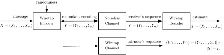
Figure 1: The Wiretap II Problem.

The system defined above is illustrated in Fig. 1. The security of the system is defined by the following conditional entropy, known as “equivocation”:

$$\Delta:=\min_{S\colon|S|=t}H(X|W).$$

When $\Delta=H(X)=m$, the intruder obtains no information about the transmitted message and we have perfect privacy in the system. Moreover, when $\Delta\to m$ as $m\to\infty$, we call the system asymptotically perfectly private. These two cases correspond to what is known in the literature as “strong secrecy”. A weaker requirement (known as “weak secrecy”) would be to have $m-\Delta=o(m)$.

Remark 1.

The assumption that $X$ is sampled from a uniformly random source should not be confused with the fact that Alice is transmitting one particular message to Bob that is fixed and known to her before the transmission. In this case, the randomness of $X$ in the model captures the a priori uncertainty about $X$ for the outside world, and in particular the intruder, but not the transmitter.

As an intuitive example, suppose that a random key is agreed upon between Alice and a trusted third party, and now Alice wishes to securely send her particular key to Bob over a wiretapped channel. Or, assume that Alice wishes to send an audio stream to Bob that is encoded and compressed using a conventional audio encoding method.

Furthermore, the particular choice of the distribution on $X$ as a uniformly random sequence will cause no loss of generality. If the distribution of $X$ is publicly known to be non-uniform, the transmitter can use a suitable source-coding scheme to compress the source to its entropy prior to the transmission, and ensure that from the intruder’s point of view, $X$ is uniformly distributed. On the other hand, it is also easy to see that if a protocol achieves perfect privacy under uniform message distribution, it achieves perfect privacy under any other distribution as well.

The main focus of this paper is on asymptotic trade-offs between the rate $R:=m/n$ and the resilience $\delta:=t/n$ of an asymptotically perfectly private wiretap coding scheme. We will focus on the case where the fraction $\delta$ of the symbols observed by the intruder is an arbitrary constant below $1$, which is the most interesting range in our context. However, some of our constructions work for sub-constant $1-\delta$ as well.

Following [2], it is easy to see that, for resilience $\delta$, an information-theoretic bound $R\leq 1-\delta+o(1)$ must hold. Lower bounds for $R$ in terms of $\delta$ have been studied by a number of researchers.

For the case of perfect privacy (where the equivocation $\Delta$ is exactly equal to the message length), Ozarow and Wyner [2] give a wiretap coding scheme using linear error-correcting codes, and show that the existence of an $[n,k,d]_{q}$-code implies the existence of a perfectly private wiretap coding scheme with message length $k$ and block length $n$ (thus, rate $k/n$) and resilience $\delta=(d-1)/n$.

As a result, the so-called Gilbert-Varshamov bound on the rate-distance trade-offs of linear codes [3, 4] implies that, asymptotically, $R\geq 1-h_{q}(\delta)$, where $h_{q}$ is the $q$-ary entropy function defined as

$$h_{q}(x):=x\log_{q}(q-1)-x\log_{q}(x)-(1-x)\log_{q}(1-x).$$

If $q\geq 49$ is a square, the bound can be further improved to $R\geq 1-\delta-1/(\sqrt{q}-1)$ using Goppa’s algebraic-geometric codes [5, 6].

Moving away from perfect to asymptotically perfect privacy, it was (implicitly) shown in [7] that for any $\gamma>0$ there exist binary asymptotically perfectly private wiretap coding schemes with $R\geq 1-2\delta-\gamma$ and exponentially small error. This bound strictly improves the coding-theoretic bound of Ozarow and Wyner for the binary alphabet.

I-A Overview of our Results

In this paper we prove several lower bounds for the rate of asymptotically perfectly private wiretap protocols with negligible, i.e., superpolynomially small, error. This is shown constructively; i.e., by demonstrating polynomial-time computable encoding and decoding schemes that achieve the lower bounds. Our main tool is the design of various types of invertible extractors, a concept defined in Section V.

The formal model that our results are based on is defined in Section III. As we will see, this model is more stringent than the original Wiretap II problem. In Section IV, we review a known construction of symbol-fixing extractors based on linear codes. Then we extend this result to the case of “restricted” affine sources, using rank-metric codes. Using these extractors, we are able to recover Ozarow and Wyner’s coding-based wiretap schemes as well as a recent construction of wiretap schemes for network coding (due to Silva and Kschischang [8], discussed in Section VIII-B) in our framework.

Our next construction, described in Section VI, shows that if the alphabet size is $d$, then there exists $\alpha_{d}\in(0,1)$ such that for every $\eta>0$ and every constant resilience $\delta\in[0,1)$, we essentially have rate $R\geq\max\{\alpha_{d}(1-\delta),1-\delta/\alpha_{d}\}-\eta$ with exponentially small error. This is achieved by suitably modifying the symbol-fixing extractor of Kamp and Zuckerman [9]. Contrary to the coding theoretic construction of Ozarow and Wyner, for a fixed alphabet size our bound gives a positive rate for every constant resilience $\delta\in[0,1)$.

Even though the bound in Section VI is superceded by our main result in Section VII, we have included it because of its simplicity and potential for practical use. Our second bound (Theorem 29) matches the information-theoretic upper bound of Ozarow and Wyner. Namely, for any prime power alphabet size $q$, and any resilience $\delta\in[0,1)$, we construct a wiretap protocol with superpolynomially small error, zero leakage and rate $\geq 1-\delta-o(1)$. In fact, this bound holds in a more general setting in which the intruder is not only allowed to look at a $\delta$-fraction of the symbols of Alice’s message, but is also allowed to perform any linear preprocessing of Alice’s message before doing so. The power of this result stems largely from a black box transformation which makes certain seedless extractors invertible. More specifically, the results of this section are obtained by applying this transformation to certain affine extractors. A plot of the bounds (which also compares our bounds with those obtained in other relevant works) can be found in Fig. 2.

Figure 2: A comparison of the rate vs. resilience trade-offs achieved by the wiretap protocols for the binary alphabet (left) and larger alphabets (right, in this example of size $64$). $(1)$ Information-theoretic bound, attained by Theorem 29; $(2)$ The bound approached by [7]; $(3)$ Protocol based on best non-explicit binary linear codes [3, 4]; $(4)$ The construction of [10] (based on all-or-nothing transforms), assuming that the underlying exposure-resilient function is optimal (see Appendix -D for a discussion); $(5)$ Random walk protocol of Corollary 23, using a Ramanujan graph; $(6)$ Protocol based on the best known explicit [6] and non-explicit [3, 4] linear codes.

In sections VIII-A and VIII-B, we will demonstrate several important applications of this fact in the context of network coding as well as wiretapped communication in the presence of noise and active intruders. In particular we provide, for the first time, an optimal solution to the wiretap problem in network coding [11] without imposing any restrictions (such as a large alphabet or packet length, or any change in the network code). We remark that our coding scheme adds a privacy layer to any existing network coding scheme as an outer code, without affecting the existing code being used. Thus, the resulting network coding scheme may be made resilient against noise (or active intruders) if the original network code can handle errors.

The final application in Section VIII-C studies an all-powerful intruder who is only limited by the amount of information he can obtain from Alice’s encoded message, and not by the nature of the observations. By inverting seeded extractors with nearly-optimal output lengths, we will show that if Alice and Bob have access to a side channel over which Alice can publicly send a polylogarithmic number of bits to Bob (that can be seen by the eavesdropper), then their communication on the main channel can be made secure even if the intruder can access the values of any $t$ Boolean functions of Alice’s encoded message.

II Preliminaries and Basic Facts

II-A Notation and Probability Distributions

For a prime power $q$, we use $\mathds{F}_{q}$ to denote the finite field with $q$ elements. We will occasionally use the notation $\mathds{F}_{2}$ for the set $\{0,1\}$, even if we do not need to use the field structure. For a positive integer $n$, define $[n]$ as the set $\{1,2,\ldots,n\}$. For a vector $x=(x_{1},x_{2},\ldots,x_{n})$ and a subset $S\subseteq[n]$, we denote by $x|_{S}$ the vector of length $|S|$ that is obtained from $x$ by removing all the coordinates $x_{i}$, $i\notin S$. For an integer $k>0$, we will use the notation $\mathcal{U}_{k}$ for the uniform distribution on $\mathds{F}_{2}^{k}$. More generally, for a finite set $\Omega$, we will use $\mathcal{U}_{\Omega}$ for the uniform distribution on $\Omega$. For a function $f$, we denote by $f^{-1}(x)$ the set of the preimages of $x$, i.e., the set $\{y\colon f(y)=x\}$. We denote the probability measure defined by a distribution $\mathcal{X}$ by $\Pr_{\mathcal{X}}$, hence, $\Pr_{\mathcal{X}}(x)$ and $\Pr_{\mathcal{X}}[S]$ for $x\in\Omega$ and $S\subseteq\Omega$ denote the probability that $\mathcal{X}$ assigns to an outcome $x$ and an event $S$, respectively. We will use $\mathcal{X}|S$ to denote the conditional distribution of $\mathcal{X}$ restricted to the set (event) $S$, and $X\sim\mathcal{X}$ to denote that a random variable $X$ is distributed according to $\mathcal{X}$.

Definition 2.

The support of a distribution is the set of all the elements of the sample space to which it assigns nonzero probabilities. The min-entropy of a distribution $\mathcal{X}$ with finite support $S$ is defined as

$$H_{\infty}(\mathcal{X}):=\min_{x\in S}\{-\log\Pr_{\mathcal{X}}(x)\},$$

where typically $\log(\cdot)$ is the logarithm function in base $2$. However, when $\mathcal{X}$ is supported on a set of $d$-ary strings, we find it more convenient to use the logarithm function in base $d$ and measure the entropy in $d$-ary symbols instead of bits. The Shannon entropy of the distribution, on the other hand, is defined as

$$H(\mathcal{X}):=\sum_{x\in S}(-\Pr_{\mathcal{X}}(x)\log\Pr_{\mathcal{X}}(x)).$$

When a distribution defined on the set of $n$-bit strings has min-entropy $k$, the quantity $k/n$ defines the entropy rate of the distribution. Note that the above definition immediately implies that the min-entropy of a distribution is upper bounded by its Shannon entropy (which is in fact the “expectation” of the logarithm of the probabilities). Hence, if the min-entropy of a distribution is at least $h$, its Shannon-entropy is also at least $h$. These two measures however coincide for uniform distributions.

Definition 3.

The statistical distance (or total variation distance) of two distributions $\mathcal{X}$ and $\mathcal{Y}$ defined on the same finite space $S$ is given by

$$\frac{1}{2}\sum_{s\in S}|\Pr_{\mathcal{X}}(s)-\Pr_{\mathcal{Y}}(s)|,$$

and is denoted by ${\mathsf{dist}}(\mathcal{X},\mathcal{Y})$. Note that this is half the $\ell_{1}$ distance of the two distributions when regarded as vectors of probabilities over $S$.

It can be shown that the statistical distance of the two distributions is at most $\epsilon$ if and only if for every $T\subseteq S$, we have $|\Pr_{\mathcal{X}}[T]-\Pr_{\mathcal{Y}}[T]|\leq\epsilon$. When the statistical distance of $\mathcal{X}$ and $\mathcal{Y}$ is at most $\epsilon$, they are said to be $\epsilon$-close and this is denoted by $\mathcal{X}\sim_{\epsilon}\mathcal{Y}$.

While we defined the above terms for probability distributions, with a slight abuse of notation we may use them interchangeably for random variables as well.

III The Formal Model

The model that we consider in this work is motivated by the original wiretap channel problem but is more stringent in terms of its security requirements. In particular, instead of using Shannon entropy as a measure of uncertainty, we will rely on statistical indistinguishability which is a stronger measure that is more widely used in cryptography.

Definition 4.

Let $\Sigma$ be a set of size $d$, parameters $m$ and $n$ be positive integers, and $\epsilon,\gamma>0$. A $(t,\epsilon,\gamma)_{d}$-resilient wiretap protocol of block length $n$ and message length $m$ is a pair of functions $E\colon\Sigma^{m}\times\{0,1\}^{r}\to\Sigma^{n}$ (the encoder) and $D\colon\Sigma^{n}\to\Sigma^{m}$ (the decoder) that are computable in time polynomial in $m$, such that

1. (Decodability) For all $x\in\Sigma^{m}$ and all $z\in\{0,1\}^{r}$ we have $D(E(x,z))=x$,

2. (Resiliency) Let ${X}\sim\mathcal{U}_{\Sigma^{m}}$, ${Z}\sim\mathcal{U}_{r}$, and ${Y}:=E(X,Z)$. For a set $S\subseteq[n]$ and $w\in\Sigma^{|S|}$, let $\mathcal{X}_{S,w}$ denote the distribution of $X$ conditioned on the event $Y|_{S}=w$. Define the set of bad observations as

   $$B_{S}:=\{w\in\Sigma^{|S|}\mid{\mathsf{dist}}(\mathcal{X}_{S,w},\mathcal{U}_{\Sigma^{m}})>\epsilon\},$$

   where ${\mathsf{dist}}(\cdot,\cdot)$ denotes the statistical distance between two distributions. Then we require that for every $S\subseteq[n]$ of size at most $t$, $\Pr[Y|_{S}\in B_{S}]\leq\gamma$.

The encoding of a vector $x\in\Sigma^{k}$ is accomplished by choosing a vector $Z\in\{0,1\}^{r}$ uniformly at random, and calculating $E(x,Z)$. The quantities $R:=m/n$, $\epsilon$, and $\gamma$ are called the rate, the error, and the leakage of the protocol, respectively. Moreover, we call $\delta:=t/n$ the (relative) resilience of the protocol.

The decodability condition ensures that the functions $E$ and $D$ are a matching encoder/decoder pair, while the resiliency conditions ensures that the intruder learns almost nothing about the message from his observation.

In our definition, the imperfection of the protocol is captured by the two parameters $\epsilon$ and $\gamma$. When $\epsilon=\gamma=0$, the above definition coincides with the original wiretap channel problem (as defined by Ozarow and Wyner [2] and described in the introduction) for the case of perfect privacy.

When $\gamma=0$, we will have a worst-case guarantee, namely, that the intruder’s views of the message before and after his observation are statistically close, regardless of the outcome of the observation.

The protocol remains interesting even when $\gamma$ is positive but sufficiently small. When $\gamma>0$, a particular observation might potentially reveal to the intruder a lot of information about the message. However, a negligible $\gamma$ will ensure that such a bad event (or leakage) happens only with negligible probability.

All the constructions that we will study in this paper achieve zero leakage (i.e., $\gamma=0$), except for the general result in Section VIII-C for which a nonzero leakage is inevitable.

The significance of zero-leakage protocols is that they assure adaptive resiliency in the weak sense introduced in [12] for exposure-resilient functions. Notice that the resiliency condition in Definition 4 can be interpreted as follows: Suppose that the intruder fixes the subset $S$ of the positions to be observed before the protocol runs. Then, when the encoded string $Y$ is created from the message, the intruder learns the subsequence $W:=Y|_{S}$. Now, suppose that at this point a third party called “the challenger” randomly presents the intruder with a string that is either a uniformly random string or the original message $X$ (where the two cases are equally likely). The resiliency condition of Definition 4 essentially ensures that the intruder will not be able to distinguish between the two cases better than a random guess (simply because the distribution of $X$ conditioned on the observation is statistically close to uniform). However, in general, some “bad” outcomes of $W$ may reveal non-negligible information about $X$ to the intruder (by definition, this happens with a small probability $\gamma$). Now consider an adaptive intruder who does not fix $S$ beforehand, but observes $W$ adaptively after the encoding $Y$ is created. This means that the choice of each query made by the intruder may depend on the outcome of the previous queries (i.e., those positions in $W$ that are already revealed). Now in this adaptive setting, the intruder has enough power to potentially direct the observation towards bad outcomes, by choosing the query positions smartly. However, when the leakage parameter $\gamma$ is zero, we can ensure that this cannot happen and the intruder will not be able to respond the challenge much better than a random guess even when allowed to make adaptive queries.

In general, it is straightforward to verify that our model can be used to solve the original wiretap II problem, with $\Delta\geq m(1-\epsilon-\gamma)$:

Lemma 5.

Suppose that $(E,D)$ is an encoder/decoder pair as in Definition 4. Then using $E$ and $D$ in the wiretap II problem attains an equivocation

$$\Delta\geq m(1-\epsilon-\gamma).$$

Proof.

Let $W:=Y|_{S}$ be the intruder’s observation, and denote by $W^{\prime}$ the set of good observations, namely,

$$W^{\prime}:=\{w\in\Sigma^{t}\colon{\mathsf{dist}}(\mathcal{X}_{S,w},\mathcal{U}_{\Sigma^{m}})\leq\epsilon\}.$$

Denote by $H(\cdot)$ the Shannon entropy in $d$-ary symbols. Then we will have

$$H(X|W) = \sum_{w\in\Sigma^{t}}\Pr(W=w)H(X|W=w)$$

$$\geq \sum_{w\in W^{\prime}}\Pr(W=w)H(X|W=w)$$

$$\stackrel{{\scriptstyle\mathrm{(a)}}}{{\geq}} \sum_{w\in W^{\prime}}\Pr(W=w)(1-\epsilon)m$$

$$\stackrel{{\scriptstyle\mathrm{(b)}}}{{\geq}} (1-\gamma)(1-\epsilon)m\geq(1-\gamma-\epsilon)m.$$

The inequality $\mathrm{(a)}$ follows from the definition of $W^{\prime}$ combined with Proposition 36 in the appendix, and $\mathrm{(b)}$ by the definition of the leakage parameter. ∎

Hence, we will achieve asymptotically perfect privacy when $\epsilon+\gamma=o(1/m)$. For all the protocols that we present in this work this quantity will be superpolynomially small; that is, smaller than $1/m^{c}$ for every positive constant $c$ (provided that $m$ is large enough).

There are several interrelated notions in the literature on Cryptography and Theoretical Computer Science that are also closely related to our definition of the wiretap protocol (Definition 4). These are resilient functions (RF) and almost perfect resilient functions (APRF), exposure-resilient functions (ERF), and all-or-nothing transforms (AONT) (cf. [13, 14, 15, 16, 17, 10, 7] and [18] for a comprehensive account of several important results in this area). We have included a short survey of these notions that includes a comparisons with our model in Appendix -D.

Among these, the notion of AONTs is the most relevant to our work. Roughly speaking, an AONT is an efficiently invertible randomized function mapping $\{0,1\}^{m}$ to $\{0,1\}^{n}$ ($n\geq m$) such that the joint distribution of the output bits on any set of up to $t$ coordinate positions is (nearly) independent of the input. As discussed in Appendix -D, AONTs can be used in the original wiretap II model as the encoder/decoder pair. However, this notion turns out to be stronger than our notion of wiretap protocols and the best known explicit constructions of AONTs achieve a substantially sub-optimal rate/resilience tradeoff (see Fig. 2).

IV Randomness Extractors and Constructions

A combinatorial tool that is of central importance in our constructions of wiretap protocols is the notion of randomness extractors. In this section, we first review some standard definitions and facts in the theory of randomness extractors that are relevant to our work (Section IV-A). We refer the reader to [19] for a more detailed account of these notions. Then, in Section IV-B we present some explicit constructions that will be used for explicit construction of perfectly private wiretap protocols.

IV-A Preliminaries on Extractors

Before we present a formal definition of randomness extractors, we define families of random sources, as follows.

Definition 6.

Let $\Sigma$ be a finite set of size $d>1$. An $(n,k)_{d}$ family of $d$-ary randomness sources of length $n$ and min-entropy $k$ is a set $\mathcal{F}$ of probability distributions on $\Sigma^{n}$ such that every $\mathcal{X}\in\mathcal{F}$ has $d$-ary min-entropy at least $k$ .

There are numerous natural families of sources that have been introduced and studied in the theory of randomness extractors. In this work, besides the general family of distributions with high min-entropy, we will focus on the family of symbol-fixing and affine sources, defined below.

Definition 7.

An $(n,k)_{d}$ symbol-fixing source is the distribution of a random variable

$${X}=({X}_{1},{X}_{2},\ldots,{X}_{n})\in\Sigma^{n},$$

for some set $\Sigma$ of size $d$, in which at least $k$ of the coordinates (chosen arbitrarily) are uniformly and independently distributed on $\Sigma$ and the rest take deterministic values.

When $d=2$, we will have a binary symbol-fixing source, or simply a bit-fixing source. In this case $\Sigma=\{0,1\}$, and the subscript $d$ is dropped from the notation.

Definition 8.

For a prime power $q$, the family of $q$-ary $k$-dimensional affine sources of length $n$ is the set of distributions on $\mathds{F}_{q}^{n}$, each uniformly distributed on an affine translation of some $k$-dimensional sub-space of $\mathds{F}_{q}^{n}$.

Affine sources are natural generalizations of symbol-fixing sources when the alphabet size is a prime power. It is easy to see that the $q$-ary min-entropy of a $k$-dimensional affine source is $k$.

Definition 9.

A function $f\colon\{0,1\}^{n}\times\{0,1\}^{r}\to\{0,1\}^{m}$ is a strong seeded $(k,\epsilon)$-extractor if for every distribution $\mathcal{X}$ on $\{0,1\}^{n}$ with min-entropy at least $k$, random variable $X\sim\mathcal{X}$ and a seed $Z\sim\mathcal{U}_{r}$, the distribution of $(f(X,Z),Z)$ is $\epsilon$-close to $\mathcal{U}_{m+r}$. An extractor is explicit if it is polynomial-time computable.

A strong extractor $f(x,z)$ for a source $\mathcal{X}$ with error $\epsilon^{2}$ satisfies the property that for all but a $\epsilon$ fraction of the choices of the seed $z$, the distribution of $f(\mathcal{X},z)$ is $\epsilon$-close to uniform. This is easily seen by an averaging argument.

For more restricted sources (in particular, symbol-fixing and affine sources), seedless (or deterministic) extraction is possible.

Definition 10.

Let $\Sigma$ be a finite alphabet of size $d>1$. A function $f\colon\Sigma^{n}\to\Sigma^{m}$ is a (seedless) $(k,\epsilon)_{d}$-extractor for a family $\mathcal{F}$ of $(n,k)_{d}$ sources (defined on $\Sigma^{n}$) if for every distribution $\mathcal{X}\in\mathcal{F}$ with $d$-ary min-entropy at least $k$, the distribution $f(\mathcal{X})$ is $\epsilon$-close to $\mathcal{U}_{\Sigma^{m}}$. A seedless extractor is explicit if it is polynomial-time constructible.

Over large fields, the following affine extractor due to Gabizon and Raz extract almost the entire source entropy:

Theorem 11.

[20] There is a constant $q_{0}$ such that for any prime power field size $q$ and integers $n,k$ such that $q>\max\{q_{0},n^{20}\}$, there is an explicit affine $(k,\epsilon)_{q}$-extractor $\mathsf{GR}\colon\mathds{F}_{q}^{n}\to\mathds{F}_{q}^{k-1}$, where $\epsilon<q^{-1/21}$. ∎

In this construction, the field size has to be polynomially large in $n$. When the field size is small (in particular, constant), the task becomes much more challenging. The most challenging case thus corresponds to the binary field $\mathds{F}_{2}$, for which an explicit affine extractor was obtained, when the input entropy is a constant fraction of the input length, by Bourgain:

Theorem 12.

[21] For every constant $0<\delta\leq 1$, there is an explicit affine extractor $\mathsf{AExt}\colon\mathds{F}_{2}^{n}\to\mathds{F}_{2}^{m}$ for min-entropy $\delta n$ with output length $m=\Omega(n)$ and error at most $2^{-\Omega(m)}$. ∎

Bourgain’s construction was later simplified, improved, and extended to work for arbitrary prime fields by Yehudayoff [22]. We remark that, for the case of binary field, one case also use a more recent construction of affine extractors due to Li [23] that obtains comparable parameters to Theorem 12 using simpler techniques.

IV-B Symbol-Fixing and Affine Extractors from Codes

We now see simple constructions of zero-error, symbol-fixing and affine extractors using linear functions arising from good error-correcting codes. These extractors achieve the lowest possible error, but however are unable to extract the entire source entropy over small alphabets. Moreover, the affine extractor only works for a “restricted” class of affine sources. However, these extractors have the nice property of being linear, a property that turns out to be useful for our construction of explicit wiretap schemes discussed in the following sections.

IV-B1 Symbol-Fixing Extractors from Linear Codes

The theorem below (proved, with a different terminology, in [13]) states that linear error-correcting codes can be used to obtain symbol-fixing extractors with zero error.

Theorem 13.

Let $\mathcal{C}$ be an $[n,{\tilde{k}},d]_{q}$ code over $\mathds{F}_{q}$ and $G$ be a ${\tilde{k}}\times n$ generator matrix of $\mathcal{C}$. Then, the function $E\colon\mathds{F}_{q}^{n}\to\mathds{F}_{q}^{\tilde{k}}$ defined as $E(x):=Gx^{\top}$ is an $(n-d+1,0)_{q}$-extractor for symbol-fixing sources over $\mathds{F}_{q}$.

Conversely, if a linear function $E\colon\mathds{F}_{q}^{n}\to\mathds{F}_{q}^{\tilde{k}}$ is an $(n-d+1,0)_{q}$-extractor for symbol-fixing sources over $\mathds{F}_{q}$, it corresponds to a generator matrix of an $[n,{\tilde{k}},d]_{q}$ code.

Proof.

Let $\mathcal{X}$ be a symbol-fixing source with a set $S\subseteq[n]$ of fixed coordinates, where $|S|=d-1$, and define $\bar{S}:=[n]\setminus S$. Observe that, by the Singleton bound, we must have $|\bar{S}|=n-d+1\geq{\tilde{k}}$.

The submatrix of $G$ obtained by removing the columns picked by $S$ must have rank ${\tilde{k}}$. Since otherwise, the left kernel of this submatrix would be nonzero, meaning that $\mathcal{C}$ has a nonzero codeword that consists of entirely zeros at the $d-1$ positions picked by $S$, contradicting the assumption that the minimum distance of $\mathcal{C}$ is $d$. Therefore, the distribution $E(\mathcal{X})$ is supported on a ${\tilde{k}}$-dimensional affine space on $\mathds{F}_{q}^{\tilde{k}}$, meaning that this distribution is uniform.

The converse is straightforward by following the same argument. ∎

If the field size is large enough; e.g., $q\geq n$, then one can pick $\mathcal{C}$ in the above theorem to be an MDS code (in particular, a Reed-Solomon code) to obtain a $(k,0)$-extractor for all symbol-fixing sources of entropy $k$ with optimal output length $k$. However, for a fixed $q$, negative results on the rate-distance trade-offs of codes (e.g., Hamming and Plotkin bounds, as well as the linear programming bound due to McEliece-Rodemich-Rumsey-Welch, cf. [24, Chapter 5]) assert that this construction of extractors must inevitably lose some fraction of the entropy of the source. Moreover, the construction would at best be able to extract some constant fraction of the source entropy only if the entropy of the source (in $q$-ary symbols) is above $n/q$.

IV-B2 Restricted Affine Extractors from Rank-Metric Codes

In Section VIII, we will see that affine extractors can be used to construct wiretap schemes for models that are more general than the original Wiretap II problem, e.g., when the direct channel is noisy. For these applications, the extractor needs to additionally have a nice structure that is in particular offered by linear functions.

An obvious observation is that a nontrivial affine extractor cannot be a linear function. Indeed, a linear function $f(x):=\langle\alpha,x\rangle+\beta$, where $\alpha,\beta,x\in\mathds{F}_{q}^{n}$, is constant on the $(n-1)$-dimensional orthogonal subspace of $\alpha$, and thus, fails to be an extractor for even $(n-1)$-dimensional affine spaces. However, in this section we will see that linear affine extractors can be constructed if the affine source is known to be described by a set of linear constraints whose coefficients lie on a small sub-field of the underlying field. Such restricted extractors turn out to be sufficient for some of the applications that we will consider.

Let $Q$ be a prime power. Same as linear codes, an affine subspace on $\mathds{F}_{Q}^{n}$ can be represented by a generator matrix, or parity-check matrix and a constant shift. That is, a $k$-dimensional affine subspace $A\subseteq\mathds{F}_{Q}^{n}$ can be described as the image of a linear mapping

$$A:=\{xG+\beta\colon x\in\mathds{F}_{Q}^{k}\},$$

where $G$ is a $k\times n$ generator matrix of rank $k$ over $\mathds{F}_{Q}$, and $\beta\in\mathds{F}_{Q}^{n}$ is a fixed vector. Alternatively, $A$ can be expressed as the translated null-space of a linear mapping

$$A:=\{x+\beta\in\mathds{F}_{Q}^{n}\colon Hx^{\top}=0\},$$

for an $(n-k)\times n$ parity check matrix of rank $n-k$ over $\mathds{F}_{Q}$.

Observe that a symbol-fixing source over $\mathds{F}_{q}$ with $q$-ary min-entropy $k$ can be seen as a $k$-dimensional affine source with a generator matrix of the form $[I\mid\mathbf{0}]\cdot P$, where $I$ is the $k\times k$ identity matrix, $\mathbf{0}$ denotes the $k\times(n-k)$ all-zeros matrix, and $P$ is a permutation matrix. Recall that from Theorem 13 we know that for this restricted type of affine sources linear extractors exist. In this section we generalize this idea.

Suppose that $Q=q^{m}$ for a prime power $q$ so that $\mathds{F}_{Q}$ can be regarded as a degree $m$ extension of $\mathds{F}_{q}$ (and isomorphic to $\mathds{F}_{q^{m}}$). Let $A$ be an affine source over $\mathds{F}_{Q}^{n}$. We will call the affine source $\mathds{F}_{q}$-restricted if its support can be represented by a generator matrix (or equivalently, a parity check matrix) over $\mathds{F}_{q}$.

In this section we introduce an affine extractor that is $\mathds{F}_{Q}$-linear and, assuming that $m$ is sufficiently large, extracts from $\mathds{F}_{q}$-restricted affine sources. The construction of the extractor is similar to Theorem 13, except that instead of an error-correcting code defined over the Hamming metric, we will use rank-metric codes.

Consider the function ${\mathsf{rdist}}\colon\mathds{F}_{q}^{m\times n}\times\mathds{F}_{q}^{m\times n}\to\mathds{Z}$, where $\mathds{F}_{q}^{m\times n}$ denotes the set of $m\times n$ matrices over $\mathds{F}_{q}$, defined as ${\mathsf{rdist}}(A,B):={\mathsf{rank}}_{q}(A-B)$, where ${\mathsf{rank}}_{q}$ is the matrix rank over $\mathds{F}_{q}$. It is straightforward to see that ${\mathsf{rdist}}$ is a metric.

The usual notion of error-correcting codes defined under the Hamming metric can be naturally extended to the rank metric. In particular, a rank-metric code $\mathcal{C}$ can be defined as a set of $m\times n$ matrices (known as codewords), whose minimum distance is the minimum rank distance between pairs of codewords.

For $Q:=q^{m}$, there is a natural correspondence between $m\times n$ matrices over $\mathds{F}_{q}$ and vectors of length $n$ over $\mathds{F}_{Q}$. Consider an isomorphism $\varphi\colon\mathds{F}_{Q}\to\mathds{F}_{q}^{m}$ between $\mathds{F}_{Q}$ and $\mathds{F}_{q}^{m}$ which maps elements of $\mathds{F}_{Q}$ to column vectors of length $m$ over $\mathds{F}_{q}$. Then one can define a mapping $\Phi\colon\mathds{F}_{Q}^{n}\to\mathds{F}_{q}^{m\times n}$ defined as

$$\Phi(x_{1},\ldots,x_{n}):=[\varphi(x_{1})\mid\cdots\mid\varphi(x_{n})]$$

to put the elements of $\mathds{F}_{Q}^{n}$ in one-to-one correspondence with $m\times n$ matrices over $\mathds{F}_{q}$.

A particular class of rank-metric codes are linear ones. Suppose that $\mathcal{C}$ is a linear $[n,{\tilde{k}},\tilde{d}]_{Q}$ code over $\mathds{F}_{Q}$. Then, using $\Phi(\cdot)$, $\mathcal{C}$ can be regarded as a rank-metric code of dimension ${\tilde{k}}$ over $\mathds{F}_{q}^{m\times n}$. In symbols, we will denote such a linear ${\tilde{k}}$-dimensional rank-metric code as an $[[n,{\tilde{k}},d]]_{q^{m}}$ code, where $d$ is the minimum rank-distance of the code. The rank-distance of a linear rank-metric code turns out to be equal to the minimum rank of its nonzero codewords and obviously, one must have $d\leq\tilde{d}$. However, the Hamming distance of $\mathcal{C}$ might turn out to be much larger than its rank distance when regarded as a rank-metric code. In particular, $d\leq m$, and thus, $d$ must be strictly smaller than $\tilde{d}$ when the degree $m$ of the field extension is less than $\tilde{d}$.

A counterpart of the Singleton bound in the rank-metric states that, for any $[[n,{\tilde{k}},d]]_{q^{m}}$ code, one must have $d\leq n-{\tilde{k}}+1$. Rank-metric codes that attain equality exist and are called maximum rank distance (MRD) codes. A class of linear rank-metric codes known as Gabidulin codes [25] are MRD and can be thought of as the counterpart of Reed-Solomon codes in the rank metric. In particular, the codewords of a Gabidulin code, seen as vectors over the extension field, are evaluation vectors of bounded-degree linearized polynomials rather than arbitrary polynomials as in the case of Reed-Solomon codes. These codes are defined for any choice of $n,{\tilde{k}},q,m$ as long as $m\geq n$ and ${\tilde{k}}\leq n$.

The following is an extension of Theorem 13 to restricted affine sources.

Theorem 14.

Let $\mathcal{C}$ be an $[[n,{\tilde{k}},d]]_{q^{m}}$ code defined from a code over $\mathds{F}_{Q}$ (where $Q:=q^{m}$) with a generator matrix $G\in\mathds{F}_{Q}^{{\tilde{k}}\times n}$. Then the function $E\colon\mathds{F}_{Q}^{n}\to\mathds{F}_{Q}^{\tilde{k}}$ defined as $E(x):=Gx^{\top}$ is an $(n-d+1,0)$-extractor for $\mathds{F}_{q}$-restricted affine sources over $\mathds{F}_{Q}$.

Conversely, if a linear function $E\colon\mathds{F}_{Q}^{n}\to\mathds{F}_{Q}^{\tilde{k}}$ is an $(n-d+1,0)$-extractor for all $\mathds{F}_{q}$-restricted affine sources over $\mathds{F}_{Q}$, it corresponds to a generator matrix of an $[[n,{\tilde{k}},d]]_{q^{m}}$ code.

Proof.

Consider a restricted affine source $\mathcal{X}$ uniformly supported on an affine subspace of dimension $n-d+1$

$$X:=\{xA+\beta\colon x\in\mathds{F}_{Q}^{n-d+1}\},$$

where $A\in\mathds{F}_{q}^{(n-d+1)\times n}$ has rank $n-d+1$, and $\beta\in\mathds{F}_{Q}^{n}$ is a fixed translation. Note that ${\tilde{k}}\leq n-d+1$ by the Singleton bound for rank-metric codes.

The output of the extractor is thus uniformly supported on the affine subspace

$$B:=\{GA^{\top}x^{\top}+G\beta^{\top}\colon x\in\mathds{F}_{Q}^{n-d+1}\}\subseteq\mathds{F}_{Q}^{\tilde{k}}.$$

Note that $GA^{\top}\in\mathds{F}_{Q}^{{\tilde{k}}\times(n-d+1)}$. Our goal is to show that the dimension of $B$ is equal to ${\tilde{k}}$. Suppose not, then we must have ${\mathsf{rank}}_{Q}(GA^{\top})<{\tilde{k}}$. In particular, there is a nonzero $y\in\mathds{F}_{Q}^{\tilde{k}}$ such that $yGA^{\top}=0$.

Let $Y:=\Phi(yG)\in\mathds{F}_{q}^{m\times n}$, where $\Phi(\cdot)$ is the isomorphism that maps codewords of $\mathcal{C}$ to their matrix form over $\mathds{F}_{q}$. By the distance of $\mathcal{C}$, we know that ${\mathsf{rank}}_{q}(Y)\geq d$. Since $m\geq d$, this means that $Y$ has at least $d$ linearly independent rows. On the other hand, we know that the matrix $YA^{\top}\in\mathds{F}_{q}^{{\tilde{k}}\times(n-d+1)}$ is the zero matrix. Therefore, $Y$ has $d$ independent rows (each in $\mathds{F}_{q}^{n}$) that are all orthogonal to the $n-d+1$ independent rows of $A$. Since $d+(n-d+1)>n$, this is a contradiction.

Therefore, the dimension of $B$ is exactly ${\tilde{k}}$, meaning that the output distribution of the extractor is indeed uniform. The converse is straightforward by following a similar line of argument. ∎

Thus, in particular, we see that generator matrices of MRD codes can be used to construct linear extractors for restricted affine sources that extract the entire source entropy with zero error. This is possible provided that the field size is large enough compared to the field size required to describe the generator matrix of the affine source. Using Gabidulin’s rank metric codes, we immediately obtain the following corollary of Theorem 14:

Corollary 15.

Let $q$ be a prime power. Then for every positive integer $n$, $k\leq n$, and $Q:=q^{n}$, there is a linear function $f\colon\mathds{F}_{Q}^{n}\to\mathds{F}_{Q}^{k}$ that is an explicit $(k,0)$-extractor for $\mathds{F}_{q}$-restricted affine sources over $\mathds{F}_{Q}$. ∎

V Inverting Extractors

In this section we will introduce the notion of invertible extractors and its connection with wiretap protocols. Later we will use this connection to construct wiretap protocols with good rate-resilience trade-offs.

Definition 16.

Let $\Sigma$ be a finite alphabet and $f$ be a mapping from $\Sigma^{n}$ to $\Sigma^{m}$. For $\nu\geq 0$, a function $A\colon\Sigma^{m}\times\{0,1\}^{r}\to\Sigma^{n}$ is called a $\nu$-inverter for $f$ if the following conditions hold:

1. (Inversion) Given $x\in\Sigma^{m}$ such that $f^{-1}(x)$ is nonempty, for every $z\in\{0,1\}^{r}$ we have $f(A(x,z))=x$.

2. (Uniformity) $A(\mathcal{U}_{\Sigma^{m}},\mathcal{U}_{r})\sim_{\nu}\mathcal{U}_{\Sigma^{n}}$.

A $\nu$-inverter is called efficient if there is a randomized algorithm that runs in worst case polynomial time and, given $x\in\Sigma^{m}$ and $z$ as a random seed, computes $A(x,z)$. We call a mapping $\nu$-invertible if it has an efficient $\nu$-inverter, and drop the prefix $\nu$ from the notation when it is zero.

The parameter $r$ in the above definition captures the amount of random bits that the inverter (seen as a randomized algorithm) needs to receive. For our applications, no particular care is needed to optimize this parameter and, as long as $r$ is polynomially bounded in $n$, it is generally ignored (the same remark applies to the parameter $r$ in Definition 4). In this work, we are interested in randomness extractors that are invertible functions (as in Definition 16). Such functions will be called “invertible extractors”.

Remark 17.

If a function $f$ maps the uniform distribution to a distribution that is $\epsilon$-close to uniform (as is the case for all extractors), then any randomized mapping that maps its input $x$ to a distribution that is $\bar{\nu}$-close to the uniform distribution on $f^{-1}(x)$, for some $\bar{\nu}\geq 0$, is easily seen to be an $(\epsilon+\bar{\nu})$-inverter for $f$. In some situations designing such a function might be easier than directly following the above definition.

Remark 18.

A linear function $f\colon\mathds{F}_{q}^{n}\to\mathds{F}_{q}^{m}$ over a finite field $\mathds{F}_{q}$ is easily seen to be (perfectly) invertible. To see this, observe that the inverter is itself a linear function (of the input and the random seed) that can be efficiently computed using elementary methods from linear algebra. In particular, the linear extractors of Theorem 13 and Theorem 14 are both invertible.

The idea of random pre-image sampling was proposed in [12] for construction of adaptive AONTs from APRFs. However, they ignored the efficiency of the inversion, as their goal was to show the existence of (not necessarily efficient) information-theoretically optimal adaptive AONTs. Moreover, the strong notion of APRF and a perfectly uniform sampler is necessary for their construction of AONTs. As wiretap protocols are weaker than (worst-case) AONTs, they can be constructed from slightly imperfect inverters as shown by the following result.

Theorem 19.

Let $\Sigma$ be an alphabet of size $d>1$ and $f\colon\Sigma^{n}\to\Sigma^{m}$ be a $(\gamma^{2}/2)$-invertible $d$-ary $(k,\epsilon)$ symbol-fixing extractor. Then, $f$ and its inverter can be seen as a decoder/encoder pair for an $(n-k,\epsilon+\gamma,\gamma)_{q}$-resilient wiretap protocol with block length $n$ and message length $m$.

Proof.

Let $E$ and $D$ denote the wiretap encoder and decoder, respectively. Hence, $E$ is the $(\gamma^{2}/2)$-inverter for $f$, and $D$ is the extractor $f$ itself. From the definition of the inverter, for every $x\in\Sigma^{m}$ and every random seed $z$, we have $D(E(x,z))=x$. Hence it is sufficient to show that the pair satisfies the resiliency condition.

Let the random variable $X$ be uniformly distributed on $\Sigma^{m}$ and the seed $Z\in\{0,1\}^{r}$ be chosen uniformly at random. Denote the encoding of $X$ by $Y:=E(X,Z)$. Fix any $S\subseteq[n]$ of size at most $n-k$.

For every $w\in\Sigma^{|S|}$, let $Y_{w}$ denote the set $\{y\in\Sigma^{n}\colon(y|_{S})=w\}$. Note that the sets $Y_{w}$ partition the space $\Sigma^{n}$ into $|\Sigma|^{|S|}$ disjoint sets.

Let $\mathcal{Y}$ and $\mathcal{Y}_{S}$ denote the distribution of $Y$ and $Y|_{S}$, respectively. The inverter guarantees that $\mathcal{Y}$ is $(\gamma^{2}/2)$-close to uniform. Applying Proposition 38 in the appendix, we get that

$$\sum_{w\in\Sigma^{|S|}}\Pr[(Y|_{S})=w]\cdot{\mathsf{dist}}((\mathcal{Y}|Y_{w}),\mathcal{U}_{Y_{w}})\leq\gamma^{2}.$$

The left hand side is the expectation of ${\mathsf{dist}}((\mathcal{Y}|Y_{w}),\mathcal{U}_{Y_{w}})$. Denote by $W$ the set of all bad outcomes of $Y|_{S}$, i.e.,

$$W:=\{w\in\Sigma^{|S|}\mid{\mathsf{dist}}((\mathcal{Y}|Y_{w}),\mathcal{U}_{Y_{w}})>\gamma\}.$$

By Markov’s inequality, we conclude that

$$\Pr[(Y|_{S})\in W]\leq\gamma.$$

For every $w\in W$, the distribution of $Y$ conditioned on the event $(Y|_{S})=w$ is $\gamma$-close to a symbol-fixing source with $n-|S|\geq k$ random symbols. The fact that $D$ is a symbol-fixing extractor for this entropy and Proposition 39 in the appendix imply that, for the fixed choice of $w$, the distribution of $D(Y)$ conditioned on the event $(Y|_{S})=w$ is $(\gamma+\epsilon)$-close to uniform. Hence with probability at least $1-\gamma$ the distribution of $X$ conditioned on the outcome of $Y|_{S}$ is $(\gamma+\epsilon)$-close to uniform. This ensures the resiliency of the protocol. ∎

By combining Theorem 19, Theorem 13 using a Reed-Solomon code, and Remark 18, we can obtain a perfectly private, rate-optimal, wiretap protocol for the Wiretap II problem over large alphabets (of size $n$ or larger). This recovers the original result of Ozarow and Wyner [2]:

Corollary 20.

For every positive integer $n$, prime power $q\geq n$, and $\delta\in[0,1)$, there is a $(\delta n,0,0)_{q}$-resilient wiretap protocol with block length $n$ and rate $1-\delta$ that attains perfect privacy. ∎

VI A Wiretap Protocol Based on Random Walks

In this section we describe a wiretap protocol that achieves a rate $R$ within a constant fraction of the information theoretically optimal value $1-\delta$ (the constant depending on the alphabet size).

To achieve our result, we will modify the symbol-fixing extractor of Kamp and Zuckerman [9], that is based on random walks on expander graphs, to make it efficiently invertible without affecting its extraction properties, and then apply Theorem 19 above to obtain the desired wiretap protocol. In the following sub-sections, we first review the preliminaries on expander graphs that we will need, and then introduce the construction and its analysis.

VI-A Preliminaries on Expander Graphs

For the wiretap protocol constructed in Section VI we need essentially the same tools used for the symbol-fixing extractor construction of [9], that we briefly review here. For a detailed review of the theory of expander graphs, refer to the excellent survey by Hoory, Linial and Wigderson [29], and books [30, 31].

We will be working with directed regular expander graphs that are obtained from undirected graphs by replacing each undirected edge with two directed edges in opposite directions. Let $G=(V,E)$ be a $d$-regular graph. Then a labeling of the edges of $G$ is a function $L\colon V\times[d]\to V$ such that for every $u\in V$ and $t\in[d]$, the edge $(u,L(u,t))$ is in $E$. The labeling is consistent if whenever $L(u,t)=L(v,t)$, then $u=v$. Note that the natural labeling of a Cayley graph (cf. [29]) is in fact consistent.

A family of $d$-regular graphs is an infinite set of $d$-regular graphs such that for every $N\in\mathds{N}$, the set contains a graph with at least $N$ vertices. For a parameter $c\geq 1$, we will call a family $c$-dense if there is an $N_{0}\in\mathds{N}$ such that, for every $N\geq N_{0}$, the family has a graph with at least $N$ and at most $cN$ vertices. We call a family of graphs constructible if all the graphs in the family have a consistent labeling that is efficiently computable. That is, there is a uniform, polynomial-time algorithm that, given $N\in\mathds{N}$ and $i\in[N],j\in[d]$, outputs the label of the $j$th neighbor of the $i$th vertex, under a consistent labeling, in the graph in the family that has $N$ vertices (provided that it exists).

Let $A$ denote the normalized adjacency matrix of a $d$-regular graph $G$ (that is, the adjacency matrix with all the entries divided by $d$). We denote by $\lambda_{G}$ the second largest eigenvalue of $A$ in absolute value. The spectral gap of $G$ is given by $1-\lambda_{G}$. Starting from a probability distribution $p$ on the set of vertices, represented as a real vector with coordinates index by the vertex set, performing a single-step random walk on $G$ leads to the distribution defined by $pA$. The following is a well known lemma on the convergence of the distributions resulting from random walks (see [32] for a proof):

Lemma 21.

Let $G=(V,E)$ be a $d$-regular undirected graph, and $A$ be its normalized adjacency matrix. Then for any probability vector $p$, we have $\|pA-\mathcal{U}_{V}\|_{2}\leq\lambda_{G}\|p-\mathcal{U}_{V}\|_{2}$, where $\|\cdot\|_{2}$ denotes the $\ell_{2}$ norm. ∎

VI-B The construction and analysis

The extractor of Kamp and Zuckerman [9] starts with a fixed vertex in a large expander graph and interprets the input as the description of a walk on the graph. Then it outputs the label of the vertex reached at the end of the walk. Notice that a direct approach to invert this function amounts to sampling a path of a particular length between a pair of vertices in the graph, uniformly among all the possibilities, which might be a difficult problem for good families of expander graphs. We work around this problem by choosing the starting point of the walk from the input. The price that we pay by doing so is a slightly larger error compared to the original construction of Kamp and Zuckerman that is, asymptotically, of little significance. In particular we show the following:

Theorem 22.

Let $G$ be a constructible $d$-regular graph with $d^{m}$ vertices and second largest eigenvalue $\lambda_{G}\geq 1/\sqrt{d}$. Then there exists an explicit invertible $(k,2^{s/2})_{d}$ symbol-fixing extractor $\mathsf{SFExt}\colon[d]^{n}\to[d]^{m}$, such that

$$s:=\left\{\begin{array}[]{ll}m\log d+k\log\lambda_{G}^{2}&\text{if $k\leq n-m$,}\\ (n-k)\log d+(n-m)\log\lambda_{G}^{2}&\text{if $k>n-m$.}\\ \end{array}\right.$$

Proof.

We first describe the extractor and its inverse. Given an input $(v,w)\in[d]^{m}\times[d]^{n-m},$ the function $\mathsf{SFExt}$ interprets $v$ as a vertex of $G$ and $w$ as the description of a walk starting from $v$. The output is the index of the vertex reached at the end of the walk. Fig. 3 depicts the procedure. The $4$-regular graph shown in this toy example has $8$ vertices labeled with binary sequences of length $3$. Edges of the graph are consistently labeled at both endpoints with the set of labels $\{1,2,3,4\}$. The input sequence $(0,1,0\mid 2,3,4,2,4$) shown below the graph describes a walk starting from the vertex $010$ and following the path shown by the solid arrows. The output of the extractor is the label of the final vertex $011$.

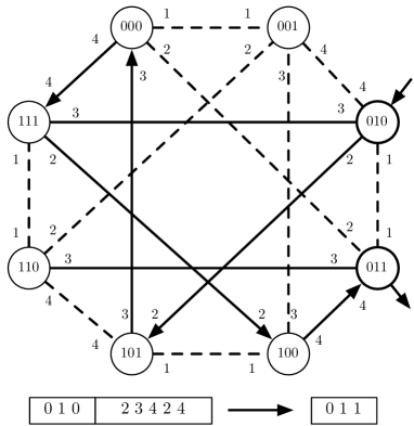
Figure 3: The random-walk symbol-fixing extractor.

The inverter $\mathsf{Inv}$ works as follows: Given an input $x\in[d]^{m}$, $x$ is interpreted as a vertex of $G$. Then $\mathsf{Inv}$ picks $W\in[d]^{n-m}$ uniformly at random. Let $V$ be the unique vertex starting from which the walk described by $W$ ends up in $x$. The inverter outputs $(V,W)$. It is easy to verify that $\mathsf{Inv}$ satisfies the properties of a $0$-inverter.

Now we show that $\mathsf{SFExt}$ is an extractor with the given parameters. We will follow the same line of argument as in the original proof of Kamp and Zuckerman. Let $(v,w)\in[d]^{m}\times[d]^{n-m}$ be a vector sampled from an $(n,k)_{d}$ symbol-fixing source, and let $u:=\mathsf{SFExt}(v,w)$. Recall that $u$ can be seen as the vertex of $G$ reached at the end of the walk described by $w$ starting from $v$. Let $p_{i}$ denote the probability vector corresponding to the walk right after the $i$th step, for $i=0,\ldots,n-m$, and denote by $p$ the uniform probability vector on the vertices of $G$. Our goal is to bound the error $\epsilon$ of the extractor, which is half the $\ell_{1}$ norm of $p_{n-m}-p$.

Suppose that $v$ contains $k_{1}$ random symbols and the remaining $k_{2}:=k-k_{1}$ random symbols are in $w$. Then $p_{0}$ has the value $d^{-k_{1}}$ at $d^{k_{1}}$ of the coordinates and zeros elsewhere, hence

$$\|p_{0}-p\|_{2}^{2} = d^{k_{1}}(d^{-k_{1}}-d^{-m})^{2}+(d^{m}-d^{k_{1}})d^{-2m}$$

$$= d^{-k_{1}}-d^{-m}\leq d^{-k_{1}}.$$

Now for each $i\in[n-m]$, if the $i$th step of the walk corresponds to a random symbol in $w$ the $\ell_{2}$ distance is multiplied by $\lambda_{G}$ by Lemma 21. Otherwise the distance remains the same due to the fact that the labeling of $G$ is consistent. Hence we obtain $\|p_{n-m}-p\|_{2}^{2}\leq d^{-k_{1}}\lambda_{G}^{2k_{2}}$. Translating this into the $\ell_{1}$ norm by using the Cauchy-Schwarz inequality, we obtain $\epsilon$, namely,

$$\epsilon\leq\frac{1}{2}d^{(m-k_{1})/2}\lambda_{G}^{k_{2}}<2^{((m-k_{1})\log d+k_{2}\log\lambda_{G}^{2})/2}.$$

By our assumption, $\lambda_{G}\geq 1/\sqrt{d}$. Hence, everything but $k_{1}$ and $k_{2}$ being fixed, the above bound is maximized when $k_{1}$ is minimized. When $k\leq n-m$, this corresponds to the case $k_{1}=0$, and otherwise to the case $k_{1}=k-n+m$. This gives us the desired upper bound on $\epsilon$. ∎

Combining this with Theorem 19 and setting up the the right asymptotic parameters, we obtain our protocol for the wiretap channel problem.

Corollary 23.

Let $\delta\in[0,1)$ be a constant, and suppose that there is a constructible family of $d$-regular expander graphs with spectral gap at least $1-\lambda$ that is $c$-dense, for constants $\lambda<1$ and $c\geq 1$.

Then, for every large enough $n$, and arbitrarily small constant $\rho>0$, there is a $(\delta n,2^{-\Omega(n)},0)_{d}$-resilient wiretap protocol with block length $n$ and rate

$$R=\left\{\begin{array}[]{ll}1-\delta/\alpha-\rho&\text{if $\delta<\alpha(1-\rho)/(1+\alpha)$,}\\ \alpha/(1+\alpha)-\rho&\text{if $\frac{\alpha(1-\rho)}{1+\alpha}\leq\delta<\frac{\alpha}{1+\alpha}$,}\\ \alpha(1-\delta)-\rho&\text{if $\delta\geq\alpha/(1+\alpha)$,}\\ \end{array}\right.$$ (1)

where $\alpha:=-\log_{d}\lambda^{2}$.

Proof.

For the case $c=1$ we use Theorem 19 with the extractor $\mathsf{SFExt}$ of Theorem 22 and its inverse. Every infinite family of graphs must satisfy $\lambda\geq 2\sqrt{d-1}/d$ [36], and in particular we have $\lambda\geq 1/\sqrt{d}$, as required by Theorem 22 (and $\alpha\leq 1$).

First, we exclude the “intermediate” interval $\alpha(1-\rho)/(1+\alpha)\leq\delta<\alpha/(1+\alpha)$ by observing that we can always increase $\delta$ (at the cost of a lower rate) so that its value falls outside the interval. In particular, in this case, we can increase $\delta$ to $\bar{\delta}:=\alpha/(1+\alpha)$ and apply the result proved later to get a rate $\alpha(1-\bar{\delta})-\rho=\alpha/(1+\alpha)-\rho$. Note that the intermediate interval can be made arbitrarily small by choosing a sufficiently small value for $\rho$.

For the remaining values of $\delta$, we choose the parameters $k:=(1-\delta)n$ and $m:=nR$, where the rate $R$ is chosen according to (1). The parameter $s$ in Theorem 22 can be rewritten as

$$s = \min\{m,n-k\}\log d-\alpha\min\{k,n-m\}\log d$$

$$= \min\{m,\delta n\}\log d-\alpha(n-\max\{m,\delta n\})\log d.$$

Now consider two cases:

1. $\delta<\alpha(1-\rho)/(1+\alpha)$: In this case, we have $R>\delta$ and thus, the value of $s$ simplifies to

   $$s = (\delta-\alpha+\alpha R)n\log d$$

   $$= (\delta-\alpha+\alpha(1-\delta/\alpha-\rho))n\log d$$

   $$= -\alpha\rho n\log d=-\Omega(n).$$

2. $\delta\geq\alpha/(1+\alpha)$: In this case, $R\leq\delta$, and $s$ can be written as

   $$s = (R-\alpha+\alpha\delta)n\log d$$

   $$= (\alpha(1-\delta)-\rho-\alpha+\alpha\delta)n\log d$$

   $$= -\rho n\log d=-\Omega(n).$$

Hence, we always have $s=-\Omega(n)$ and exponentially small error. The case $c>1$ is similar, but involves technicalities for dealing with lack of graphs of arbitrary size in the family. We will elaborate on this in Appendix -F. ∎

Using explicit constructions of Ramanujan graphs that achieve

$$\lambda\leq 2\sqrt{d-1}/d$$

when $d-1$ is a prime power [37, 38, 39], one can obtain $\alpha\geq 1-2/\log d$, which can be made arbitrarily close to one (hence, making the protocol arbitrarily close to the optimal bound) by choosing a suitable alphabet size that does not depend on $n$. Namely, we have the following result:

Corollary 24.

Let $\delta\in[0,1)$ and $\rho>0$ be arbitrary constants. Then, there is a positive integer $d$ only depending on $\rho$ such that the following holds: For every large enough $n$, there is a $(\delta n,2^{-\Omega(n)},0)_{d}$-resilient wiretap protocol with block length $n$ and rate at least $1-\delta-\rho$. ∎

VII Invertible Affine Extractors and Asymptotically Optimal Wiretap Protocols

In this section we will construct a black box transformation for making certain seedless extractors invertible. The method is described in detail for affine extractors, and leads to wiretap protocols with asymptotically optimal rate-resilience trade-offs. Being based on affine extractors, these protocols are only defined for prime power alphabet sizes. On the other hand, the random-walk based protocol discussed in Section VI can be potentially instantiated for an arbitrary alphabet size, though achieving asymptotically sub-optimal parameters (and a positive rate only for an alphabet of size $3$ or more).

Modulo some minor differences, the construction can be simply described as follows: A seedless affine extractor is first used to extract a small number of uniform random bits from the source, and the resulting sequence is then used as the seed for a seeded extractor that extracts almost the entire entropy of the source.

Of course, seeded extractors in general are not guaranteed to work if (as in the above construction) their seed is not independent from the source. However, as observed by Gabizon and Raz [20], a linear seeded extractor can extract from an affine source if the seed is the outcome of an affine extractor on the source. This idea was formalized in a more general setting by Shaltiel [40].

Shaltiel’s result gives a general framework for transforming any seedless extractor (for a family of sources satisfying a certain closedness condition) with short output length to one with an almost optimal output length. The construction uses the imperfect seedless extractor to extract a small number of uniform random bits from the source, and will then use the resulting sequence as the seed for a seeded extractor to extract more random bits from the source. For a suitable choice of the seeded extractor, one can use this construction to extract almost all min-entropy of the source.

The closedness condition needed for this result to work for a family $\mathcal{C}$ of sources is that, letting $f(x,z)$ denote the seeded extractor with seed $z$, for every $\mathcal{X}\in\mathcal{C}$ and every fixed $z$ and $y$, the distribution $(\mathcal{X}|f(\mathcal{X},z)=y)$ belongs to $\mathcal{C}$. If $f$ is a linear function for every fixed $s$, the result will be available for affine sources (since we are imposing a linear constraint on an affine source, it remains an affine source). A more precise statement of Shaltiel’s main result is the following:

Theorem 25.

[40] Let $\mathcal{C}$ be a class of distributions on $\{0,1\}^{n}$ and $f\colon\{0,1\}^{n}\to\{0,1\}^{t}$ be an extractor for $\mathcal{C}$ with error $\epsilon$. Let $F\colon\{0,1\}^{n}\times\{0,1\}^{t}\to\{0,1\}^{m}$ be a function for which $\mathcal{C}$ satisfies the closedness condition above. Then for every $\mathcal{X}\in\mathcal{C}$, $F(\mathcal{X},f(\mathcal{X}))\sim_{\epsilon\cdot 2^{t+3}}F(\mathcal{X},\mathcal{U}_{t})$. ∎

A seeded extractor is called linear if it is a linear function for every fixed choice of the seed. This condition is in particular satisfied by Trevisan’s extractor [41]. For our construction, we will use the following improvement of this extractor due to Raz, Reingold and Vadhan [42]:

Theorem 26.

[42] There is an explicit strong linear seeded $(k,\epsilon)$-extractor $\mathsf{Ext}\colon\mathds{F}_{2}^{n}\times\{0,1\}^{r}\to\mathds{F}_{2}^{m}$ with $r=O(\log^{3}(n/\epsilon))$ and $m=k-O(r)$. ∎

Remark 27.

We note that our arguments would identically work for any other linear seeded extractor as well, for instance those constructed in [43, 44]. However, the most crucial parameter in our application is the output length of the extractor, being closely related to the rate of the wiretap protocols we obtain. Among the constructions we are aware of, the result quoted in Theorem 26 is the best in this regard. Moreover, an affine seeded extractor with better parameters is constructed by Gabizon and Raz [20], but it requires a large alphabet size to work.

Now, having the right tools in hand, we are ready to formally describe our construction of invertible affine extractors with nearly optimal output length. Broadly speaking, the construction follows the abovementioned idea of Shaltiel, Gabizon, and Raz [40, 20] on enlarging the output length of affine extractors, with an additional “twist” for making the extractor invertible. For concreteness, the description is given over the binary field $\mathds{F}_{2}$:

Theorem 28.

For every constant $\delta\in(0,1]$ and every $\alpha\in(0,1)$, there is an explicit $0$-invertible affine extractor $f\colon\mathds{F}_{2}^{n}\to\mathds{F}_{2}^{m}$ for min-entropy $\delta n$ with output length $m=\delta n-O(n^{\alpha})$ and error $\epsilon=O(2^{-n^{\alpha/3}})$.

Proof.

Let $\epsilon:=2^{-n^{\alpha/3}}$, and $t:=O(\log^{3}(n/\epsilon))=O(n^{\alpha})$ be the seed length required by the extractor $\mathsf{Ext}$ in Theorem 26 for input length $n$ and error $\epsilon$, and further, let $n^{\prime}:=n-t$. Set up $\mathsf{Ext}$ for input length $n^{\prime}$, min-entropy $\delta n-t$, seed length $t$ and error $\epsilon$. Also set up Bourgain’s extractor $\mathsf{AExt}$ (Theorem 12) for input length $n^{\prime}$ and entropy rate $\delta^{\prime}$, for an arbitrary constant $\delta^{\prime}<\delta$. Then the function $f$ will view the $n$-bit input sequence as a tuple $(s,x)$, $s\in\mathds{F}_{2}^{t}$ and $x\in\mathds{F}_{2}^{n^{\prime}}$, and outputs $\mathsf{Ext}(x,s+\mathsf{AExt}(x)|_{[t]})$. This is depicted in Fig. 4.

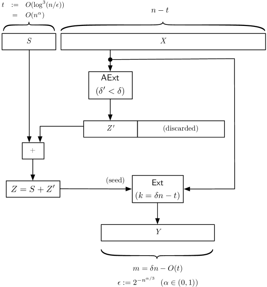
Figure 4: Construction of the invertible affine extractor.

First we show that the construction gives an affine extractor. Suppose that $(S,X)\in\mathds{F}_{2}^{t}\times\mathds{F}_{2}^{n^{\prime}}$ is a random variable sampled from an affine distribution with min-entropy $\delta n$. The variable $S$ can have an affine dependency on $X$. Hence, for every fixed $s\in\mathds{F}_{2}^{t}$, the distribution of $X$ conditioned on the event $S=s$ is affine with min-entropy at least $\delta n-t$, which is at least $\delta^{\prime}n^{\prime}$ for large enough $n$. Hence $\mathsf{AExt}(X)$ will be $2^{-\Omega(n)}$-close to uniform by Theorem 12. This implies that $\mathsf{AExt}(X)|_{[t]}+S$ can extract $t$ random bits from the affine source with error $2^{-\Omega(n)}$. Combining this with Theorem 25, and noticing the fact that the class of affine extractors is closed with respect to linear seeded extractors, we conclude that $f$ is an affine extractor with error at most $\epsilon+2^{-\Omega(n)}\cdot 2^{t+3}=O(2^{-n^{\alpha/3}})$.

Now the inverter works as follows: Given $y\in\mathds{F}_{2}^{m}$, first it picks $Z\in\mathds{F}_{2}^{t}$ uniformly at random. The seeded extractor $\mathsf{Ext}$, given the seed $Z$ is a linear function $\mathsf{Ext}_{Z}\colon\mathds{F}_{2}^{n^{\prime}}\to\mathds{F}_{2}^{m}$. Without loss of generality, assume that this function is surjective. Then the inverter picks $X\in\mathds{F}_{2}^{n^{\prime}}$ uniformly at random from the affine subspace defined by the linear constraint $\mathsf{Ext}_{Z}(X)=y$, and outputs $(Z+\mathsf{AExt}(X)|_{[t]},X)$. It is easy to verify that the output is indeed a valid preimage of $y$. To see the uniformity of the inverter, note that if $y$ is chosen uniformly at random, the distribution of $(Z,X)$ will be uniform on $\mathds{F}_{2}^{n}$. Hence $(Z+\mathsf{AExt}(X)|_{[t]},X)$, which is the output of the inverter, will be uniform. ∎

In the above construction we are using an affine and a linear seeded extractor as black boxes, and hence, they can be replaced by any other extractors as well (the construction will achieve an optimal rate provided that the seeded extractor extracts almost the entire source entropy). In particular, over large fields one can use the affine and seeded extractors given by Gabizon and Raz [20] that work for sub-constant entropy rates as well.

Moreover, for concreteness we described and instantiated our construction over the binary field. Observe that Shaltiel’s result, for the special case of affine sources, holds regardless of the alphabet size. Moreover, Trevisan’s linear seeded extractor can be naturally extended to handle arbitrary alphabets. Hence, in order to extend our result to non-binary alphabets, it suffices to ensure that a suitable seedless affine extractor that supports the desired alphabet size is available. Bourgain’s original result [21] is stated and proved for the binary alphabet; however, this result can be adapted to work for larger fields as well [45]. Such an extension (along with some improvements and simplifications) is made explicit by Yehudayoff [22].

An affine extractor is in particular, a symbol-fixing extractor. Hence Theorem 28, combined with Theorem 19 gives us a wiretap protocol with almost optimal parameters:

Theorem 29.

Let $\delta\in[0,1)$ and $\alpha\in(0,1/3)$ be constants. Then for a prime power $q>1$ and every large enough $n$ there is a $(\delta n,O(2^{-n^{\alpha}}),0)_{q}$-resilient wiretap protocol with block length $n$ and rate $1-\delta-o(1)$. ∎

VIII Further Applications and Extensions

In this section we will sketch some important applications of our technique to more general wiretap problems.

VIII-A Noisy Channels and Active Intruders

Suppose that Alice wants to transmit a particular sequence to Bob through a noisy channel. She can use various techniques from coding theory to encode her information and protect it against noise. Now what if there is an intruder who can partially observe the transmitted sequence and even manipulate it? Modification of the sequence by the intruder can be regarded in the same way as the channel noise; thus one gets security against active intrusion as a “bonus” by constructing a code that is resilient against noise and passive eavesdropping. There are two natural and modular approaches to construct such a code.

A possible attempt would be to first encode the message using a good error-correcting code and then to apply a wiretap encoder to protect the encoded sequence against the wiretapper. However, this will not necessarily keep the information protected against the channel noise, as the combination of the wiretap encoder and decoder does not have to be resistant to noise.

Another attempt is to first use a wiretap encoder and then apply an error-correcting code on the resulting sequence. Here it is not necessarily the case that the information will be kept secure against intrusion anymore, as the wiretapper now gets to observe the bits from the channel-encoded sequence that may reveal information about the original sequence. However, the wiretap protocol given in Theorem 29 is constructed from an invertible affine extractor, and guarantees resiliency even if the intruder is allowed to observe arbitrary linear combinations of the transmitted sequence (in this case, the distribution of the encoded sequence subject to the intruder’s observation becomes an affine source and thus, the arguments of the proof of Theorem 19 remain valid). In particular, Theorem 29 holds even if the intruder’s observation is allowed to be obtained after applying any arbitrary linear mapping on the output of the wiretap encoder. Hence, we can use the wiretap scheme as an outer code and still ensure privacy against an active intruder and reliability in presence of a noisy channel, provided that the error-correcting code being used as the inner code is linear. This immediately gives us the following result:

Theorem 30.

Suppose that there is a $q$-ary linear error-correcting code with rate $R$ that is able to correct up to a $\tau$ fraction of errors (via unique or list decoding). Then for every constant $\delta\in[0,1)$ and $\alpha\in(0,1/3)$ and large enough $n$, there is a $(\delta n,O(2^{-n^{\alpha}}),0)_{q}$-resilient wiretap protocol with block length $n$ and rate $R-\delta-o(1)$ that can also correct up to a $\tau$ fraction of errors.

Proof.

We use the wiretap code given by Theorem 29 as the outer code and the linear channel code with rate $R$ as the inner code. Suppose that the rate of the outer code is $R^{\prime}$ and the block length of the combined code is $n$. By the discussion above and using Theorem 29, the combined code tolerates against $Rn(1-R^{\prime}-o(1))$ bits of observation by the intruder, even after linear post-processings of the inner code. Therefore the resilience of the combined code can be written as

$$\delta=R(1-R^{\prime}-o(1)),$$

from which we can compute the rate of the combined code as

$$RR^{\prime}=R-\delta-o(1).$$

∎

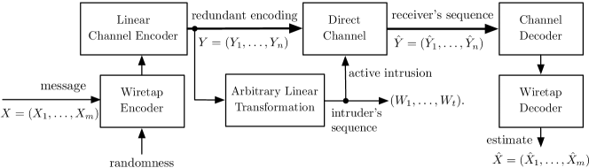
Figure 5: Wiretap scheme composed with channel coding. If the wiretap scheme is constructed by an invertible affine extractor, it can guarantee secrecy even in presence of arbitrary linear manipulation of the information. Active intrusion can be defied using an error-correcting inner code.

The setting discussed above is shown in Fig. 5. The same idea can be used to protect fountain codes, e.g., LT- [46] and Raptor Codes [47], against wiretappers without affecting the error correction capabilities of the code.

Obviously this simple composition idea can be used for any type of channel so long as the inner code is linear, at the cost of reducing the total rate by almost $\delta$ (following exactly the same argument as in Theorem 30). Hence, if the inner code achieves the Shannon capacity of the direct channel (in the absence of the wiretapper), the composed code will have a rate that is smaller than the direct channel capacity by the resilience parameter $\delta$. This is known to be the best possible rate when the channels are discrete, memoryless, and symmetric and the wiretap channel is a degraded version of the symmetric channel [48, 49].

VIII-B Network Coding

Our wiretap protocol from invertible affine extractors is also applicable in the more general setting of transmission over networks. In this work we focus on a network setting known as multicast. A multicast communication network can be modeled as a directed graph, in which nodes represent the network devices and information is transmitted along the edges. One particular node is identified as the source and $m$ nodes are identified as receivers. The main problem in network coding is to have the source reliably transmit information to the receivers at the highest possible rate, while allowing the intermediate nodes arbitrarily process the information along the way.

Suppose that, in the graph that defines the topology of the network, the min-cut between the source to each receiver is $n$. It was shown in [50] that the source can transmit information up to rate $n$ (symbols per transmission) to all receivers (which is optimal), and in [51, 52] that linear network coding is in fact sufficient to achieve this rate. That is, the transmission at rate $n$ is possible when the intermediate nodes are allowed to forward packets that are (as symbols over a finite field) linear combinations of the packets that they receive (See [53] for a comprehensive account of these and other relevant results).

A basic example is shown by the butterfly network in Fig. 6. This network consists of a source on the top and two receivers on the bottom, where the min-cut to each receiver is $2$. Without processing the incoming data, as in the left figure, one of the two receivers may receive information at the optimal rate of $2$ symbols per transmission (namely, receiver $1$ in the figure). However, due to the bottleneck existing in the middle (shown by the thick edge $a\to b$), the other receiver will be forced to receive at an inferior rate of $1$ symbol per transmission. However, if linear processing of the information is allowed, node $a$ may combine its incoming information by treating packets as symbols over a finite field and adding them up, as in the right figure. Both receivers may then solve a full-rank system of linear equations to retrieve the original source symbols $x_{1}$ and $x_{2}$, and thereby achieve the optimal min-cut rate.

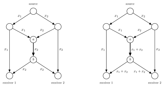
Figure 6: Network coding (right), versus unprocessed forwarding (left).

Designing wiretap protocols for networks is an important question in network coding, which was first posed by Cai and Yeung [11]. In this problem, an intruder can choose a bounded number, say $t$, of the edges and eavesdrop all the packets going through those edges. They designed a network code that could provide the optimal multicast rate of $n-t$ with perfect privacy. However this code requires an alphabet size of order $\binom{|E|}{t}$, where $E$ is the set of edges. Their result was later improved in [54] who showed that a random linear coding scheme can provide privacy with a much smaller alphabet size if one is willing to achieve a slightly sub-optimal rate. Namely, they obtain rate $n-t(1+\epsilon)$ with an alphabet of size roughly $\mathrm{\Theta}(|E|^{1/\epsilon})$, and show that achieving the exact optimal rate is not possible with small alphabet size.

El Rouayheb and Soljanin [55] suggested to use the original code of Ozarow and Wyner [2] as an outer code at the source and showed that a careful choice of the network code can provide optimal rate with perfect privacy. However, their code eventually needs an alphabet of size at least $\binom{|E|-1}{t-1}+m$. Building upon this work, Silva and Kschischang [8] constructed an outer code that provides similar results while leaving the underlying network code unchanged. However, their result comes at the cost of increasing the packet size by a multiplicative factor of at least the min-cut bound, $n$ (or in mathematical terms, the original alphabet size $q$ of the network is enlarged to at least $q^{n}$). For practical purposes, this is an acceptable solution provided that an estimate on the min-cut size of the network is available at the wiretap encoder.

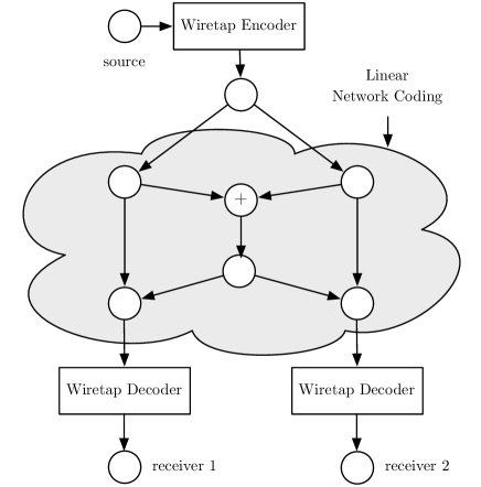
Figure 7: Linear network coding with an outer layer of wiretap encoding added for providing secrecy.

By the discussion presented in Section VIII-A, the rate-optimal wiretap protocol given in Theorem 29 stays resilient even in presence of any linear post-processing of the encoded information. Thus, using the wiretap encoder given by this result as an outer-code in the source node, one can construct an asymptotically optimal wiretap protocol for networks that is completely unaware of the network and eliminates all the restrictions in the above results. This is schematically shown in Fig. 7. Hence, extending our notion of $(t,\epsilon,\gamma)_{q}$-resilient wiretap protocols naturally to communication networks, we obtain the following:

Theorem 31.

Let $\delta\in[0,1)$ and $\alpha\in(0,1/3)$ be constants, and consider a network that uses a linear coding scheme over a finite field $\mathds{F}_{q}$ for reliably transmitting information at rate $R$. Suppose that, at each transmission, an intruder can arbitrarily observe up to $\delta R$ intermediate links in the network. Then the source and the receiver nodes can use an outer code of rate $1-\delta-o(1)$ (obtaining a total rate of $R(1-\delta)-o(1)$) which is completely independent of the network, leaves the network code unchanged, and provides almost perfect privacy with error $O(2^{-{R}^{\alpha}})$ and zero leakage over a $q$-ary alphabet. ∎

In addition to the above result that uses the invertible affine extractor of Theorem 28, it is possible to use other rate-optimal invertiable affine extractors. In particular, observe that the restricted affine extractor of Theorem 14 (and in particular, Corollary 15) is a linear function (over the extension field) and is thus, obviously has an efficient $0$-inverter (since inverting the extractor amounts to solving a system of linear equations). By using this extractor (instantiated with Gabidulin’s MRD codes as in Corollary 15), we may recover the result of Silva and Kschischang [8] in our framework. More precisely, we have the following result:

Corollary 32.

Let $q$ be any prime power, and consider a network with minimum cut of size $n$ that uses a linear coding scheme over $\mathds{F}_{q}$ for reliably transmitting information at rate $R$. Suppose that, at each transmission, an intruder can arbitrarily observe up to $\delta R$ intermediate links in the network, for some $\delta\in[0,1)$. Then the source and the receiver nodes can use an outer code of rate $1-\delta$ over $\mathds{F}_{q^{n}}$ (obtaining a total rate of $R(1-\delta)$) that provides perfect privacy over a $q^{n}$-ary alphabet. ∎

VIII-C Arbitrary Processing

In this section we consider the erasure wiretap problem in its most general setting, which is still of practical importance. Suppose that the information emitted by the source goes through an arbitrary communication medium and is arbitrarily processed on the way to provide protection against noise, to obtain better throughput, or for other reasons. Now consider an intruder who is able to eavesdrop a bounded amount of information at various points of the channel. One can model this scenario in the same way as the original point-to-point wiretap channel problem (depicted in Fig. 1), with the difference that instead of observing $t$ arbitrarily chosen bits, the intruder now gets to choose an arbitrary Boolean circuit $\mathcal{C}$ with $t$ output bits (which captures the accumulation of all the intermediate processing) and observes the output of the circuit when applied to the transmitted sequence.

Obviously there is no way to guarantee resiliency in this setting, since the intruder can simply choose $\mathcal{C}$ to compute $t$ output bits of the wiretap decoder. However, suppose that in addition there is an auxiliary communication channel between the source and the receiver (that we call the side channel) that is separated from the main channel, and hence, the information passed through the two channel do not blend together by the intermediate processing.

We call this scenario, shown in Fig. 8, the general wiretap problem and extend our notion of $(t,\epsilon,\gamma)$-resilient protocol to this problem. The slight modification in the generalized notion is that now the output of the encoder (and the input of the decoder) is a pair of strings $(Y_{1},Y_{2})\in\{0,1\}^{n}\times\{0,1\}^{n^{\prime}}$, where $Y_{1}$ (resp., $Y_{2}$) is sent through the main (resp., side) channel. Now we call $n+n^{\prime}$ the block length and let the intruder choose an arbitrary Boolean function $\mathcal{C}\colon\{0,1\}^{n}\to\{0,1\}^{t}$, and observe $(\mathcal{C}(Y_{1}),Y_{2})$.

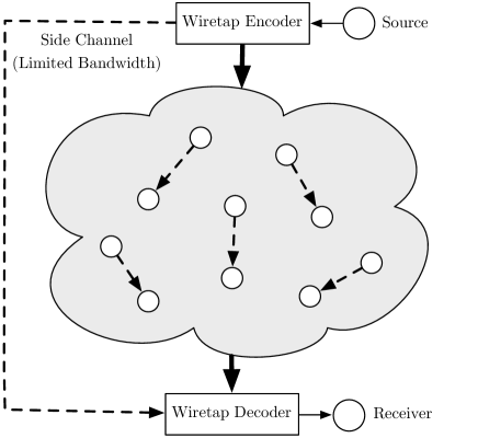
Figure 8: The wiretap channel problem in presence of arbitrary intermediate processing. In this example, data is transmitted over a packet network (shown as a cloud) in which some intermediate links (showed by the dashed arrows), as well as the side channel (also dashed), are accessible to an intruder.

More precisely, the generalized model that we consider can be described as follows:

1. A wiretap encoder $E(X,Z)$ encodes a message $X\in\{0,1\}^{m}$ using a uniformly random seed $Z$. The output of the encoder is a pair of strings $(Y_{1},Y_{2})$.

2. The encoded strings $Y_{1}$ and $Y_{2}$ are sent through the main channel and the side channel, respectively.

3. The intruder chooses an arbitrary function $\mathcal{C}\colon\{0,1\}^{n}\to\{0,1\}^{t}$, and observes $(\mathcal{C}(Y_{1}),Y_{2})$.

4. A wiretap decoder $D(Y_{1},Y_{2})$ receives the encoded strings $(Y_{1},Y_{2})$ and reconstructs the message $X$.

For a pair of strings $(w_{1},w_{2})\in\{0,1\}^{t}\times\{0,1\}^{n^{\prime}}$, denote by $\mathcal{X}_{(w_{1},w_{2})}$ the distribution of the message $X$ conditioned on the event $(\mathcal{C}(Y_{1}),Y_{2})=(w_{1},w_{2})$. Now we call a generalized wiretap encoder/decoder pair $(t,\epsilon,\gamma)$-resilient if, for every choice of the function $\mathcal{C}$ chosen by the intruder, the following holds. Similar to Definition 4, denote by $B_{\mathcal{C}}$ the set of bad observations

$$B_{\mathcal{C}}:=\{(w_{1},w_{2})\in\{0,1\}^{t}\times\{0,1\}^{n^{\prime}}\colon{\mathsf{dist}}(X,\mathcal{X}_{(w_{1},w_{2})})>\epsilon\}.$$

Then the wiretap protocol must satisfy

$$\Pr[(\mathcal{C}(Y_{1}),Y_{2})\in B_{\mathcal{C}}]\leq\gamma.$$

The parameters $\epsilon$ and $\gamma$ are again called the error and the leakage of the protocol. The rate and resilience parameters are now given by $R:=m/(n+n^{\prime})$ and $\delta:=t/n$, respectively.

The standard definition of wiretap protocols (Definition 4) corrsponds to the case when $\mathcal{C}(Y_{1})=Y_{1}|_{S}$, for some $S\subseteq[n]$, and $Y_{2}$ is the empty string. Since the information in $Y_{2}$, transmitted through the side channel, does not affect the resilience parameter and only lowers the rate, we see that the information-theoretic upper bound for the achievable rates in the original wiretap problem (namely, $R\leq 1-\delta+o(1)$) extends to the generalized wiretap problem as well. Below we show that for the generalized problem, secure transmission is indeed possible at asymptotically optimal rates (that is, $R\geq 1-\delta-o(1)$).

As before, our idea is to use invertible extractors to construct general wiretap protocols, but this time we use invertible strong seeded extractors. Strong seeded extractors were used in [10] to construct ERFs, and this is exactly what we use as the decoder in our protocol. As the encoder we will use the corresponding inverter, which outputs a pair of strings, one for the extractor’s input which is sent through the main channel and another as the seed which is sent through the side channel. Hence we will obtain the following result:

Theorem 33.

Let $\delta\in[0,1)$ be a constant. Then for every $\alpha,\epsilon>0$, there is a $(\delta n,\epsilon,2^{-\alpha n}+\epsilon)$-resilient wiretap protocol for the general wiretap channel problem that sends $n$ bits through the main channel and $n^{\prime}=O(\log^{3}(n/\epsilon^{2}))$ bits through the side channel and achieves rate $1-\delta-\alpha-O(n^{\prime}/(n+n^{\prime}))$. The protocol is secure even when the entire communication through the side channel is observable by the intruder.

Proof.

We will need the following claim in our proof, which is easy to verify using an averaging argument:

Claim.

Let $f\colon\{0,1\}^{n}\to\{0,1\}^{\delta n}$ be any Boolean function. Then for every $\alpha>0$, and $X\sim\mathcal{U}_{n}$, the probability that $f(X)$ has fewer than $2^{n(1-\delta-\alpha)}$ preimages is at most $2^{-\alpha n}$.

Proof of Claim.

Define

$$B:=\{y\in\{0,1\}^{m}\colon|f^{-1}(y)|<2^{n(1-\delta-\alpha)}\}.$$

Thus, the probability that we wish to bound is

$$\Pr_{X}[f(X)\in B] = 2^{-n}\sum_{y\in B}|f^{-1}(y)|$$

$$< 2^{-n}\sum_{y\in B}|f^{-1}(y)|2^{n(1-\delta-\alpha)}<2^{-\alpha},$$

where the last inequality is from the trivial bound $|B|\leq 2^{\delta n}$. ∎

Now, let $\mathsf{Ext}$ be the linear seeded extractor of Theorem 26, set up for input length $n$, seed length $n^{\prime}=O(\log^{3}(n/\epsilon^{2}))$, min-entropy $n(1-\delta-\alpha)$, output length $m=n(1-\delta-\alpha)-O(n^{\prime})$, and error $\epsilon^{2}$. Then the encoder chooses a seed $Z$ for the extractor uniformly at random and sends it through the side channel.

For the chosen value of $Z$, the extractor is a linear function, and as before, given a message $X\in\{0,1\}^{m}$, the encoder picks a random vector $Y$ in the affine subspace that is mapped by this linear function to $X$ and sends it through the public channel. By Remark 18, the encoder is polynomial-time computable and $Y$ is uniformly distributed on $\{0,1\}^{n}$.

The decoder, upon receiving $(Y,Z)$, applies the extractor to the seed $Z$ received through the side channel and the transmitted string $Y$. This obviously reproduces the sent message $X=\mathsf{Ext}(Y,Z)$. The resiliency of the protocol can be shown in a similar manner as in Theorem 19, as follows. Suppose that the intruder observes the seed $Z$ and $W:=\mathcal{C}(Y)\in\{0,1\}^{\delta n}$, for an arbitrary function $\mathcal{C}\colon\{0,1\}^{n}\to\{0,1\}^{\delta n}$.

First, note that by the above claim, with probability at least $1-2^{-\alpha n}$, the string $Y$ transmitted through the main channel, conditioned on the observation $W$ of the intruder from the main channel, has a distribution $\mathcal{Y}$ with min-entropy at least $n(1-\delta-\alpha)$. Call a particular realization $w\in\{0,1\}^{\delta n}$ of the observation outcome $W$ good if it makes $\mathcal{Y}$ satisfies this property. In the sequel, we condition the random variable $W$ to a good outcome $w$.

Now suppose that the seed $Z$ is entirely revealed to the intruder, and let $z\in\{0,1\}^{n^{\prime}}$ denote the particular realization of $Z$. By an averaging argument, with probability at least $1-\epsilon$, $Z$ is a good seed for $\mathcal{Y}$, in the sense that $\mathsf{Ext}(\mathcal{Y},z)$ is $\epsilon$-close to uniform.

Therefore, conditioned on the event that both parts of the observation outcome $(w,z)$ are good, the message distribution conditioned on the intruder’s observation (which is given by $\mathsf{Ext}(\mathcal{Y},z)$) is $\epsilon$-close to uniform. The leakage parameter is given by the probability that either the part of the observation outcome corresponding to the main channel or the part corresponding to the side channel is not good. By a union bound this probability is upper bounded by $2^{-\alpha n}+\epsilon$, which completes the proof of resiliency. ∎

We observe that it is not possible to guarantee zero leakage for the general wiretap problem above. As an extreme case, suppose that the function $\mathcal{C}$ is chosen in a way that it has a single preimage for a particular output $w$ (i.e., $|\mathcal{C}^{-1}(w)|=1$). With nonzero probability the observation of the intruder from the main channel may turn out to be $w$, in which case the entire message is revealed (since the intruder learns the entire communication $(Y_{1},Y_{2})$ in this case). Nevertheless, it is possible to guarantee negligible leakage as the above theorem does.

Finally, we remark that the general protocol above can be used for the original wiretap II problem (where there is no intermediate processing involved). In this case, both encoded strings $Y_{1}$ and $Y_{2}$ are sent through the main channel (since in the original problem there is no side channel). But fortunately, since the intruder’s function $\mathcal{C}$ is a simple projection (in particular, $\mathcal{C}(Y_{1})=Y_{1}|_{S}$ for a small set of the coordinate positions $S\subseteq[n]$), sending both $Y_{1}$ and $Y_{2}$ through the same channel for this special case does not affect the secrecy guarantees of the generalized wiretap model. Contrary to Theorem 29 however, we cannot guarantee zero leakage when we use a generalized wiretap protocol for the original wiretap II model.

-D Review of the Related Notions in Cryptography

In this appendix we review notions in cryptography that are relevant to our wiretap protocol model introduced in Section III. These notions include resilient functions (RF) and almost perfect resilient functions (APRF), exposure-resilient functions (ERF), and all-or-nothing transforms (AONT).

The notion of resilient functions was introduced in [56] (and also [57] as the bit-extraction problem). A deterministic polynomial-time computable function $f\colon\{0,1\}^{n}\to\{0,1\}^{m}$ is called $t$-resilient if whenever any $t$ bits of the its input are arbitrarily chosen by an adversary and the rest of the bits are chosen uniformly at random, then the output distribution of the function is (close to) uniform. APRF is a stronger variation where the criterion for uniformity of the output distribution is defined with respect to the $\ell_{\infty}$ (i.e., point-wise distance of distributions) rather than $\ell_{1}$. This stronger requirement allows for an “adaptive security” of APRFs.

ERFs, introduced in [10], are similar to resilient functions except that the entire input is chosen uniformly at random, and the view of the adversary from the output remains (close to) uniform even after observing any $t$ input bits of his choice. More formally, a polynomial-time computable function $f\colon\{0,1\}^{n}\to\{0,1\}^{m}$ is a $t$-ERF if for a uniform random variable $Y$ on $\mathds{F}_{2}^{n}$ and all $S\subseteq[n]$ such that $|S|\leq t$, the two distributions $(Y|_{S},f(Y))$ and $(Y|_{S},\mathcal{U}_{m})$ are close in statistical distance. As such, ERFs are slightly weaker than resilient functions since their output is fully random subject to a random fixing of positions in $S$, as opposed to all possible fixings. A variation of ERF called adaptive ERF allows the adversary to make up to $t$ adaptive queries to the input; i.e., the choice of each query position may depend on the outcome of the previous ones. Adaptive ERFs turn out to be much more challenging to construct than ERFs.

ERFs and resilient functions are known to be useful in a scenario similar to the wiretap channel problem. Suppose that Alice and Bob want to agree on any random string (for example to use as a session key) and that their communication channel is wiretapped. In this case Alice can send a random string $Y\in\{0,1\}^{n}$ to Bob and then the two parties agree on $X:=f(Y)$, where $f$ is a $t$-ERF or a $t$-resilient function. It follows that an intruder who observes any $t$ positions of $Y$ does not learn much about the agreed string $X$. The main difference between this setting and the model we introduced in Definition 4 is that the two parties only care about the fact that $X$ is uniformly random, and not its actual realization. That is, we have a secure agreement problem rather than a secure communication problem.

Another closely related notion is that of all-or-nothing transforms, which was suggested in [15] for protection of block ciphers. This notion is defined as follows.

Definition 34.

A randomized polynomial-time computable function $f\colon\{0,1\}^{m}\times\{0,1\}^{r}\to\{0,1\}^{n}$, $(m\leq n,r={\mathsf{poly}}(n))$, where the first argument is the function’s input and the second one is a random seed, is called a (statistical, non-adaptive, and secret-only) $t$-AONT with error $\epsilon$ if

1. It is efficiently invertible. That is, there is a deterministic polynomial time algorithm $A$ such that for every $x\in\{0,1\}^{m}$, we have $\Pr_{Z\sim\mathcal{U}_{r}}[A(f(x,Z))=x]=1$.

2. For every $S\subseteq[n]$ such that $|S|\leq t$, and all $x_{1},x_{2}\in\{0,1\}^{m}$ we have that the two distributions $f(x_{1},\mathcal{U}_{r})|_{S}$ and $f(x_{2},\mathcal{U}_{r})|_{S}$ are $\epsilon$-close.

An AONT with $\epsilon=0$ is called perfect. It is easy to see that perfectly private wiretap protocols are equivalent to perfect adaptive AONTs. It was shown in [12] that such functions can not exist (with positive, constant rate) when the adversary is allowed to observe more than half of the encoded bits (so this is a too strong notion for the wiretap channel problem). A similar negative result was obtained in [13] for the case of perfect linear RFs.

As pointed out in [12], AONTs can be used in the original scenario of Ozarow and Wyner’s wiretap channel problem. However, the best known constructions of AONTs (over small alphabets) can achieve rate-resilience trade-offs that are far from the information-theoretic optimum (see Figure 2). Moreover it is straightforward to see that, in the perfectly private wiretap coding scheme of Ozarow and Wyner [2], the encoder can be seen as an adaptively secure, perfect AONTs and the decoder is in fact an adaptive perfect RF.

While an AONT requires indistinguishability of intruder’s view for every fixed pair $(x_{1},x_{2})$ of messages, the relaxed notion of average-case AONT requires the expected distance of $f(x_{1},\mathcal{U}_{r})|_{S}$ and $f(x_{2},\mathcal{U}_{r})|_{S}$ to be at most $\epsilon$ for a uniform random message pair. That is, for average-case AONTs, the second condition in Definition 34 is relaxed to

$$\mathbb{E}_{X_{1},X_{2}\sim\mathcal{U}_{m}}[{\mathsf{dist}}(f(X_{1},\mathcal{U}_{r})|_{S},f(X_{2},\mathcal{U}_{r})|_{S}]\leq\epsilon.$$

Hence, for a negligible $\epsilon$, the distance will be negligible for all but a negligible fraction of message pairs. Here we show that, up to a loss in parameters, wiretap protocols are equivalent to average case AONTs:

Lemma 35.

Let $(E,D)$ be an encoding/decoding pair for a $(t,\epsilon,\gamma)_{2}$-resilient wiretap protocol. Then $E$ is an average-case $t$-AONT with error at most $2(\epsilon+\gamma)$.

Conversely, an average-case $t$-AONT with error $\eta^{4}$ (for some small $\eta<1/2$) can be used as a $(t,2\eta,2\eta)$-resilient wiretap encoder.

Proof.

Consider a $(t,\epsilon,\gamma)_{2}$-resilient wiretap protocol as in Definition 4, and accordingly, let the random variable $Y=E(X,Z)$ denote the encoding of $X$ with a random seed $Z$. For a set $S\subseteq[n]$ of size at most $t$, denote by $W:=Y|_{S}$ the intruder’s observation.

The resiliency condition implies that, the set of bad observations $B_{S}$ has a probability mass of at most $\gamma$ and hence, the expected distance ${\mathsf{dist}}(X|W,X)$ taken over the distribution of $W$ is at most $\epsilon+\gamma$. Now we can apply Proposition 37 in the appendix to the jointly distributed pair of random variables $(W,X)$, and conclude that the expected distance ${\mathsf{dist}}(W|X,W)$ over the distribution of $X$ (which is uniform) is at most $\epsilon+\gamma$. This implies that the encoder is an average-case $t$-AONT with error at most $2(\epsilon+\gamma)$.

For the converse, we define the wiretap encoder $E$ and decoder $D$ by the AONT and its inverse, respectively. From the definition of AONTs, it is immediately clear that the decodability condition of Definition 4 is satisfied. In order to show the resiliency, fix any subset $S\subseteq[n]$ of size $t$ and assume that the intruder observes $W:=Y|_{S}$, where $Y$ is the encoding of a random message $X\in\{0,1\}^{m}$. Denote by $\mathcal{W}$ the distribution of $W$ on $\{0,1\}^{t}$, and for every $x\in\{0,1\}^{m}$, by $\mathcal{W}_{x}$ the distribution of $W$ conditioned on the event $X=x$. Now, the definition of $t$-AONT implies that for a random pair $X_{1},X_{2}\sim\mathcal{U}_{m}$, we have

$$\mathbb{E}_{X_{1},X_{2}}{\mathsf{dist}}(\mathcal{W}_{X_{1}},\mathcal{W}_{X_{2}})\leq\eta^{4}.$$

Fix any $\hat{x}\in\{0,1\}^{m}$ for which we have

$$\mathbb{E}_{X}{\mathsf{dist}}(\mathcal{W}_{\hat{x}},\mathcal{W}_{X})\leq\eta^{4}.$$

By averaging, we know that such an $\hat{x}$ exists. By another averaging argument (using Markov’s inequality), there is a subset $\mathcal{G}\subseteq\{0,1\}^{m}$ of size at least $(1-\eta^{2})2^{m}$ such that for every $x\in\mathcal{G}$, we have ${\mathsf{dist}}(\mathcal{W}_{\hat{x}},\mathcal{W}_{x})\leq\eta^{2}$. Therefore, for each $x\in\mathcal{G}$, the distribution $\mathcal{W}_{x}$ (now seen as a vector of probabilities over $\{0,1\}^{t}$), can be written as $\mathcal{W}_{x}=\mathcal{W}_{\hat{x}}+\mathcal{E}_{x}$, where by the definition of statistical distance, the $\ell_{1}$ norm $\|\mathcal{E}_{x}\|_{1}$ is at most $2\eta^{2}$. On the other hand, we can write down the convex combination

$$\mathcal{W} = 2^{-m}\sum_{x\in\{0,1\}^{m}}\mathcal{W}_{x}$$

$$= 2^{-m}\sum_{x\in\mathcal{G}}\mathcal{W}_{x}+2^{-m}\sum_{x\in\{0,1\}^{m}\setminus\mathcal{G}}\mathcal{W}_{x}$$

$$= 2^{-m}\sum_{x\in\mathcal{G}}\mathcal{W}_{x}+\mathcal{E},$$

where we have defined $\mathcal{E}:=2^{-m}\sum_{x\in\{0,1\}^{m}\setminus\mathcal{G}}\mathcal{W}_{x}$, and know that $\|\mathcal{E}\|_{1}\leq\eta^{2}$. Substituting for $\mathcal{W}_{x}$, we get

$$\mathcal{W} = 2^{-m}\sum_{x\in\mathcal{G}}(\mathcal{W}_{\hat{x}}+\mathcal{E}_{x})+\mathcal{E}$$

$$= 2^{-m}|\mathcal{G}|\mathcal{W}_{\hat{x}}+\mathcal{E}^{\prime},$$

where $\mathcal{E}^{\prime}:=2^{-m}\sum_{x\in\mathcal{G}}\mathcal{E}_{x}+\mathcal{E}$. By the bounds on the $\ell_{1}$ norm on the $\mathcal{E}_{x}$, we know that $\|\mathcal{E}^{\prime}\|_{1}\leq 3\eta^{2}$, which implies

$$\|\mathcal{W}-2^{-m}|\mathcal{G}|\mathcal{W}_{\hat{x}}\|_{1}\leq 3\eta^{2}.$$ (2)

Now, since $2^{-m}|G|\geq 1-\eta^{2}$, we have

$$\|\mathcal{W}-\mathcal{W}_{\hat{x}}\|_{1}\leq\|\mathcal{W}-2^{-m}|\mathcal{G}|\mathcal{W}_{\hat{x}}\|_{1}+\eta^{2}\leq 4\eta^{2},$$

where the second inequality is from (2). So, the distributions $\mathcal{W}$ and $\mathcal{W}_{\hat{x}}$ are $(2\eta^{2})$-close. Now we can apply Proposition 37 for the joint distribution of the variables $(X,W)$, and deduce

$$\mathbb{E}_{W}[{\mathsf{dist}}(X|W,\mathcal{U}_{m})]=\mathbb{E}_{X}[{\mathsf{dist}}(\mathcal{W}_{X},\mathcal{W})].$$ (3)

Here we have used the notation $X|W$ for the distribution of the random variable $X$ conditioned on the observation $W$. We know that for every $x\in\mathcal{G}$,

$${\mathsf{dist}}(\mathcal{W}_{x},\mathcal{W})\leq{\mathsf{dist}}(\mathcal{W}_{x},\mathcal{W}_{\hat{x}})+2\eta^{2}\leq 3\eta^{2}.$$

Thus,

$$\mathbb{E}_{X}[{\mathsf{dist}}(\mathcal{W}_{X},\mathcal{W})]\leq|\{0,1\}^{m}\setminus\mathcal{G}|2^{-m}+3\eta^{2}\leq 4\eta^{2}.$$

Combined with (3), we get

$$\mathbb{E}_{W}[{\mathsf{dist}}(X|W,\mathcal{U}_{m})]\leq 4\eta^{2}.$$

Now we are ready to apply Markov’s inequality again to conclude that

$$\Pr[{\mathsf{dist}}(X|W,\mathcal{U}_{m})>2\eta]\leq 2\eta,$$

which proves the resiliency condition. ∎

It is important to note that the converse direction does not guarantee zero leakage, and hence, zero leakage wiretap protocols are in general stronger than average-case AONTs. An average-case to worst-case reduction for AONTs was shown in [10] which, combined with the above lemma, can be used to show that any wiretap protocol can be used to construct an AONT (at the cost of a rate loss).

A simple universal transformation was proposed in [10] to obtain an AONT from any ERF, by one-time padding the message with a random string obtained from the ERF. In particular, given an ERF $f\colon\{0,1\}^{n}\to\{0,1\}^{m}$, the AONT $g\colon\{0,1\}^{m}\times\{0,1\}^{n}\to\{0,1\}^{m+n}$ is defined as $g(x):=(z,x+f(z))$. In other words, the ERF is used to one-time pad the message with a random secret string. As proved in in [10], the function $g$ constructed in this way is indeed an AONT.

This construction can also yield a wiretap protocol with zero leakage (this is easy to see by following the proof of [10] for the above construction). However, it has the drawback of significantly weakening the rate-resilience trade-off. Namely, even if an information theoretically optimal ERF is used in this reduction, the resulting wiretap protocol will only achieve half the optimal rate (see Fig. 2). This is because the one-time padding strategy necessarily requires a random seed that is at least as long as the message itself, even if the intruder is restricted to observe only a small fraction of the transmitted sequence. Hence the rate of the resulting AONT cannot exceed $1/2$, and it is not clear how to improve this universal transformation to obtain a worst-case AONT using a shorter seed.

For applications in cryptography, e.g., the context of ERFs or AONTs, it is typically assumed that the adversary learns all but a small number of the bits in the encoded sequence, and the incurred blow-up in the encoding is not as crucially important, as long as it remains within a reasonable range. On the other hand, as in this work we are motivated by the wiretap channel problem which is a communication problem, optimizing the transmission rate will be the most important concern for us.

-E Some Technical Details

In this appendix we present some minor technical details and tools that are omitted in the main text.

The following proposition quantifies the Shannon entropy of a distribution that is close to uniform:

Proposition 36.

Let $\mathcal{X}$ be a probability distribution on a finite set $S$, $|S|>4$, that is $\epsilon$-close to the uniform distribution on $S$, for some $\epsilon\leq 1/4$. Then $H(\mathcal{X})\geq\log_{2}|S|(1-\epsilon)$

Proof.

Let $n:=|S|$, and let $f(x):=-x\log_{2}x$. The function $f(x)$ is concave, passes through the origin and is strictly increasing in the range $[0,1/\mathrm{e}]$. From the definition, we have $H(\mathcal{X})=\sum_{s\in S}f(\Pr_{\mathcal{X}}(s))$. For each term $s$ in this summation, the probability that $\mathcal{X}$ assigns to $s$ is either at least $1/n$, which makes the corresponding term at least $\log_{2}n/n$ (due to the particular range of $|S|$ and $\epsilon$), or is equal to $1/n-\epsilon_{s}$, for some $\epsilon_{s}>0$, in which case the term corresponding to $s$ is less than $\log_{2}n/n$ by at most $\epsilon_{s}\log_{2}n$ (this follows by observing that the slope of the line connecting the origin to the point $(1/n,f(1/n))$ is $\log_{2}n$). The bound on the statistical distance implies that the differences $\epsilon_{s}$ add up to at most $\epsilon$. Hence, the Shannon entropy of $\mathcal{X}$ can be less than $\log_{2}n$ by at most $\epsilon\log_{2}n$. ∎

Proposition 37.

Let $(X,Y)$ be a pair of random variables jointly distributed on a finite set $\Omega\times\Gamma$. Then $\mathbb{E}_{Y}[{\mathsf{dist}}(X|Y,X)]=\mathbb{E}_{X}[{\mathsf{dist}}(Y|X,Y)].$

Proof.

For $x\in\Omega$ and $y\in\Gamma$, we will use shorthands $p_{x},p_{y},p_{xy}$ to denote $\Pr[X=x],\Pr[Y=y],$ and $\Pr[X=x,Y=y]$, respectively. Then we have

$$\mathbb{E}_{Y}[{\mathsf{dist}}(X|Y,X)] = \sum_{y\in\Gamma}p_{y}{\mathsf{dist}}(X|(Y=y),X)$$

$$= \frac{1}{2}\sum_{y\in\Gamma}p_{y}\sum_{x\in\Omega}|p_{xy}/p_{y}-p_{x}|$$

$$= \frac{1}{2}\sum_{y\in\Gamma}\sum_{x\in\Omega}|p_{xy}-p_{x}p_{y}|$$

$$= \frac{1}{2}\sum_{x\in\Omega}p_{x}\sum_{y\in\Gamma}|p_{xy}/p_{x}-p_{y}|$$

$$= \sum_{x\in\Omega}p_{x}{\mathsf{dist}}(Y|(X=x),Y)$$

$$= \mathbb{E}_{X}[{\mathsf{dist}}(Y|X,Y)].$$

∎

Proposition 38.

Let $\Omega$ be a finite set that is partitioned into subsets $S_{1},\ldots,S_{k}$ and suppose that $\mathcal{X}$ is a distribution on $\Omega$ that is $\gamma$-close to uniform. Denote by $p_{i}$, $i=1,\ldots k$, the probability assigned to the event $S_{i}$ by $\mathcal{X}$. Then

$$\sum_{i\in[k]}p_{i}\cdot{\mathsf{dist}}(\mathcal{X}|S_{i},\mathcal{U}_{S_{i}})\leq 2\gamma.$$

Proof.

Let $N:=|\Omega|$, and define for each $i$, $\gamma_{i}:=\sum_{s\in S_{i}}\left|\Pr_{\mathcal{X}}(s)-\frac{1}{N}\right|,$ so that $\gamma_{1}+\cdots+\gamma_{k}\leq 2\gamma$. Observe that by triangle’s inequality, for every $i$ we must have $|p_{i}-|S_{i}|/N|\leq\gamma_{i}$. To conclude the claim, it is enough to show that for every $i$, we have ${\mathsf{dist}}(\mathcal{X}|S_{i},\mathcal{U}_{S_{i}})\leq\gamma_{i}/p_{i}$. This is shown in the following.

$$p_{i}\cdot{\mathsf{dist}}(\mathcal{X}|S_{i},\mathcal{U}_{S_{i}})=\frac{p_{i}}{2}\sum_{s\in S_{i}}\left|\frac{\Pr_{\mathcal{X}}(s)}{p_{i}}-\frac{1}{|S_{i}|}\right|$$

$$= \frac{1}{2}\sum_{s\in S_{i}}\left|\Pr_{\mathcal{X}}(s)-\frac{p_{i}}{|S_{i}|}\right|$$

$$= \frac{1}{2}\sum_{s\in S_{i}}\left|\left(\Pr_{\mathcal{X}}(s)-\frac{1}{N}\right)+\frac{1}{|S_{i}|}\left(\frac{|S_{i}|}{N}-p_{i}\right)\right|$$

$$\leq \frac{1}{2}\sum_{s\in S_{i}}\left|\Pr_{\mathcal{X}}(s)-\frac{1}{N}\right|+\frac{1}{2|S_{i}|}\sum_{s\in S_{i}}\left|\frac{|S_{i}|}{N}-p_{i}\right|$$

$$\leq \frac{\gamma_{i}}{2}+\frac{1}{2|S_{i}|}\cdot|S_{i}|\gamma_{i}=\gamma_{i}.$$

∎

The following proposition shows that any function maps close distributions to close distributions:

Proposition 39.

Let $\Omega$ and $\Gamma$ be finite sets and $f$ be a function from $\Omega$ to $\Gamma$. Suppose that $\mathcal{X}$ and $\mathcal{Y}$ are probability distributions on $\Omega$ and $\Gamma$, respectively, and let $\mathcal{X^{\prime}}$ be a probability distribution on $\Omega$ which is $\delta$-close to $\mathcal{X}$. Then if $f(\mathcal{X})\sim_{\epsilon}\mathcal{Y}$, then $f(\mathcal{X^{\prime}})\sim_{\epsilon+\delta}\mathcal{Y}$.

Proof.

Let $X$, $X^{\prime}$ and $Y$ be random variables distributed according to $\mathcal{X}$, $\mathcal{X^{\prime}}$, and $\mathcal{Y}$, respectively. We want to upperbound

$$\left|\Pr[f(X^{\prime})\in T]-\Pr[Y\in T]\right|$$

for every $T\subseteq\Gamma$. By the triangle inequality, this is no more than

$$\left|\Pr[f(X^{\prime})\in T]-\Pr[f(X)\in T]\right|+\\ \left|\Pr[f(X)\in T]-\Pr[Y\in T]\right|.$$

Here the summand on the right hand side is upperbounded by the distance of $f(\mathcal{X})$ and $\mathcal{Y}$, that is assumed to be at most $\epsilon$. Let $T^{\prime}:=\{x\in\Omega\mid f(x)\in T\}$. Then the summand on the left can be written as

$$\left|\Pr[X^{\prime}\in T^{\prime}]-\Pr[X\in T^{\prime}]\right|$$

which is at most $\delta$ by the assumption that $\mathcal{X}\sim_{\delta}\mathcal{X^{\prime}}$. ∎

-F Omitted Details of the Proof of Corollary 23

Here we prove Corollary 23 for the case $c>1$. The construction is similar to the case $c=1$, and in particular the choice of $m$ and $k$ will remain the same. However, a subtle complication is that the expander family may not have a graph with $d^{m}$ vertices and we need to adapt the extractor of Theorem 22 to support our parameters, still with exponentially small error. To do so, we pick a graph $G$ in the family with $N$ vertices, such that

$$c^{\eta m}d^{m}\leq N\leq c^{\eta m+1}d^{m},$$

for a small absolute constant $\eta>0$ that we are free to choose. The assumption on the expander family guarantees that such a graph exists. Let $m^{\prime}$ be the smallest integer such that $d^{m^{\prime}}\geq c^{\eta m}N$. Index the vertices of $G$ by integers in $[N]$. Note that $m^{\prime}$ will be larger than $m$ by a constant multiplicative factor that approaches $1$ as $\eta\to 0$.

For positive integers $q$ and $p\leq q$, define the function $\mathsf{Mod}_{q,p}\colon[q]\to[p]$ by

$$\mathsf{Mod}_{q,p}(x):=1+(x\ \mathrm{mod}\ p).$$

The extractor $\mathsf{SFExt}$ interprets the first $m^{\prime}$ symbols of the input as an integer $v$, $0\leq v<d^{m^{\prime}}$ and performs a walk on $G$ starting from the vertex $\mathsf{Mod}_{d^{m^{\prime}},N}(u+1)$, the walk being defined by the remaining input symbols. If the walk reaches a vertex $u$ at the end, the extractor outputs $\mathsf{Mod}_{N,d^{m}}(u)-1$, encoded as a $d$-ary string of length $m$. A similar argument as in Theorem 22 can show that with our choice of the parameters, the extractor has an exponentially small error, where the error exponent is now inferior to that of Theorem 22 by $O(m)$, but the constant behind $O(\cdot)$ can be made arbitrarily small by choosing a sufficiently small $\eta$.

The real difficulty lies with the inverter because $\mathsf{Mod}$ is not a balanced function (that is, all images do not have the same number of preimages), thus we will not be able to obtain a perfect inverter. Nevertheless, it is possible to construct an inverter with a close-to-uniform output in $\ell_{\infty}$ norm. This turns out to be as good as having a perfect inverter, and thanks to the Lemma 40 below, we will still be able to use it to construct a wiretap protocol with zero leakage. Intuitively, the reason is that even though we are not working with a perfect inverter and thus the distribution of the encoding conditioned on the intruder’s observation will not precisely be a symbol-fixing source, but it is extremely close to one, and the proof of Theorem 19 for the case of zero leakage will still go through.

Lemma 40.

Suppose that $f\colon[d]^{n}\rightarrow[d]^{m}$ is a $(k,2^{-\Omega(m)})_{d}$ symbol-fixing extractor and that $\mathcal{X}$ is a distribution on $[d]^{n}$ such that $\|\mathcal{X}-\mathcal{U}_{[d]^{n}}\|_{\infty}\leq 2^{-\Omega(m)}/d^{n}$. Denote by $\mathcal{X}^{\prime}$ the distribution $\mathcal{X}$ conditioned on any fixing of at most $n-k$ coordinates. Then $f(\mathcal{X}^{\prime})\sim_{2^{-\Omega(m)}}\mathcal{U}_{[d]^{m}}$.

Proof.

By Proposition 39, it suffices to show that $\mathcal{X}^{\prime}$ is $2^{-\Omega(m)}$-close to an $(n,k)_{d}$ symbol-fixing source. Let $S\subseteq[d]^{m}$ denote the support of $\mathcal{X}^{\prime}$, and let $\epsilon/d^{n}$ be the $\ell_{\infty}$ distance between $\mathcal{X}$ and $\mathcal{U}_{[d]^{n}}$, so that by our assumption, $\epsilon=2^{-\Omega(m)}$. By the bound on the $\ell_{\infty}$ distance, we know that $\Pr_{\mathcal{X}}(S)$ is between $\frac{|S|}{d^{n}}(1-\epsilon)$ and $\frac{|S|}{d^{n}}(1+\epsilon)$. Hence for any $x\in S$, $\Pr_{\mathcal{X}^{\prime}}(x)$, which is $\Pr_{\mathcal{X}}(x)/\Pr_{\mathcal{X}}(S)$, is between $\frac{1}{|S|}\cdot\frac{1-\epsilon}{1+\epsilon}$ and $\frac{1}{|S|}\cdot\frac{1+\epsilon}{1-\epsilon}$. This differs from $1/|S|$ by at most $O(\epsilon)/|S|$. Hence, $\mathcal{X}^{\prime}$ is $2^{-\Omega(m)}$-close to $\mathcal{U}_{S}$. ∎

In order to invert our new construction, we will need to construct an inverter $\mathsf{Inv}_{q,p}$ for the function $\mathsf{Mod}_{q,p}$. For that, given $x\in[p]$ we will just sample uniformly in its preimages. This is where the non-balancedness of $\mathsf{Mod}$ causes problems, since if $p$ does not divide $q$ the distribution $\mathsf{Inv}_{q,p}(\mathcal{U}_{[p]})$ is not uniform on $[q]$.

Lemma 41.

Suppose that $q>p$. Given a distribution $\mathcal{X}$ on $[p]$ such that $\|\mathcal{X}-\mathcal{U}_{[p]}\|_{\infty}\leq\frac{\epsilon}{p}$, we have $\|\mathsf{Inv}_{q,p}(\mathcal{X})-\mathcal{U}_{[q]}\|_{\infty}\leq\frac{1}{q}\cdot\frac{p+\epsilon q}{q-p}$.

Proof.

Let $X\sim\mathcal{X}$ and $Y\sim\mathsf{Inv}_{q,p}(\mathcal{X})$. Since we invert the modulo function by taking for a given output a random preimage uniformly, $\Pr[Y=y]$ is equal to $\Pr[X=\mathsf{Mod}_{q,p}(y)]$ divided by the number of $y$ with the same value for $\mathsf{Mod}_{q,p}(y)$. The latter number is either $\lfloor q/p\rfloor$ or $\lceil q/p\rceil$, so

$$\frac{1-\epsilon}{p\lceil q/p\rceil}\leq\Pr(Y=y)\leq\frac{1+\epsilon}{p\lfloor q/p\rfloor}$$

Bounding the floor and ceiling functions by $q/p\pm 1$, we obtain

$$\frac{1-\epsilon}{q+p}\leq\Pr(Y=y)\leq\frac{1+\epsilon}{q-p}$$

That is

$$\frac{-p-\epsilon q}{q(q+p)}\leq\Pr(Y=y)-\frac{1}{q}\leq\frac{p+\epsilon q}{q(q-p)}\ ,$$

which concludes the proof since this is true for all $y$. ∎

Now we describe the inverter $\mathsf{Inv}(x)$ for the extractor. First the inverter calls $\mathsf{Inv}_{N,d^{m}}(x)$ to obtain $x_{1}\in[N]$. Then it performs a random walk of length $n-m^{\prime}$ on the graph, starting from $x_{1}$, to reach a vertex $x_{2}$ at the end which is inverted to obtain $x_{3}=\mathsf{Inv}_{d^{m^{\prime}},N}(x_{2})$ as a $d$-ary string of length $m^{\prime}$. Finally, the inverter outputs $y=(x_{3},w)$, where $w$ corresponds the inverse of the random walk. It is obvious that this procedure yields a valid preimage of $x$.

Using the previous lemma, if $x$ is chosen uniformly, $x_{1}$ will be at $\ell_{\infty}$-distance

$$\epsilon_{1}:=\frac{1}{N}\cdot\frac{d^{m}}{N-d^{m}}=\frac{1}{N}O(c^{-\eta m}).$$

For a given walk, the distribution of $x_{2}$ will just be a permutation of the distribution of $x_{1}$ and applying the lemma again, we see that the $\ell_{\infty}$-distance of $x_{3}$ from the uniform distribution is

$$\epsilon_{2}:=\frac{1}{d^{m^{\prime}}}\cdot\frac{N+\epsilon_{1}d^{m^{\prime}}}{d^{m^{\prime}}-N}=\frac{1}{d^{m^{\prime}}}O(c^{-\eta m}).$$

This is true for all the $d^{n-m^{\prime}}$ possible walks so the $\ell_{\infty}$-distance of the distribution of $y$ from uniform is bounded by $\frac{1}{d^{n}}O(c^{-\eta m})$. Applying Lemma 40 in an argument similar to Theorem 19 concludes the proof.

References

- [1] A. D. Wyner, “The wire-tap channel,” The Bell System Technical Journal, vol. 54, p. 1355–1387, 1975.
- [2] L. H. Ozarow and A. D. Wyner, “Wire-tap channel II,” AT&T Bell Laboratories Technical Journal, vol. 63, p. 2135–2157, 1984.
- [3] E. Gilbert, “A comparison of signaling alphabets,” Bell System Technical Journal, vol. 31, pp. 504–522, 1952.
- [4] R. R. Varshamov, “Estimate of the number of signals in error correcting codes,” Doklady Akademii Nauk SSSR, vol. 117, pp. 739–741, 1957.
- [5] V. Goppa, “Codes on algebraic curves,” Soviet Mathematics Doklady, vol. 24, pp. 170–172, 1981.
- [6] M. Tsfasman, S. Vlăduţ, and T. Zink, “Modular curves, Shimura curves, and Goppa codes better than the Varshamov-Gilbert bound,” Mathematische Nachrichten, vol. 109, pp. 21–28, 1982.
- [7] K. Kurosawa, T. Johansson, and D. Stinson, “Almost -wise independent sample spaces and their cryptologic applications,” Journal of Cryptology, vol. 14, no. 4, p. 231–253, 2001.
- [8] F. Kschischang and D. Silva, “Security for wiretap networks via rank-metric codes,” 2007, unpublished manuscript (arXiv: cs.IT/0801.0061).
- [9] J. Kamp and D. Zuckerman, “Deterministic extractors for bit-fixing sources and exposure-resilient cryptography,” SIAM Journal on Computing, vol. 36, p. 1231–1247, 2006.
- [10] R. Canetti, Y. Dodis, S. Halevi, E. Kushilevitz, and A. Sahai, “Exposure-resilient functions and all-or-nothing transforms,” in Proceedings of the th Annual International Cryptology Conference (CRYPTO), ser. Lecture Notes in Computer Science, vol. 1666, 1999, p. 503–518.
- [11] N. Cai and R. W. Yeung, “Secure network coding,” in Proceedings of IEEE International Symposium on Information Theory (ISIT), 2002.
- [12] Y. Dodis, A. Sahai, and A. Smith, “On perfect and adaptive security in exposure-resilient cryptography,” in Proceedings of Eurocrypt, ser. Lecture Notes in Computer Science, vol. 2045, 2001, p. 301–324.
- [13] B. Chor, O. Goldreich, J. Håstad, J. Friedmann, S. Rudich, and R. Smolensky, “The bit extraction problem or t-resilient functions,” in Proceedings of the th Annual IEEE Symposium on Foundations of Computer Science (FOCS), 1985, p. 396–407.
- [14] J. Friedmann, “On the bit extraction problem,” in Proceedings of the rd Annual IEEE Symposium on Foundations of Computer Science (FOCS), 1992, p. 314–319.
- [15] R. Rivest, “All-or-nothing encryption and the package transform,” in Proceedings of the International Workshop on Fast Software Encryption, ser. Lecture Notes in Computer Science, vol. 1267, 1997, p. 210–218.
- [16] D. Stinson, “Resilient functions and large set of orthogonal arrays,” Congressus Numerantium, vol. 92, p. 105–110, 1993.
- [17] K. Friedl and S. Tsai, “Two results on the bit extraction problem,” Discrete Applied Mathematics and Combinatorial Operations Research and Computer Science, vol. 99, 2000.
- [18] Y. Dodis, “Exposure-resilient cryptography,” Ph.D. dissertation, Massachusetts Institute of Technology, 2000.
- [19] R. Shaltiel, “Recent developments in explicit constructions of extractors,” Bulletin of the EATCS, vol. 77, p. 67–95, 2002.
- [20] A. Gabizon and R. Raz, “Deterministic extractors for affine sources over large fields,” in Proceedings of the th Annual IEEE Symposium on Foundations of Computer Science (FOCS), 2005, p. 407–418.
- [21] J. Bourgain, “On the construction of affine extractors,” Geometric and Functional Analysis, vol. 17, no. 1, p. 33–57, 2007.
- [22] A. Yehudayoff, “Affine extractors over prime fields,” Combinatorica, to appear (manuscript available on the author’s web page).
- [23] X. Li, “A new approach to affine extractors and dispersers,” in Proceedings of the th IEEE Conference on Computational Complexity (CCC), 2011.
- [24] J. van Lint, Introduction to Coding Theory. Berlin: Springer-Verlag, 1999.
- [25] E. Gabidulin, “Theory of codes with maximum rank distance (translation),” Problems of Information Transmission, vol. 21, no. 1, pp. 1–12, 1985.
- [26] V. Shoup, “New algorithms for finding irreducible polynomials over finite fields,” Mathematics of Computation, vol. 54, p. 435–447, 1990.
- [27] Y. Dodis, “On extractors, error-correction and hiding all partial information,” in Proceedings of the IEEE Information Theory Workshop (ITW), 2005.
- [28] Y. Dodis and A. Smith, “Entropic security and the encryption of high-entropy messages,” in Proceedings of the Theory of Cryptography Conference (TCC), ser. Lecture Notes in Computer Science, vol. 3378, 2005, p. 556–577.
- [29] S. Hoory, N. Linial, and A. Wigderson, “Expander graphs and their applications,” Bulletin of the American Mathematical Society, vol. 43, no. 4, pp. 439–561, 2006.
- [30] R. Motwani and P. Raghavan, Randomized Algorithms. Cambridge University Press, 1995.
- [31] M. Mitzenmacher and E. Upfal, Probability and Computing. Cambridge University Press, 2005.
- [32] L. Lovász, “Random walks on graphs: A survey,” Combinatorics, Paul Erdős is Eighty, Vol. 2 (ed. D. Miklós, V. T. Sós, T. Szőnyi), János Bolyai Mathematical Society, Budapest, p. 353–398, 1996.
- [33] D. X. Charles, K. E. Lauter, and E. Z. Goren, “Cryptographic hash functions from expander graphs,” Journal of Cryptology, 2007.
- [34] J.-P. Tillich and G. Zémor, “Collisions for the lps expander graph hash function,” in Proceedings of Eurocrypt, ser. Lecture Notes in Computer Science, vol. 4965, 2008, p. 254–269.
- [35] D. Zuckerman, “Linear degree extractors and the inapproximability of Max Clique and Chromatic Number,” Theory of Computing, vol. 3, no. 6, pp. 103–128, 2007.
- [36] A. Nilli, “On the second eigenvalue of a graph,” Discrete Mathematics, vol. 91, p. 207–210, 1991.
- [37] A. Lubotzky, R. Phillips, and P. Sarnak, “Ramanujan graphs,” Combinatorica, vol. 8, p. 261–277, 1988.
- [38] M. Morgenstern, “Existence and explicit constructions of regular ramanujan graphs for every prime power ,” Journal of Combinatorial Theory, Series B, vol. 62, p. 44–62, 1994.
- [39] A. K. Pizer, “Ramanujan graphs and Hecke operators,” Bulletin of the American Mathematical Society, vol. 23, no. 1, p. 127–137, 1990.
- [40] R. Shaltiel, “How to get more mileage from randomness extractors,” in Proceedings of the st Annual Conference on Computational Complexity, 2006, p. 46–60.
- [41] L. Trevisan, “Extractors and pseudorandom generators,” Journal of the ACM, vol. 48, no. 4, p. 860–879, 2001.
- [42] R. Raz, O. Reingold, and S. Vadhan, “Extracting all the randomness and reducing the error in Trevisan’s extractor,” Journal of Computer and System Sciences, vol. 65, no. 1, p. 97–128, 2002.
- [43] A. Ta-Shma, D. Zuckerman, and S. Safra, “Extractors from Reed-Muller codes,” Journal of Computer and System Sciences, vol. 72, p. 786–812, 2006.
- [44] R. Shaltiel and C. Umans, “Simple extractors for all min-entropies and a new pseudorandom generator,” Journal of the ACM, vol. 52, no. 2, p. 172–216, 2005.
- [45] J. Bourgain, “Personal Communication,” March 2008.
- [46] M. Luby, “LT-codes,” in Proceedings of the rd Annual IEEE Symposium on Foundations of Computer Science (FOCS), 2002, p. 271–280.
- [47] A. Shokrollahi, “Raptor codes,” IEEE Transactions on Information Theory, vol. 52, pp. 2551–2567, 2006.
- [48] I. Csiszár and J. Körner, “Broadcast channels with confidential messages,” IEEE Transactions on Information Theory, vol. 24, no. 3, pp. 339–348, 1978.
- [49] S. Leung-Yan-Cheong, “On a special class of wiretap channels,” IEEE Transactions on Information Theory, vol. 23, no. 5, pp. 625–627, 1977.
- [50] R. Ahlswede, N. Cai, S. Li, and R. W. Yeung, “Network information flow,” IEEE Transactions on Information Theory, vol. 46, no. 4, p. 1204–1216, 2000.
- [51] S. Li, R. W. Yeung, and N. Cai, “Linear network coding,” IEEE Transactions on Information Theory, vol. 49, no. 2, p. 371–381, 2003.
- [52] R. Kötter and M. Médard, “An algebraic approach to network coding,” IEEE/ACM Transactions on Networking, vol. 11, no. 5, p. 782–795, 2003.
- [53] R. W. Yeung, S. Li, N. Cai, and Z. Zhang, Network Coding Theory, ser. Foundations and Trends in Communications and Information Theory. Now Publishers, 2005.
- [54] J. Feldman, T. Malkin, R. Servedio, and C. Stein, “On the capacity of secure network coding,” in Proceedings of the Annual Allerton Conference on Communication, Control, and Computing, 2004.
- [55] S. Y. El Rouayheb and E. Soljanin, “On wiretap networks II,” in Proceedings of IEEE International Symposium on Information Theory (ISIT), 2007, p. 24–29.
- [56] C. Bennett, G. Brassard, and J.-M. Robert, “How to reduce your enemy’s information,” in Proceedings of the th Annual International Cryptology Conference (CRYPTO), ser. Lecture Notes in Computer Science, vol. 218, 1985, p. 468–476.
- [57] U. Vazirani, “Towards a strong communication complexity theory or generating quasi-random sequences from two communicating semi-random sources,” Combinatorica, vol. 7, no. 4, p. 375–392, 1987.