3D numerical model of the Omega Nebula (M17): simulated thermal X-ray emission

Abstract

We present 3D hydrodynamical simulations of the superbubble M17, also known as the Omega nebula, carried out with the adaptive grid code yguazú-a, which includes radiative cooling. The superbubble is modelled considering the winds of 11 individual stars from the open cluster inside the nebula (NGC 6618), for which there are estimates of the mass loss rates and terminal velocities based on their spectral types. These stars are located inside a dense interstellar medium, and they are bounded by two dense molecular clouds. We carried out three numerical models of this scenario, considering different line of sight positions of the stars (the position in the plane of the sky is known, thus fixed). Synthetic thermal X-ray emission maps are calculated from the numerical models and compared with ROSAT observations of this astrophysical object. Our models reproduce successfully both the observed X-ray morphology and the total X-ray luminosity, without taking into account thermal conduction effects.

1 Introduction

The mechanical luminosity of a stellar wind ($\frac{1}{2}\dot{M}_{w}V_{\infty}^{2}$; where $\dot{M}_{w}$ is the mass loss rate and $V_{\infty}$ is the terminal speed of the wind) is typically less than 1 per cent of the stellar radiative luminosity. The fast winds of massive stars have, however, a great influence to their surrounding interstellar medium (ISM). They sweep up the ISM creating a variety of structures, from small bubbles around single stars to large superbubbles around OB associations. The interior of these bubbles or superbubbles contains shock-heated gas (with temperatures in excess of $10^{6}$ K), thus emits strongly in X-rays, while the outer shell is cooler and bright in optical emission lines (Weaver et al. 1977; McCray & Kafatos, 1987; Mac Low & McCray, 1988; Chu et al. 1995).

In the last decades, observations from old X-ray satellites such as the ROSAT, and newer ones, such as the Chandra and XMM-Newton observatories, have found diffuse X-ray emission inside OB massive star clusters. The diffuse X-ray region is associated to hot gas contained into a superbubble produced by the interaction of the individual OB stellar winds with the surrounding environment. Nevertheless, extremely massive stars from the cluster would rapidly evolve into supernovae (SNe) explosions, in which case the superbubble will be produced by the combined action of stellar winds and supernovae. In order to isolate the X-ray emission from stellar winds alone we can study very young superbubbles, where SNe explosions are still not taking place.

The superbubble M17 contains the massive stellar cluster NGC 6618, with more than 800 stellar sources (Broos et al. 2007). This cluster has 100 stars earlier than B9 (Lada et al. 1991) and an average age of $\sim 1$ Myr (Hanson et al. 1997). With such a short age it is unlikely to have produced any SN explosion; in a cluster with 100 O type stars the first SN explosion would occur after $\sim$ 4 Myr (Knödlseder et al. 2002). Therefore, M17 provides an ideal laboratory to observe and study the diffuse X-ray emission as produced by stellar wind collisions alone. This kind of superbubbles are called ‘quiescent superbubbles’.

This superbubble is highly asymmetric due to the interaction with the edge of a massive molecular cloud, M17SW, located to the West of M17 (Lada et al. 1974). In this direction the bubble encounters resistance, while it can expand more freely to the East. This asymmetry is evident in a large-scale map of M17 at $\lambda$ 21 cm (Felli et al. 1984), where two intersecting clouds or ‘bars’ are observed in emission. These have been called the northern (N) and southern (S) bars. The projected size of each bar is of $\sim$ 5.7 pc, forming an angle of $\sim 45\degr$ with each other on the plane of the sky (Felli et al. 1984; Brogan & Troland 2001).

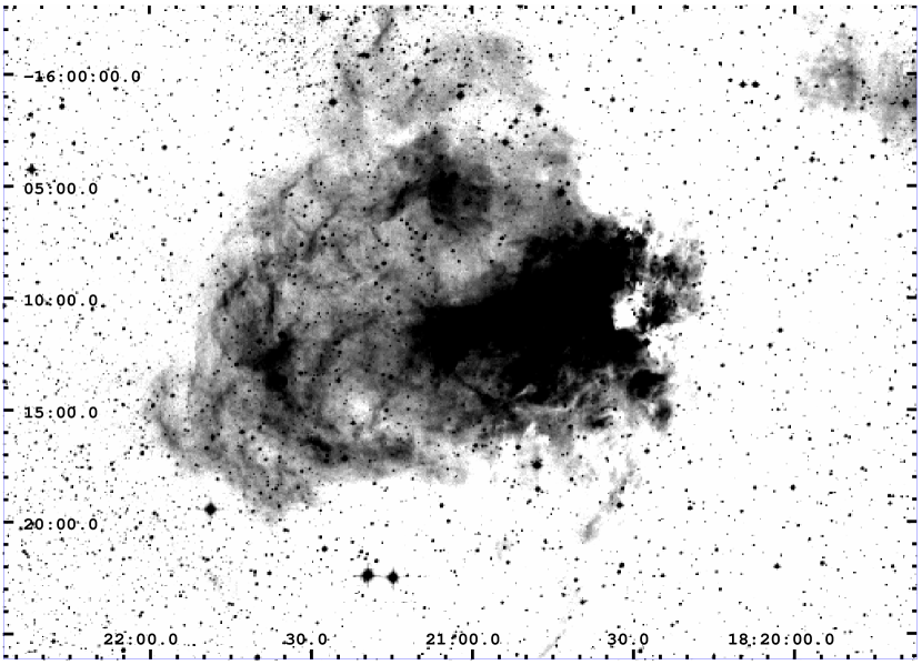
Figure 1: Image of the omega nebulae from the Digital Sky Survey (DSS). It is illuminated by the massive stellar cluster NGC 6618, the centre of which is located behind substantial obscuring material, with $A_{\nu}\sim 8$ mag.

The centre of the stellar cluster NGC 6618 consists of a ‘ring’ of seven O-type stars (Hanson et al. 1997) which are located between the two bars. These stars must be the dominant sources of ionising photons on the nebula, in fact diffuse X-ray emission is observed to be well confined within the external shell of the optical nebula (Dunne et al. 2003). Figure 1 shown a DSS image of this object. The ring of seven O-type stars is located on the West, where is substantial obscuring material, with $A_{\nu}\sim 8$ mag (Hanson et al. 1997).

The stellar winds of these seven stars strongly contribute to the formation of a common ‘stellar cluster wind’ (Cantó et al., 2000). The collision of these winds with the surrounding inhomogeneous ISM produces the diffuse X-ray emission observed by ROSAT and Chandra satellites.

In ROSAT images, M17 is observed as a blister-like structure, with an overall diameter of $\sim 10-12~{}\mathrm{pc}$, if a distance of $1.6~{}\mathrm{kpc}$ is considered (Nielbock et al. 2001). The emission peak is located inside the stellar cluster. This suggested that the cluster is the origin of the diffuse X-ray emission, and was later confirmed by Chandra observations (Townsley et al. 2003), where the angular resolution allowed to see the individual sources. M17 was observed with ROSAT Position Sensitive Proportional counter (PSPC) for $6.7$ ks in the $0.1-2.4$ keV band (Dunne et al. 2003). They found a total diffuse X-ray luminosity of $\sim 2.5\times 10^{33}\mathrm{erg~{}s^{-1}}$ with kT = 0.66-0.78 keV ($T=7.7-9.1\times 10^{6}$ K) and $N_{H}=(1-5)\times 10^{21}~{}\mathrm{cm^{-2}}$.

Several models have tried to reproduce the total X-ray luminosity $\mathrm{L_{X}}$ from superbubbles, often taking into account the effects of the electron thermal conduction. However, the $\mathrm{L_{X}}$ reproduced by models where thermal conduction is included (Weaver et al. 1977) is usually two or three orders of magnitude higher than the observed values, while models where thermal conduction is ignored predict a $\mathrm{L_{X}}$ that is typically two orders of magnitude lower than observed. Most of the time the descriptions are rather simple, they consider for instance that the cluster wind interacts with an homogeneous and isotropic ISM, and neglect the effects of radiative cooling. For M17 this approach is not adequate because it is a star forming region surrounded by asymmetrically distributed high density molecular clouds.

In this work we present three-dimensional numerical simulations based on the properties of M17. The simulations were carried out with the adaptive grid code yguazú-a, and considered the main characteristics of the ISM that surrounds M17. Synthetic thermal X-ray emission maps were obtained from the numerical results in order to compare the morphology and the total luminosity directly with ROSAT X-ray observations (with a field of view of $\sim 2\degr$).

This manuscript is organised in the following way: in section 2 we explain the modelling of M17, the initial conditions of numerical simulations, and describes the simulation of the thermal X-ray emission; an archival ROSAT image of this superbubble is presented in section 3; the results and comparison with observations are given in section 4; and finally in section 5 we summarise our conclusions.

Table 1: OB Stars in M17 and their stellar wind parameters.

Name	R.A.(J2000.0)	DEC.(J2000.0)	Optical	K-Band	$V_{\infty}$	$\dot{M}$
	($\aas@@fstack{h}$ $\aas@@fstack{m}$ $\aas@@fstack{s}$)	(° ′ ″)	Spectral type	Spectral type	( $\mathrm{km~{}s^{-1}}$ )	($\mathrm{M_{\odot}~{}yr^{-1}}$ )	References
B98	18 20 35.45	$-$16 10 48.9	O9 V	kO9-B1	2200	$2.6\times 10^{-7}$	1,2,3
B111	18 20 34.55	$-$16 10 12.1	O5 V	kO3-O4	3250	$1.86\times 10^{-6}$	3
B137	18 20 33.14	$-$16 11 21.6		kO3$-$O4	3370	$2.4\times 10^{-6}$	4,5
B164	18 20 30.92	$-$16 10 08.0	O7$-$O8 V	kO7-O8	3015	$2\times 10^{-6}$	1,4
B174	18 20 30.54	$-$16 10 53.3		k03$-$O6	3370	$6.5\times 10^{-7}$	1,4
B181	18 20 30.30	$-$16 10 35.2		kO9$-$B2	2200	$2.6\times 10^{-7}$	1,2,3
B189	18 20 29.92	$-$16 10 45.5	O5 V	kO3$-$O4	3250	$1.86\times 10^{-7}$	3
B260	18 20 25.94	$-$16 08 32.3	O7$-$O8 V	kO3-O4	3015	$2\times 10^{-6}$	1,4
B289	18 20 24.45	$-$16 08 43.3	O9.5 V		1500	$2.5\times 10^{-7}$	1,6
B311	18 20 22.76	$-$16 08 34.3		kO9$-$B2	2200	$2.6\times 10^{-7}$	1,2,3
OI 345	18 20 27.52	$-$16 13 31.8	O6 V	kO5-O6	3065	$6.5\times 10^{-7}$	1,4

References.–(1) de Jager et al. 1988; (2) Wilson & Dopita 1985; (3) Leitherer 1988; (4) Prinja et al. 1990; (5) Lamers & Leitherer 1993; (6) Fullerton et al. 2006

2 Modelling the M17 nebula

As it was mentioned above, the stars that belong to the NGC 6618 cluster are too young to generate SN explosions. For this reason, the M17 nebula was modelled by the interaction of stellar winds alone. We only considered the stars that dominate the mechanical luminosity of the cluster, they have high terminal velocities and mass loss rates, the values are based on the spectral types reported by Hanson et al. (1997), we list them in Table LABEL:tabstar. The values for the terminal velocity and mass loss rate correspond to the upper limits reported in the literature (de Jager et al. 1988; Wilson & Dopita 1985; Leitherer 1988; Prinja et al. 1990; Lamers & Leitherer 1993; Fullerton et al. 2006). This has been done with the intention to increase the X-ray luminosities obtained from our simulations, and to compensate for the fact that all the other wind sources have been disregarded. Furthermore, a recent study of Hoffmeister et al. (2008) has shown that the number of stars in the NGC 6618 cluster is even higher than previous estimates.

For the 3D numerical simulations we consider that the plane of the sky corresponds to the $xy-$plane of our simulation. Table LABEL:tabstar gives the position of the stars in equatorial coordinates (J2000), which can be translated to parsecs considering that the cluster is at a distance of $1.6~{}$kpc.

Since we do not know the individual line-of-sight distance ($z-$coordinate) to the stars, we produced three different realisations of randomly picked positions in $z$, while keeping the same $xy$ configuration (see Figure 2). The maximum of the distribution from which the $z$ positions were sampled was set to the maximum separation in the plane of the sky, and the mean was set to the distance to the cluster ($1.6~{}\mathrm{kpc}$.) The resulting $yz$ distributions are shown in Figure 3.

The NGC 6618 cluster is bounded by two molecular clouds at the North and South-West, observed in HI (Felli et al. 1984). These clouds have the appearance of a wedge which confine the resulting stellar cluster wind, and produce an elongated structure to the East. We model the clouds as two bars one of them is horizontal (we will reefer to it as the ‘top bar’) and the other one tilted 45°in the $xy$-plane (which we will call the ‘bottom bar’). Their surfaces are flat, and cover the entire extent of the computational domain along the $z$ axis (i.e. the geometry displayed in Figure 2 is the same for all values of $z$). The bars have a high density contrast with respect to the surrounding ISM (of two orders of magnitude). The stars (wind-sources) were placed inside the wedge formed by the two bars, as shown schematically in Figure 2.

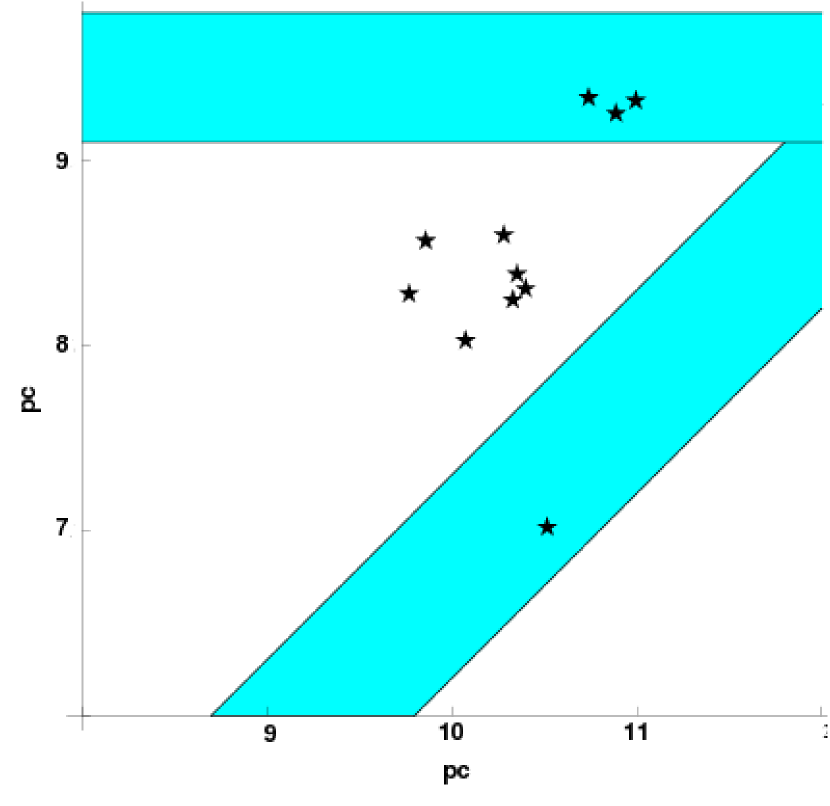
Figure 2: Stellar positions in the plane sky (the $xy-$ plane). These positions were calculated considering the R.A and Dec. positions listed on Table LABEL:tabstar and a cluster distance of 1.6kpc. The shaded area represents the location of the dense molecular clouds that surround the M NGC 6618 cluster.

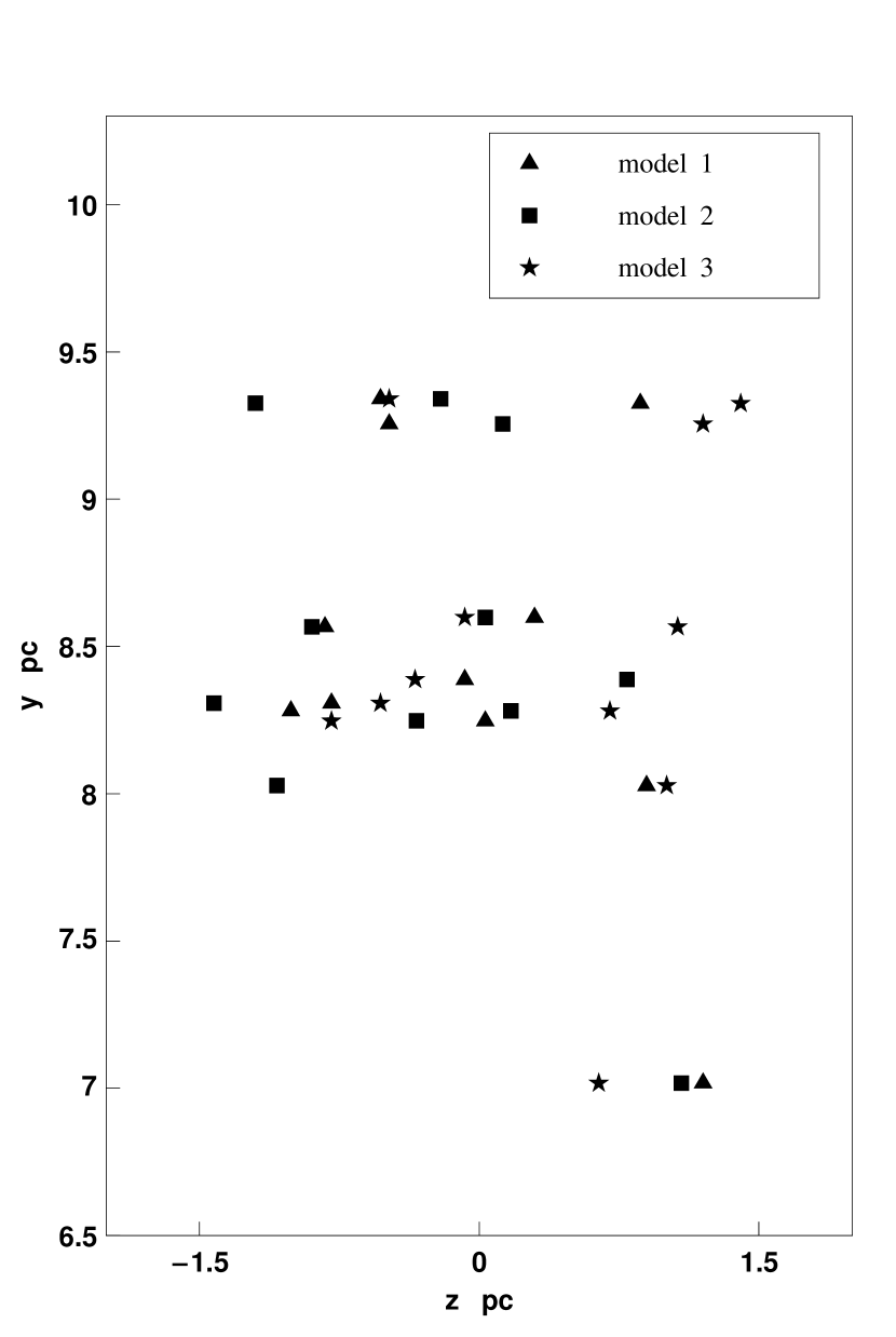
Figure 3: Stellar configuration in the $yz-$plane for each of the models, as indicated in the legend.

2.1 Initial setup

We have carried out the 3D numerical simulations with the yguazú-a hydrodynamical code (Raga et al., 2000, 2002). The code integrates the gasdynamic equations with a second-order accurate implementation of the flux vector splitting method of van Leer (1982) on a binary adaptive grid. This code was first tested comparing simulations of shock waves and laser laboratory experiments (one bubble shock wave, Raga et al. 2000; two interacting bubbles, Velázquez et al. 2001). In last 8 years, the yguazú-a code has been widely used to model several different astrophysical scenarios, such as Herbig Haro objects (Raga et al., 2002; Masciadri et al., 2002), supernovae remnants (Schneiter et al., 2006; Reyes-Iturbide et al., 2008), jets in planetary nebulae (Velázquez et al., 2004; Guerrero et al., 2008), interacting winds (González et al., 2004; Rodríguez-González et al., 2007), and exoplanets (Schneiter et al., 2007).

For this problem we use a computational domain with a physical size of ($12\times 12\times 4$) pc ($x-$,$y-$, and $z-$axis, respectively), and allow five levels of refinement, such that the resolution at the finest level of is $7.27\times 10^{16}$ cm. This would correspond to $512\times 512\times 128$ pixels in a uniform grid. We chose this spatial resolution ($3\arcsec$ if a distance of $.1.6~{}\mathrm{kpc}$ to M17 is assumed) to match the resolution of ROSAT raw observations ($\sim 4\arcsec$, see §3.)

The stellar winds are imposed in spheres (centred at the stellar positions) of radius $R_{w}=4.4\times 10^{17}$ cm, which corresponds to 6 pixels at the maximum resolution of the adaptive grid (always present at the wind sources). Within these spheres, we inject at every time-step material at $T_{w}=1000$ K, with the outward velocity given in Table LABEL:tabstar for each star. The density inside the spheres follows an $r^{-2}$ law (where $r$ is the radial coordinate measured outwards from the stellar position), scaled to yield the mass loss rates in Table LABEL:tabstar.

The stars and the bars are located in the top-right quadrant of the numerical domain, in the $xy-$ plane. The bars were initialised with a uniform number density of 1000 cm^-3 and a temperature of 400 K in order to stay in pressure equilibrium with an ISM that has a density of 10 cm^-3, and a temperature of 10⁴ K.

2.2 Simulated X-ray emission

The numerical simulation provides us with density and temperature distributions for each model, which we combine with synthetic X-ray spectra to simulate the X-ray emission of M17.

The synthetic spectra were obtained with the chianti database (Dere et al., 1997; Landi et al., 2006). We calculate the X-ray emission coefficient $j_{\nu}(n,T)$ in the energy range of 0.1-2.4 keV to coincide with that of ROSAT. Based on observational works (Dunne et al., 2003; Townsley et al., 2003; García-Rojas et al., 2007) a solar abundance was assumed for M17, together with the ionisation equilibrium model of Mazzotta et al. (1998). The $j_{\nu}(n,T)$ coefficients are calculated in the limit of low density regime, which results in $j_{\nu}(n,T)\propto n^{2}$. To produce X-ray maps the absorption is included, assuming a uniform hydrogen column density of $N_{H}=3.2\times 10^{21}\ \mathrm{cm}^{-2}$.

3 ROSAT image of M17

M17 was observed with the ROSAT satellite, with the Position Sensitive Proportional Counter (PSPC) detector. This instrument is sensitive to X-ray photons with energies in the range $0.1-2.4$ keV and has an spectral resolution energy of $\sim 40\%$ at 1 keV, with a field of view of $\sim 2^{o}$, covering the entire dimensions of superbubble M17 (with an angular size of $\sim 23\arcmin\times 20\arcmin$).

We have used an image (binned to $4\arcsec$ per pixel) from archival ROSAT Catalogue of PSPC WGA sources, which corresponds to the PSPC observations of M17 (id:WP500311) obtained on September 12-13, 1993, with an exposure time of $6.7$ ks. In order to study the spatial distribution of the X-ray emission from M17, we have increased the signal to noise ratio using the standard procedure of smoothing the image (Dunne et al. 2003, Townsley et al. 2003). To do this, we convolved the observations with a Gaussian function with an effective PSF of $5.4$ pixels. In Figure 5 we show the original (raw data) image and the smoothed version.

4 Results and discussion

We ran the models up to an integration time of $1.3\times 10^{5}$ yr, which is the estimated superbubble age (Weaver et al. 1977). In Figure 4 we present X-ray emission maps for the three models at their latest integration time. These maps show the absorbed X-ray emission, assuming a column density of $3.2\times 10^{21}\ \mathrm{cm}^{-2}$ as found from ROSAT observations (Dunne et al. 2003).

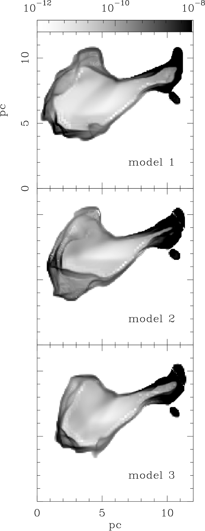
Figure 4: Simulated X-ray emission maps obtained from models 1, 2, and 3 (from the top to the bottom) in the energy range $0.1-2.4$ keV, an absorption due to $N_{H}=3.2\times 10^{21}\mathrm{cm^{-2}}$ has been included. Maps corresponding to models 1 and 2 show more evolved superbubbles (produced by the cluster wind). The bar on the top gives the logarithmic grey-scale in units of erg cm^-2 s^-1 sr^-1. The vertical and horizontal axis are given in units of pc.

The interaction of many individual stellar winds will coalesce into a common cluster wind, as studied for massive stellar clusters by Cantó et al. (2000) and Rodríguez-González et al. (2007). However, unlike those models that consider a uniform ISM, we can see from Figure 4 that the resulting X-ray emission is not homogeneous. All models show a strong concentration of X-ray emission in regions to the top right of each map, especially for model 2. This enhancement corresponds to strong shock waves produced by the collision of the cluster wind with the dense molecular cloud or bars. These bars are flat and focus the cluster wind flow and produce the elongated morphology observed in X-rays. To the opposite side the cluster wind can expand more freely producing through a ‘champagne’-type flow a superbubble of $\sim 12~{}\mathrm{pc}$ in size. From Figure 4, the structure seen in our simulations at the position $x\sim 10\mathrm{pc}$, $y\sim 7\mathrm{pc}$ corresponds to the wind of an isolated star embedded in the the southern bar, which gets confined due to the high density of its surrounding medium (see Fig. 2).

The surrounding dense bars have another important effect, namely to increase the total X-ray luminosity $\mathrm{L_{X}}$. This effect depend on the geometry of the bars, which in our models we have considered to be flat (independent of $z$). If they would have a concave section, the cluster wind would be more strongly focused, increasing the $\mathrm{L_{X}}$, and the opposite would be true if they were convex. To analyse influence of the bars, we have run an additional model (not presented here), removing them from the numerical setup. In that case the cluster wind is free to sweep the less dense ISM, and results in a $\mathrm{L_{X}}$ 2 orders of magnitude lower than the obtained one from Models 1, 2, and 3. This shows the importance of considering the characteristics of the environment of M17, in particular the dense molecular cloud that surrounds the open cluster NGC 6618.

In Table LABEL:tablum we list the $\mathrm{L_{X}}$ obtained for all the models. We must notice that the X-ray luminosity listed there has been calculated directly from the X-ray emission coefficients derived from the simulations, thus no correction for absorption is needed. In other words, it should be compared with the X-ray luminosity of observations after these observations have been corrected for absorption. Models 1, 2, and 3 produce similar luminosities, all of them on the order of 60 per cent of the observed value (although Model 1 gives a slightly lower value). One has to bear in mind that the gas in the bar is not uniform in reality, but it has high density clumps (Townsley et al. 2003). The inclusion of such clumps could somewhat increase the total X-ray luminosity compared with that obtained in our models.

Other factor that can change the obtained $\mathrm{L_{X}}$ is the metal abundance. To estimate importance of this factor, we generated new X-ray coefficients (with the CHIANTI atomic database) considering different values of the metalicity $Z$ around of the solar value. The resulting luminosities are listed in table LABEL:tablum2. For $Z=0.3$, the X-ray luminosity is 2.7 times lower than the obtained for $Z=1$ (solar abundance). We must note, however, that this is only a rough estimate. A detailed study of the effect of metalicity on the X-ray luminosity would have to include the dynamical effect that results from a modified radiative cooling. In any case, recent work (García-Rojas et al., 2007) show that abundances close to the solar ones are adequate for M17.

Dunne et al. (2003) obtained a total X-ray luminosity of $5\times 10^{35}\mathrm{erg\ s^{-1}}$ for M17, employing both the Weaver et al. (1977) bubble model, and the Chu et al. (1995) superbubble model. Such value is two orders of magnitude higher than the observed one. These models are based on the evolution of bubbles (and superbubbles) into an homogeneous medium, and they are adiabatic, although they include thermal conduction effects. In our case, it was not necessary to include the last physical process because we have obtained a $\mathrm{L_{X}}$ already compatible with observations, taking only into account the inhomogeneity of surrounding ISM, and including the radiative cooling.

Although thermal conduction effects should be present, as firstly introduced in the wind-blown bubble model by Weaver et al. (1977), there are important discrepancies between the X-ray luminosities predicted by that model and what is observed. For instance, X-ray emission should be detected in almost all the known wind-blown bubbles and superbubbles, but this is not the case (see Mac Low 2000, for a discussion). In particular, for M17, a direct application of Weaver’s et al. model (which considers thermal conduction as a crucial ingredient for the X-ray emission of the hot interior) predicts an X-ray luminosity about 100 times higher than what is measured (Dunne et al. 2003). This leads us to think that perhaps some mechanisms are present that inhibit thermal conduction, at least in the form that it is treated in Weaver’s et al. model. The presence of magnetic fields is often invoked as one of the possible inhibiting factors. In our particular case, we show that whatever mechanism might be at work, thermal conduction do not seem to play an important role in the prediction of X-ray emission from the M17 superbubble.

Table 2: Total X-ray luminosities.

	$\mathrm{L_{X}}$ ($10^{33}~{}\mathrm{erg~{}s^{-1}}$)
ROSAT observation	$2.5$
Model 1	$1.4$
Model 2	$1.6$
Model 3	$1.6$

Table 3: Metalicity vs Total X-ray luminosities.

$Z$	$\mathrm{L_{X}}$ ($10^{33}~{}\mathrm{erg~{}s^{-1}}$)
0.3	0.6
0.5	0.9
0.7	1.2
0.9	1.4
1.0	1.6
1.1	1.7
1.3	2.0

The X-ray emission distribution for all models (see Figure 4) show a general gradient, with lower emission to the left, in coincidence with the observations (see Figure 5). Also in our models, on the left of the X-ray emitting material, strong emission is observed in form of filaments (see Figure 4). These filaments trace the shock front of champagne flow described above, propagating into the surrounding ISM. In ROSAT observations, bright regions or ‘clumps’ can be seen to the East (corresponding to the left, in our simulations). These clumps can be produced by the propagation of strong shock waves into an inhomogeneous medium. However, these features are smoother than those obtained from the simulations probably due to the difference between observed and simulated resolutions. To make a fair comparison we show in Figure 6 a smoothed synthetic map of model 2, produced by convolving the numerical results with a Gaussian beam in order to reproduce the same resolution of the ROSAT (smoothed) image in Fig. 5.

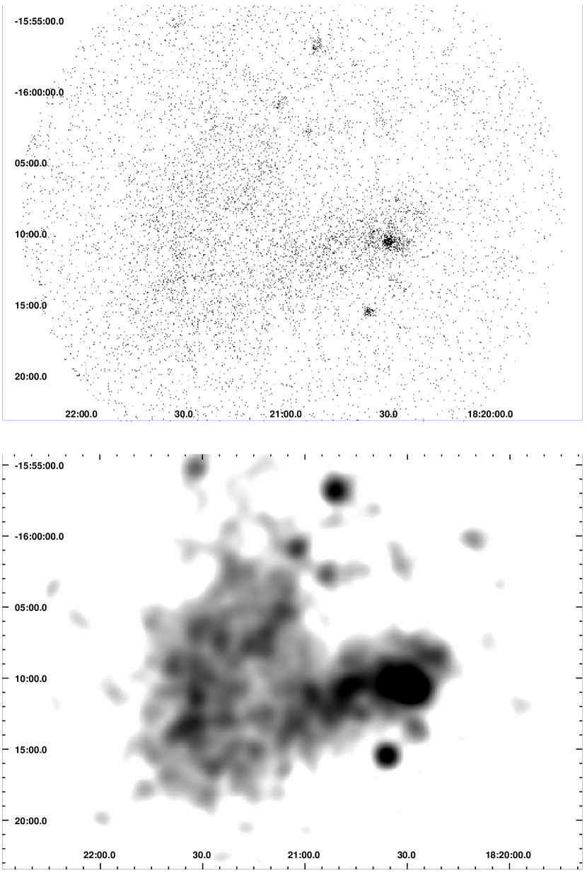
Figure 5: ROSAT image of superbubble M17, obtained from archival data (ROSAT catalogue of PSPC WGA sources) in the energy range $0.1-2.4$ keV. Top panel: raw data binned to $4\arcsec$ per pixel. Bottom panel: Smoothed image obtained after convolving with a Gaussian function with a PSF of $5.4$ pixels.

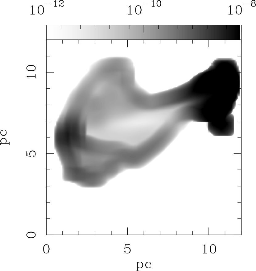
Figure 6: Synthetic X-ray emission map of model 2 in the energy range $0.1-2.4$ keV, smoothed with the same resolution of the ROSAT observation (Figure 5). The bar on the top is the logarithmic grey-scale, which is given in units of erg cm^-2 s^-1 sr^-1. Vertical and horizontal axis are given in units of pc.

5 Conclusions

We carried out 3D numerical simulations using the adaptive grid code yguazú-a to model the M17 superbubble. Radiative losses have been included in the simulations. Three different runs of the same model were made using the known positions of the dominant wind sources on the plane of the sky (corresponding to the $xy$ positions in our Cartesian grid), and considering three different distributions along the line of sight (aligned with our $z-$axis).

Our results show that the inclusion of the main features of the surrounding ISM (i.e. the presence of two dense bars or clouds around the M17 stars) plays a crucial role to explain both the observed morphology and the total X-ray luminosity of this object.

On the one hand, the bars produces in all models a ‘champagne’ flow effect, in which the resulting stellar cluster wind is focused by such bars, producing an elongated shape in the $x-$ direction, thus reproducing the elongated shape in the East-West direction of the observations.

On the other hand, the collision of the cluster wind with the bars maintains a high-temperature, high-density distribution in the region between the bars. This is a product of the multiple reflected shocks, and enhances the total X-ray luminosity ($\mathrm{L_{X}}$). We obtain values of the total X-ray luminosity of $\simeq 1.6\times 10^{33}\mathrm{erg\ s^{-1}}$, which are in agreement with observations.

The different $z-$ stellar distributions employed in our runs had a rather small effect on both the morphology and $\mathrm{L_{X}}$. This could be somewhat expected, because the same mechanical luminosity input is used for all the runs, and because away of the cluster centre the common wind that forms should be similar. Finally, it is noticeable that we obtain a reasonable estimate of the total X-ray luminosity without the need of including thermal conduction effects.

References

- Brogan & Troland (2001) Brogan, C. L., & Troland, T. H. 2001, ApJ, 560, 821
- Broos et al. (2007) Broos, P. S., Feigelson, E. D., Townsley, L. K., Getman, K. V., Wang, J. F., Garmire, G. P., Jiang, Z., & Tsuboi, Y. 2007, ApJS, 169, 353
- de Jager et al. (1988) de Jager, C., Nieuwenhuijzen, H., & van der Hucht, K. A. 1988, A&AS, 72, 259
- Cantó et al. (2000) Cantó, J., Raga, A. C., & Rodríguez, L. F. 2000, ApJ, 536, 896
- Chu et al. (1995) Chu, Y.-H., Chang, H.-W., Su, Y.-L., & Mac Low, M.-M. 1995, ApJ, 450, 157
- Dere et al. (1997) Dere, K. P., Landi, E., Mason, H. E., Monsignori Fossi, B. C., & Young, P. R. 1997, A& AS, 125, 149
- Dunne et al. (2003) Dunne, B. C., Chu, Y.-H., Chen, C.-H. R., Lowry, J. D., Townsley, L., Gruendl, R. A., Guerrero, M. A., & Rosado, M. 2003, ApJ, 590, 306
- Felli et al. (1984) Felli, M., Churchwell, E., & Massi, M. 1984, A& A, 136, 53
- Fullerton et al (2006) Fullerton, A. W., Massa, D. L., & Prinja, R. K. 2006, ApJ, 637, 1025
- García-Rojas et al. (2007) García-Rojas, J., Esteban, C., Peimbert, A., Rodríguez, M., Peimbert, M., & Ruiz, M. T. 2007, Revista Mexicana de Astronomia y Astrofisica, 43, 3
- González et al. (2004) González, R. F., de Gouveia Dal Pino, E. M., Raga, A. C., & Velázquez, P. F. 2004, ApJ, 616, 976
- Guerrero et al. (2008) Guerrero, M. A., et al. 2008, ApJ, 683, 272
- Hanson et al. (1997) Hanson, M. M., Howarth, I. D., & Conti, P. S. 1997, ApJ, 489, 698
- Hoffmeister et al. (2008) Hoffmeister, V. H., Chini, R., Scheyda, C. M., Schulze, D., Watermann, R., Nürnberger, D., & Vogt, N. 2008, ApJ, 686, 310
- Knödlseder et al. (2002) Knödlseder, J., Cerviño, M., Le Duigou, J.-M., Meynet, G., Schaerer, D., & von Ballmoos, P. 2002, A& A, 390, 945
- Lada et al. (1974) Lada, C., Dickinson, D.F., & Penfield, H. 1974, ApJ, 189, L35
- Lada et al. (1991) Lada, C. J., Depoy, D. L., Merrill, K. M., & Gatley, I. 1991, ApJ, 374, 533
- Landi et al. (2006) Landi, E., Del Zanna, G., Young, P. R., Dere, K. P., Mason, H. E., & Landini, M. 2006, ApJS, 162, 261
- Lamer & Leitherer (1993) Lamers, H. J. G. L. M., & Leitherer, C. 1993, ApJ, 412, 771
- Leitherer (1988) Leitherer, C. 1988, ApJ, 326, 356
- Masciadri et al. (2002) Masciadri, E., Velázquez, P. F., Raga, A. C., Cantó, J., & Noriega-Crespo, A. 2002, ApJ, 573, 260
- McCray & Kafatos (1987) McCray, R., & Kafatos, M. C. 1987, ApJ, 317, 190
- Mac Low & McCray (1988) Mac Low, M.-M., & McCray, R. 1988, ApJ, 324, 776
- Mac Low (2000) Mac Low, M.-M. 2000, Revista Mexicana de Astronomia y Astrofisica Conference Series, 9, 273
- Mazzotta et al. (1998) Mazzotta, P., Mazzitelli, G., Colafrancesco, S., & Vittorio, N. 1998, A& AS, 133, 403
- Nielbock et al. (2001) Nielbock, M., Chini, R., Jütte, M., & Manthey, E. 2001, A& A, 377, 273.
- Prinja et al. (1990) Prinja, R. K., Barlow, M. J., & Howarth, I. D. 1990, ApJ, 361, 607
- Raga et al. (2000) Raga, A. C., Navarro-González, R., & Villagrán-Muniz, M. 2000, Revista Mexicana de Astronomia y Astrofisica, 36, 67
- Raga et al. (2002) Raga, A. C., de Gouveia Dal Pino, E. M., Noriega-Crespo, A., Mininni, P. D., & Velázquez, P. F. 2002, A& A, 392, 267
- Reyes-Iturbide et al. (2008) Reyes-Iturbide, J., Rosado, M., & Velázquez, P. F. 2008, AJ, 136, 2011
- Rodríguez-González et al. (2007) Rodríguez-González, A., Cantó, J., Esquivel, A., Raga, A. C., & Velázquez, P. F. 2007, MNRAS, 380, 1198
- Schneiter et al. (2006) Schneiter, E. M., de La Fuente, E., & Velázquez, P. F. 2006, MNRAS, 371, 369
- Schneiter et al. (2007) Schneiter, E. M., Velázquez, P. F., Esquivel, A., Raga, A. C., & Blanco-Cano, X. 2007, ApJL, 671, L57
- Townsley et al. (2003) Townsley, L.K., Feigelson, E., Montmerle, T., Broos, P., Chu, Y., Garmire, G.P. 2003, ApJ, 593, 874
- van Leer (1982) van Leer, B. 1982, Numerical Methods in Fluid Dynamics, 170, 507
- Velázquez et al. (2001) Velázquez, P. F., Sobral, H., Raga, A. C., Villagrán-Muniz, M., & Navarro-González, R. 2001, Revista Mexicana de Astronomia y Astrofisica, 37, 87
- Velázquez et al. (2004) Velázquez, P. F., Riera, A., & Raga, A. C. 2004, A& A, 419, 991
- Weaver et al. (1977) Weaver, R., McCray, R., Castor, J., Shapiro, P. & Moore, R., 1977, ApJ, 218, 377.
- Wilson & Dopita (1985) Wilson, I. R. G., & Dopita, M. A. 1985, A&A, 149, 295