Cooperative Multiplexing in the Multiple Antenna Half Duplex Relay Channel

Abstract

Cooperation between terminals has been proposed to improve the reliability and throughput of wireless communication. While recent work has shown that relay cooperation provides increased diversity, increased multiplexing gain over that offered by direct link has largely been unexplored. In this work we show that cooperative multiplexing gain can be achieved by using a half duplex relay. We capture relative distances between terminals in the high SNR diversity multiplexing tradeoff (DMT) framework. The DMT performance is then characterized for a network having a single antenna half-duplex relay between a single-antenna source and two-antenna destination. Our results show that the achievable multiplexing gain using cooperation can be greater than that of the direct link and is a function of the relative distance between source and relay compared to the destination. Moreover, for multiplexing gains less than 1, a simple scheme of the relay listening 1/3 of the time and transmitting 2/3 of the time can achieve the 2 by 2 MIMO DMT.

I Introduction

There is a growing interest in the design of cooperative schemes that provide diversity and multiplexing gain for communication via wireless relays. Cooperative diversity refers to the additional diversity gain (compared to direct link) offered by cooperation. Similarly if a relay provides additional degrees of freedom (compared to direct link) it is said to provide a cooperative multiplexing gain [1].

Diversity multiplexing tradeoff (DMT) [2] has been widely used to analyze and compare the performance of cooperative schemes. DMT for the half-duplex single relay network has been studied extensively in literature [3][4][5]. For the case with single antennas at all terminals the $2\times 1$ MISO DMT bound has recently been shown [5] to be achievable. In this paper we study the DMT for the multiple antenna half-duplex relay channel having $m,n$ and $k$ antennas at source, destination and relay respectively. This was studied in [4] but results were shown only for the special case $m=n=1$. We calculate the maximum achievable DMT for the $m=1,n=2,k=1$ configuration. In the process we also demonstrate techniques that enable results for general $m,n$ and $k$. $m=1,n=2,k=1$ is the simplest configuration where relay cooperation provides additional multiplexing gain compared to direct link. We show that if source and relay are relatively close to each other, cooperative multiplexing gain is achievable even with half duplex relaying. Note that the full-duplex case has been studied in [1]. Moreover, for multiplexing gains less than $1$, if source-relay SNR (measured in dB) is at least two times the source-destination SNR a simple scheme with the relay listening $\frac{1}{3}$ of the time and transmitting $\frac{2}{3}$ of the time can achieve the $2\times 2$ MIMO DMT.

These results lend fresh insight into the fundamental limits of cooperative multiplexing in the half-duplex relay channel. We demonstrate the use of two key techniques that enable our results.

1. Distance between terminals: In most results it is seen that relative distances between source, relay and destination do not affect DMT performance of the relay channel. Since DMT is calculated at high SNR the path loss and therefore distances are not easily captured in results. We overcome this apparent limitation by scaling the average SNR’s of the various links differently.

   Our approach enriches the DMT framework by adding insights about network geometry.

2. MIMO with half duplex antenna: The min-cut capacity bound has been used in [4] to calculate an upper bound for DMT performance. Notice in Figure 1 that the $\{S,R\},\{D\}$ cut corresponds to a $2\times 2$ MIMO system with one source antenna that remains active only for a fraction of total communication time ($R$ is half duplex). It was noted [4] that an upper bound for mutual information across such a cut is hard to compute. Due to this, DMT bounds have only been reported for the special case of $m=n=1$.

   In Sec III-A we demonstrate a simple channel decomposition that allows us to compute the cut-set DMT bound for the $m=1,n=2,k=1$ configuration. The technique can be applied towards computing DMT bounds for general $m,n$ and $k$. Recent results in [7] [8] show that a simple relaying scheme called “quantize-map” can achieve a rate within constant gap of the cut-set capacity. In Sec IV we discuss this scheme and show that it achieves the cut-set DMT bound.

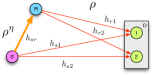
Figure 1: Relay channel with $2$ antennas at destination and $S\to R$ proximity gain $\eta$.

II System Model

Consider the system in Figure 1 with source $S$, relay $R$ and destination $D$ having $1,1$ and $2$ antennas respectively. Let $D_{j},j\in\{1,2\}$ denote the $j$th antenna at $D$. The channel gain for $S\to R$ is $h_{sr}$, gains for $S\to D_{j}$ are $h_{sj}$ and $R\to D_{j}$ are $h_{dj}$. All the channel gains are assumed to be flat fading having i.i.d. $\mathcal{CN}(0,1)$ distribution. We assume quasi-static fading, i.e. once realized, channel gains remain unchanged for the duration of the codeword and change independently between codewords. Noise at all receivers is additive i.i.d. $\mathcal{CN}(0,1)$ and independent of all other variables in the system. Transmit power at $S$ and $R$ is limited by an average power constraint. Since noise power at receiver is normalized to $1$, the transmit power constraint is specified by the average Signal to Noise Ratio (SNR). $R$ is assumed to operate under a half-duplex constraint. For simplicity it is assumed that transmissions at $S$ and $R$ are synchronous at symbol level.

We assume an asymmetrical network geometry. $S$ and $R$ are modeled to be close to each other as compared to $\{S,R\}$ and $D$. $S\to D$ and $R\to D$ are assumed to have the same average SNR denoted by $\rho$. $S\to R$ on the other hand is modeled to have SNR higher than $\rho$ by a factor $\eta$ on dB scale, i.e. the $S\to R$ average SNR is $\rho^{\eta}$. The $S\to R$ channel (cooperation link) thus has $\eta-1$ more degrees of freedom than other channels in the network. We call $\eta$ the proximity gain and assume $\eta\geq 1$.

No channel state information (CSI) is available at $S$ i.e. only average channel statistics $\rho,\eta$ are known. However, at $D$ all channel realizations $h_{sr}$, $h_{sj},h_{dj}$ are completely known.

We identify three models for relaying strategy.

• Global: The relay uses knowledge of all instantaneous channel realizations to optimize its strategy.

• Local: The relay can measure $h_{sr}$ and uses only this (local) information.

• Blind: The relay only uses average channel statistics.

The global strategy is discussed in Sec III while local and blind are discussed in Sec V.

III Diversity-Multiplexing Tradeoff

Figure 2: $d(r)$ for various values of proximity gain $\eta$.

Theorem III.1

The maximum achievable DMT for network described in Sec II is given by,

$$d(r)=\left\{\begin{array}[]{cc}\min\{\eta+2,4\}-3r&0\leq r\leq 1,\eta\geq 1\\ (2\eta-\eta r-1)/(\eta-r)&1\leq r\leq 2-\frac{1}{\eta},\eta\geq 2\\ \eta-\frac{1}{2-r}&1\leq r\leq 2-\frac{1}{\eta},1\leq\eta\leq 2\end{array}\right.$$ (1)

Corollary III.2

For system model described in Sec II the maximum achievable multiplexing gain $r^{*}=\inf_{r\geq 0}\{r|d(r)=0\}$ is,

$$r^{*}=2-\frac{1}{\eta}$$ (2)

For a symmetrical geometry with all channels having the same degrees of freedom ($\eta=1$) we get $r^{*}=1$ i.e. cooperation doesn’t provide additional maximum multiplexing gain. To enable higher multiplexing gain the $S\to R$ channel (cooperation link) needs to have more degrees of freedom than the $S\to D$ channel (communication link).

Let $d_{2\times 2}(r)$ represent the DMT of the $2\times 2$ MIMO channel. For finite $\eta$ it can be seen that $d(r)\leq d_{2\times 2}(r)$ with strict inequality over a non-empty region of $r$. This suggests that for distributed antennas the finite capacity of the cooperation channel $(S\to R)$ poses a fundamental limitation on the achievable DMT performance. It can easily be verified that,

$$\lim_{\eta\to\infty}d(r)\to d_{2\times 2}(r)$$

Figure 2 shows $d(r)$ for several values of $\eta$.

We prove Theorem III.1 in two steps. In Sec III-A we show that the cut-set DMT upper bound for network in Sec II is given by (1). In Sec IV we show that this bound is achievable.

III-A Cut-Set DMT upper bound

Let $f(0\leq f\leq 1)$ denote a listen-transmit schedule for the half duplex relay. $R$ listens for a fraction $f$ (listening phase) of total communication time and transmits for fraction $(1-f)$ (cooperation phase). The two cuts of the network $\mathcal{C}_{D}=\{S,R\},\{D\}$ and $\mathcal{C}_{S}=\{S\}\{R,D\}$ are shown in Figure 3 for these two phases. In the listening phase let $\mathbf{X}_{S}^{1}$ denote the sequence of symbols transmitted by $S$ while $\mathbf{Y}_{R}$ and $\mathbf{Y}_{D}^{1}$ denote received signals at $R$ and $D$ respectively. Similarly for the cooperation phase $\mathbf{X}_{S}^{2}$ and $\mathbf{X}_{R}$ are the symbol sequences transmitted from $S$ and $R$ while $\mathbf{Y}_{D}^{2}$ is received at $D$. The instantaneous mutual information across the two cuts can be written as,

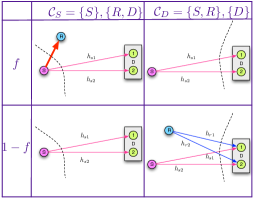
Figure 3: Two cuts of network during listen $(f)$ and cooperation phase.$(1-f)$.

$$I_{\mathcal{C}_{S}} = fI(\mathbf{X}_{S}^{1};\mathbf{Y}_{R},\mathbf{Y}_{D}^{1}|\mathbf{X}_{R})+(1-f)I(\mathbf{X}_{S}^{2};\mathbf{Y}_{D}^{2}|\mathbf{X}_{R})$$ (3)

$$I_{\mathcal{C}_{D}} = fI(\mathbf{X}_{S}^{1};\mathbf{Y}_{D}^{1})+(1-f)I(\mathbf{X}_{S}^{2},\mathbf{X}_{R};\mathbf{Y}_{D}^{2})$$ (4)

To maximize these mutual information expressions we need to choose zero-mean complex Gaussian distributions for $\mathbf{X}_{S}^{1},\mathbf{X}_{S}^{2}$ and $\mathbf{X}_{R}$ that have covariance matrices which satisfy their respective average power constraints. Using these distributions we can write mutual information upper bounds $I_{\mathcal{C}_{S}}^{{}^{\prime}}$ and $I_{\mathcal{C}_{D}}^{{}^{\prime}}$ for $I_{\mathcal{C}_{S}}$ and $I_{\mathcal{C}_{D}}$ respectively.

$$I_{\mathcal{C}_{S}}\leq I_{\mathcal{C}_{S}}^{{}^{\prime}} = f\log(1+\rho^{\eta}|h_{sr}|^{2}+\rho||\mathbf{h}_{s}||^{2})$$

$$+(1-f)\log(1+\rho||\mathbf{h}_{s}||^{2})$$

$$\approx f\max\{\log(1+\rho^{\eta}|h_{sr}|^{2}),\log(1+\rho||\mathbf{h}_{s}||^{2})\}$$

$$+(1-f)\log(1+\rho||\mathbf{h}_{s}||^{2})$$

$$I_{\mathcal{C}_{D}}\leq I_{\mathcal{C}_{D}}^{{}^{\prime}} = f\log(1+\rho||\mathbf{h}_{s}||^{2})$$

$$+(1-f)\log\det(\mathbf{I}+\rho\mathbf{H}\mathbf{H}^{\dagger})$$

where $\mathbf{h}_{s}=\left[\begin{array}[]{c}h_{s1}\\ h_{s2}\end{array}\right],\mathbf{h}_{r}=\left[\begin{array}[]{c}h_{r1}\\ h_{r2}\end{array}\right]$ and $\mathbf{H}=[\begin{array}[]{cc}\mathbf{h}_{s}&\mathbf{h}_{r}\end{array}].$ It can be verified that the approximation is tight within one bit.

Note that the expression for $I_{\mathcal{C}_{D}}^{{}^{\prime}}$ is a linear combination of the capacities of two Raleigh fading Gaussian channels having correlated channel matrices $\mathbf{H}_{1}=[\begin{array}[]{cc}\mathbf{h}_{s}&0\end{array}]$ and $\mathbf{H}=[\begin{array}[]{cc}\mathbf{h}_{s}&\mathbf{h}_{r}\end{array}]$. Outage probability for the MIMO channel was calculated in [2] using eigenvalue decomposition of the channel matrix. Following the same technique there would require computing the joint eigenvalue distributions for the two correlated hermitian matrices, $\mathbf{H}_{1}\mathbf{H}_{1}^{\dagger}$ and $\mathbf{H}\mathbf{H}^{\dagger}$. It was noted in [4] that this is hard to compute. We propose an easier decomposition to solve this problem. The second term in $I_{\mathcal{C}_{D}}^{{}^{\prime}}$ is the capacity of a $2\times 2$ MIMO channel which can be represented by two parallel Gaussian channels having gains $g_{1}$ and $g_{2}$ shown in Figure 4.

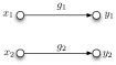
Figure 4: Parallel Channel Model for $2\times 2$ MIMO.

The channel can be written as,

$$\left[\begin{array}[]{c}y_{1}\\ y_{2}\end{array}\right]=\sqrt{\rho}\left[\begin{array}[]{cc}g_{1}&0\\ 0&g_{2}\end{array}\right]\left[\begin{array}[]{c}x_{1}\\ x_{2}\end{array}\right]+\left[\begin{array}[]{c}w_{1}\\ w_{2}\end{array}\right]$$

where $E[|x_{i}|^{2}]=1$, $w_{1},w_{2}\sim\mathcal{CN}(0,1)$. The capacity for $x_{i}\to y_{i}$ is given by $\log(1+\rho g_{i}^{2})$. It was shown in [6][2] that a D-BLAST transmission scheme with a MMSE successive interference cancellation receiver achieves the mutual information of the MIMO channel. For this scheme $g_{1}^{2}$ and $g_{2}^{2}$ can be calculated to be,

$$g_{2}^{2} = ||\mathbf{h}_{r\perp s}||^{2}+\frac{||\mathbf{h}_{r\parallel s}||^{2}}{1+\rho||\mathbf{h}_{s}||^{2}}$$

$$g_{1}^{2} = ||\mathbf{h}_{s}||^{2}$$

where $\mathbf{h}_{r\perp s}$ and $\mathbf{h}_{r\parallel s}$ respectively denote the perpendicular and parallel components of $\mathbf{h}_{r}$ with respect to $\mathbf{h}_{s}$.

Note that while $g_{1}^{2}$ and $g_{2}^{2}$ are correlated, $\mathbf{h}_{s},\mathbf{h}_{r\perp s}$ and $\mathbf{h}_{r\parallel s}$ are mutually independent. The correlation between $g_{1}^{2}$ and $g_{2}^{2}$ can therefore be explicitly calculated. The destination decodes $\mathbf{X}_{R}$ in the presence of interference from $\mathbf{X}_{S}^{2}$. It then cancels $\mathbf{X}_{R}$ from its received signal before decoding $\mathbf{X}_{S}^{2}$. Therefore $S$ effectively sees an interference free channel (with gain $g_{1}$) to $D$ during both listen and cooperation phases.

$$I_{\mathcal{C}_{D}}^{{}^{\prime}} = f\log(1+\rho g_{1}^{2})$$

$$+(1-f)[\log(1+\rho g_{1}^{2})+\log(1+\rho g_{2}^{2})]$$

$$= \log(1+\rho g_{1}^{2})+(1-f)\log(1+\rho g_{2}^{2})$$

Let $\alpha_{sr},\alpha_{1}$ and $\alpha_{2}$ represent channel realizations via the following variable transformations.

$$\alpha_{sr} = \lim_{\rho\to\infty}\frac{\log(1+\rho^{\eta}|h_{sr}|^{2})}{\log{\rho}}$$

$$\alpha_{1} = \lim_{\rho\to\infty}\frac{\log(1+\rho g_{1}^{2})}{\log{\rho}}$$

$$\alpha_{2} = \lim_{\rho\to\infty}\frac{\log(1+\rho g_{2}^{2})}{\log{\rho}}$$

This gives us simplified expressions for mutual information upper bounds.

$$\frac{I_{\mathcal{C}_{S}}^{{}^{\prime}}}{\log\rho} = \alpha_{1}+f(\alpha_{sr}-\alpha_{1})^{+}$$ (5)

$$\frac{I_{\mathcal{C}_{D}}^{{}^{\prime}}}{\log\rho} = \alpha_{1}+(1-f)\alpha_{2}$$ (6)

To achieve desired multiplexing gain $r$ at high SNR ($\rho\to\infty$) the network must achieve a rate $\mathcal{R}=r\log\rho$. The network is in outage if, $\min\{I_{\mathcal{C}_{S}}^{{}^{\prime}},I_{\mathcal{C}_{D}}^{{}^{\prime}}\}\leq r\log\rho$. For a given $r$ and schedule $f$ we can define the outage region $\mathcal{O}(r,f)$ over channel realizations $\vec{\alpha}=(\alpha_{1},\alpha_{2},\alpha_{sr})$.

$$\mathcal{O}(r,f)=\{\vec{\alpha}|\frac{\min\{I_{\mathcal{C}_{S}}^{{}^{\prime}},I_{\mathcal{C}_{D}}^{{}^{\prime}}\}}{\log\rho}\leq r\}$$ (7)

The outage probability $\mathcal{P}_{out}$ is,

$$\mathcal{P}_{out}=\int_{\vec{\alpha}\in\mathcal{O}(r,f)}f_{\vec{\alpha}}(\alpha_{1},\alpha_{2},\alpha_{sr})$$

where $f_{\vec{\alpha}_{1}}(\alpha_{1},\alpha_{2},\alpha_{sr})$ is the joint distribution of $(\alpha_{1},\alpha_{2},\alpha_{sr})$.

Lemma III.3

Proof see Appendix A

$$f_{\vec{\alpha}}(\alpha_{1},\alpha_{2},\alpha_{sr})\doteq\rho^{-s(\vec{\alpha})}$$

where $0\leq\alpha_{1},\alpha_{2}\leq 1$, $0\leq\alpha_{sr}\leq\eta$ and

$$s(\vec{\alpha})=\left\{\begin{array}[]{cc}\eta+4-3\alpha_{1}-2\alpha_{2}-\alpha_{sr}&\alpha_{1}+\alpha_{2}\leq 1\\ \eta+3-2\alpha_{1}-\alpha_{2}-\alpha_{sr}&\alpha_{1}+\alpha_{2}>1\end{array}\right.$$ (8)

For a given listen-transmit schedule $f$ the cut-set DMT bound is therefore given by,

$$d(r,f)=\min_{\vec{\alpha}\in\mathcal{O}(r,f)}s(\vec{\alpha})$$ (9)

To get the DMT upper bound we can optimize over all listen-transmit schedules,

$$d(r)=\min_{\vec{\alpha}\in\mathcal{O}(r)}\max_{f}s(\vec{\alpha})$$ (10)

Note that this optimization is performed on a per realization basis, i.e. the optimal $f$ depends on all channel realizations $\alpha_{sr},\alpha_{1}$ and $\alpha_{2}$. Therefore this corresponds to the global strategy discussed in Sec II.

It is easy to see that the globally optimal schedule $f_{glob}$ is one which sets $I_{\mathcal{C}_{S}}^{{}^{\prime}}=I_{\mathcal{C}_{D}}^{{}^{\prime}}$.

$$f_{glob}=\frac{\alpha_{2}}{(\alpha_{sr}-\alpha_{1})^{+}+\alpha_{2}}$$

This leads to the solution for $d(r)$ given in (1).

IV Achievability: Relaying Scheme

The “quantize-map” relaying scheme proposed in [7] and [8] has been shown to be DMT optimal for the single antenna relay channel [5]. We show that “quantize-map” adapts naturally to the network described in Sec II and with some modification achieves the cut-set DMT bound. For the sake of completeness we include a short description of the scheme.

IV-A Description of scheme

$S$ has a sequence of messages $w_{n}\in\{1,2,\ldots,2^{T\mathcal{R}}\}$, $n=1,2,\ldots$ to be transmitted. At both source $S$ and relay we create random Gaussian codebooks. $S$ randomly maps each message to one of its Gaussian codewords and transmits it using $T$ symbol times giving an overall transmission rate of $\mathcal{R}$. Due to the half-duplex nature of the relay, it must operate using listen-transmit cycles. Relay listens to the first $fT$ time symbols of each block i.e. $\mathbf{X}_{S}^{1}$. It quantizes $\mathbf{Y}_{R}$ to $\hat{\mathbf{Y}}_{R}$ and then randomly maps it into a Gaussian codeword $\mbox{${\bf X}$}_{R}$ using a random mapping function $f_{R}(\hat{\mbox{${\bf Y}$}}_{R})$. It transmits this codeword during the next $(1-f)T$ symbol times. Given the knowledge of all the encoding functions and signals received, $D$ attempts to decode the message sent by $S$.

IV-B DMT of Quantize-Map

By Theorem 7.4.1 in [8], for any fixed listen-transmit schedule $f$, the quantize-map relaying scheme, uniformly over all channel realizations achieves a rate within a constant gap to the cut-set upper bound $\min\{I_{\mathcal{C}_{S}}^{{}^{\prime}},I_{\mathcal{C}_{D}}^{{}^{\prime}}\}$ for that particular $f$. The random Gaussian code-book generated at source is independent of $f$. Also the code-book generated at relay depends on $f$ only to determine the length of each codeword $(1-f)T$.

The relay can generate a larger code-book with each codeword of length $T$. If the relay now chooses a listen-transmit schedule $f$, it can use the first $(1-f)T$ symbols of the codeword to compose $\mbox{${\bf X}$}_{R}$. The destination always knows the schedule $f$ and hence can adapt its decoder accordingly. This construction allows us to claim that “quantize-map” achieves a rate within a constant gap of $\min\{I_{\mathcal{C}_{S}}^{{}^{\prime}},I_{\mathcal{C}_{D}}^{{}^{\prime}}\}$ uniformly for each dynamic choice of $f$ i.e.

$$\min\{I_{\mathcal{C}_{S}}^{{}^{\prime}},I_{\mathcal{C}_{D}}^{{}^{\prime}}\}-\kappa\leq R_{\text{quantize-map}}(h_{sr},\mathbf{h}_{s},\mathbf{h}_{r},\rho,f)$$ (11)

The constant $\kappa$ in the above equation does not depend on the channel gains and SNR. At the order of DMT which assumes high SNR $(\rho\to\infty)$ the effect of $\kappa$ becomes negligible and hence we have the following theorem for achievability.

Theorem IV.1

For dynamic listen-transmit schedules, the modified quantize-map relaying scheme as described above achieves the diversity multiplexing tradeoff of $\min\{I_{\mathcal{C}_{S}}^{{}^{\prime}},I_{\mathcal{C}_{D}}^{{}^{\prime}}\}$, where $I_{\mathcal{C}_{S}}^{{}^{\prime}}$ and $I_{\mathcal{C}_{D}}^{{}^{\prime}}$ are given by (5)(6).

V Achievability: Listen-Transmit Schedule

In Sec III-A the cut-set DMT upper bound was calculated for the globally optimal listen-transmit schedule $f_{glob}$. However in a practical communication scenario global knowledge of instantaneous channel realizations may not be available at the relay. To account for this we defined the local and blind relaying strategies in Sec II. In this section we refine Theorem III.1 to calculate DMT bounds for local and blind schedules.

V-A Blind Scheduling

Theorem V.1

For the low rate region i.e. $r\leq 1$, the blind scheduling strategy is DMT optimal. Additionally for $\eta\geq 2$ the blind strategy achieves the $2\times 2$ MIMO DMT bound for $r\leq 1$. The optimal blind schedule for this region is $f_{blind}=\frac{1}{3}$

$$\begin{array}[]{cc}d_{blind}(r)=\min\{\eta+2,4\}-3r&r\leq 1\end{array}$$ (12)

Figure 5: $d(r)$ $d_{local}(r)$ and $d_{blind}(r)$ comparison for $r\geq 1$.

From (9) the DMT bound for blind scheduling can be written as,

$$d_{blind}(r)=\max_{f}\min_{\vec{\alpha}\in\mathcal{O}(r,f)}s(\vec{\alpha})$$ (13)

i.e. $f$ is optimized without knowledge of channel realizations $\vec{\alpha}$. Solving this optimization for $r\leq 1$ yields Theorem V.1. This suggests that as long as cooperative multiplexing is not necessary i.e. desired rate $\mathcal{R}=r\log(\rho)$ is such that $r\leq 1$, static scheduling at relay is sufficient to achieve the DMT upper bound. $f_{blind}=\frac{1}{3}$ turns out to be the optimal listen-transmit schedule for this region.

For the high rate region $(r>1)$, the analytical solution for (13) is tedious to obtain. The optimization is convex and can be solved numerically. Figure 5 shows a comparison between $d(r)$ and $d_{blind}(r)$ for $r\geq 1$. It can be seen that for cooperative multiplexing $(r\geq 1)$ static scheduling is insufficient to achieve DMT upper bound.

V-B Local Scheduling

Similarly, the DMT bound for local scheduling can be expressed as an optimization problem from (9).

$$d_{local}(r)=\min_{\alpha_{sr}}\max_{f}\min_{\alpha_{1},\alpha_{2}\in\mathcal{O}(r,f)}s(\vec{\alpha})$$ (14)

$f_{local}$ can be optimized using knowledge of $\alpha_{sr}$ only. The DMT performance of local scheduling must be at-least as good as blind scheduling, therefore by Theorem V.1 for $r\leq 1$ $d_{local}(r)=d_{blind}(r)=d(r)$.

Numerical solution to (14) for the high rate $r\geq 1$ region is shown in Figure 5. It can be seen that local scheduling performs better than blind, but for higher $\eta$ this advantage diminishes.

VI Acknowledgements

The authors wish to acknowledge the contributions of the students, faculty and sponsors of the Berkeley Wireless Research Center and the National Science Foundation Infrastructure Grant No. 0403427.

Appendix A Proof of Lemma 8

A-A Marginal Distribution of $\alpha_{sr}$

$f_{\alpha_{sr}}(\alpha)$ is calculated as,

$$\mathcal{P}[\alpha_{sr}<\alpha] = \lim_{\rho\to\infty}\mathcal{P}[|h_{sr}|^{2}<\rho^{\alpha_{sr}-\eta}]$$

$$f_{\alpha_{sr}}(\alpha) \doteq \rho^{\eta-\alpha}(0\leq\alpha_{sr}\leq\eta)$$

A-B Joint Distribution of $\alpha_{1}$ and $\alpha_{2}$

Note that $g_{1}^{2}$ has a $\chi^{2}_{4}$ distribution, the marginal distribution of $\alpha_{1}$ is given by,

$$f_{\alpha_{1}}(\alpha_{1}) =f_{g_{1}^{2}}(\rho^{-(1-\alpha_{1})})\frac{dg_{1}^{2}}{d\alpha_{1}}$$

$$\doteq\rho^{-2(1-\alpha_{1})}(0\leq\alpha_{1}\leq 1)$$

Now for $(0\leq\alpha_{1},\alpha_{2}\leq 1)$ their joint CDF can be written as,

$$F_{\alpha_{1},\alpha_{2}}(\alpha_{1},\alpha_{2}) = \mathcal{P}[g_{1}^{2}\leq\rho^{\alpha_{1}-1},g_{2}^{2}\leq\rho^{\alpha_{2}-1}]$$

$$= \int_{x=0}^{\alpha_{1}}\mathcal{P}[g_{1}^{2}=\rho^{x-1},g_{2}^{2}\leq\rho^{\alpha_{2}-1}]dx$$

$$\doteq \int_{x=0}^{\alpha_{1}}\rho^{-2(1-x)}$$

$$\mathcal{P}(|h_{s\perp r}|^{2}+\frac{|h_{s\parallel r}|^{2}}{1+\rho^{x}}\leq\rho^{\alpha_{2}-1})dx$$

$$\doteq \int_{x=0}^{\alpha_{1}}\rho^{-2(1-x)}$$

$$\int_{y=0}^{\alpha_{2}-1}\rho^{y}\mathcal{P}(|h_{s\parallel r}|^{2}\dot{\leq}\rho^{x+\alpha_{2}-1})\ dy\ dx$$

A-B1 Case $\alpha_{1}+\alpha_{2}\leq 1$

$$F_{{\alpha_{1},\alpha_{2}}}(\alpha_{1},\alpha_{2}) \doteq \int_{x=0}^{\alpha_{1}}\rho^{-2(1-x)}\int_{y=0}^{\alpha_{2}-1}\rho^{x+y+\alpha_{2}-1}\ dy\ dx$$

$$\doteq \int_{x=0}^{\alpha_{1}}\rho^{3x+2\alpha_{2}-4}\ dx$$

$$\doteq \rho^{3\alpha_{1}+2\alpha_{2}-4}$$

$$f_{\alpha_{1},\alpha_{2}}(\alpha_{1},\alpha_{2}) \doteq \rho^{3\alpha_{1}+2\alpha_{2}-4}$$

A-B2 Case $\alpha_{1}+\alpha_{2}>1$

$$F_{{\alpha_{1},\alpha_{2}}}(\alpha_{1},\alpha_{2}) \doteq \int_{x=0}^{1-\alpha_{2}}\rho^{3x+2\alpha_{2}-4}\ dx$$

$$+\int_{x=1-\alpha_{2}}^{\alpha_{1}}\rho^{2x+\alpha_{2}-3}\ dx$$

$$\doteq \rho^{2\alpha_{2}+\alpha_{1}-3}$$

$$f_{\alpha_{1},\alpha_{2}} \doteq \rho^{2\alpha_{1}+\alpha_{2}-3}$$

Since $\alpha_{sr}$ is independent of $\alpha_{1},\alpha_{2}$ we get Lemma 8.

References

• [1] Y.ย Fan, H.ย V. Poor, and J.ย S. Thompson, โ€œCooperative multiplexing in full-duplex multi-antenna relay networks,โ€ Global Telecommunications Conference, 2008. IEEE GLOBECOM 2008. IEEE, pp. 1โ€“5, 30 2008-Dec. 4 2008.
• [2] L.ย Zheng and D.ย Tse, โ€œDiversity and multiplexing: a fundamental tradeoff in multiple-antenna channels,โ€ Information Theory, IEEE Transactions on, vol.ย 49, no.ย 5, pp. 1073โ€“1096, May 2003.
• [3] J.ย Laneman, D.ย Tse, and G.ย Wornell, โ€œCooperative diversity in wireless networks: Efficient protocols and outage behavior,โ€ Information Theory, IEEE Transactions on, vol.ย 50, no.ย 12, pp. 3062โ€“3080, Dec. 2004.
• [4] M.ย Yuksel and E.ย Erkip, โ€œMultiple-antenna cooperative wireless systems: A diversityโ€“multiplexing tradeoff perspective,โ€ Information Theory, IEEE Transactions on, vol.ย 53, no.ย 10, pp. 3371โ€“3393, Oct. 2007.
• [5] S.ย Pawar, A.ย Avestimehr, and D.ย Tse, โ€œDiversity-multiplexing tradeoff of the half-duplex relay channel,โ€ in Proc. Forty-Sixth Allerton Conf. Commun. Contr. Comput., Illinois, 2008.
• [6] M.ย Varanasi and T.ย Guess, โ€œOptimum decision feedback multiuser equalization with successive decoding achieves the total capacity of the gaussian multiple-access channel,โ€ Signals, Systems and Computers, 1997. Conference Record of the Thirty-First Asilomar Conference on, vol.ย 2, pp. 1405โ€“1409, Nov 1997.
• [7] A.ย Avestimehr, S.ย Diggavi, and D.ย Tse, โ€œApproximate capacity of gaussian relay networks,โ€ Information Theory, 2008. ISIT 2008. IEEE International Symposium on, pp. 474โ€“478, July 2008.
• [8] A.ย S. Avestimehr, โ€œWireless network information flow: a deterministic approach,โ€ Ph.D. dissertation, EECS Department, University of California, Berkeley, Oct 2008. [Online]. Available: http://www.eecs.berkeley.edu/Pubs/TechRpts/2008/EECS-2008-128.html