A WENO algorithm for radiative transfer with resonant scattering and the Wouthuysen-Field Coupling

Abstract

We develop a numerical solver for the integral-differential equations, which describe the radiative transfer of photon distribution in the frequency space with resonant scattering of Ly$\alpha$ photons by hydrogen gas in the early universe. The time-dependent solutions of this equation is crucial to the estimation of the effect of the Wouthuysen-Field (WF) coupling in relation to the 21 cm emission and absorption at the epoch of reionization. However, the time-dependent solutions of this equation have not yet been well performed. The resonant scattering leads to the photon distribution in the frequency space to be piecewise smooth containing sharp changes. The weighted essentially nonoscillatory (WENO) scheme is suitable to handle this problem, as this algorithm has been found to be highly stable and robust for solving Boltzmann equation. We test this numerical solver by 1.) the analytic solutions of the evolution of the photon distribution in rest background; 2.) the analytic solution in expanding background, but without resonant scattering; 3.) the formation of local Boltzmann distribution around the resonant frequency with the temperature to be the same as that of atom for recoil. We find that the evolution of the photon distribution due to resonant scattering with and without recoil generally undergoes three phases. First, the profile of the photon distribution is similar to the initial one. Second, an extremely flat plateau (without recoil) or local Boltzmann distribution (with recoil) form around the resonant frequency, and the width and height of the flat plateau or local Boltzmann distribution increase with time. Finally, the distribution around the resonant frequency is saturated when the photons from the source is balanced by the redshift of the expansion. This result indicates that the onset of the W-F coupling should not be determined by the third phase, but by the time scale of the second phase. We found that the time scale of the W-F coupling is equal to about a few hundreds of the mean free flight time of photons with resonant frequency, and it basically is independent of the Sobolev parameter if this parameter is much less than 1.

, , ,

1 Introduction

It is generally believed that detecting redshifted 21 centimeter signals from early universe is one of the next frontiers in observational cosmology, because it would be able to provide the information of the first generation of light sources in the cosmic dark ages. Many studies have been done on the 21 cm emission and absorption from the halo of individual first stars (Chuzhoy et al. 2006, Cen 2006, Liu et al. 2007). A common conclusion of these works is that the configurations of the 21 cm emission and absorption regions is strongly time-dependent. The reason is simple. The necessary conditions of 21 cm emission and absorption are that 1. the fraction of neutral hydrogen (HI) is still high; 2, Ly$\alpha$ photons are available for the Wouthuysen-Field (W-F) coupling. The region of 21 cm emission around first stars is then a thin shell just outside the I-front (ionization-front). Hence the 21 cm emission shell should move with a speed higher than the speed of the I-front $v_{f}$, which is rather high, even comparable to the speed of light. Therefore, the time scale of the formation and evolution of the regions of 21 cm signal can roughly be estimated by $d/v_{f}$, $d$ being the thickness of the 21 cm emission and absorption shell. This time scale is found to be of the order of 1 Myr and less (Cen 2006, Liu et al. 2007).

In all of the above-mentioned works, the spin temperature is calculated with the assumption that the Wouthuysen-Field (W-F) coupling (Wouthuysen, 1952; Field, 1958, 1959) is effective. That is, the color temperature of photons around Ly$\alpha$ frequency is assumed to be the same as the kinetic temperature of hydrogen gas. The W-F coupling locks the color temperature of Ly$\alpha$ photon to the kinetic temperature of hydrogen gas, and then links the internal (spin-) degree of freedom with the kinetic temperature of gas. Obviously, the W-F coupling would be available if the time scale of the onset of the W-F coupling is less than the time scale of the formation and evolution of the 21 cm emission and absorption shells. However, most calculations on the W-F coupling are based on the time-independent Fokker-Planck approximation (Chen & Miralda-Escude, 2004; Hirata, 2006; Furlanetto & Pritchard 2006; Chuzhoy & Shapiro 2006) of the radiative transfer with resonant scattering of Ly$\alpha$ photons by hydrogen gas. The time-independent solution is acceptable only if the time-independent state is approached in a scale shorter than that of the evolution of the 21 cm signal regions. Unfortunately, this assumption is not obvious. Time-dependent solutions are necessary.

The W-F coupling is due to the resonant scattering of Ly$\alpha$ photons by hydrogen atoms. It is described by a Boltzmann-like integro-differential equation of radiative distribution in the phase space. The W-F coupling is sensitive to the evolution of the photon distribution in the frequency space. The analytical solutions of this equation with resr background has revealed that the frequency distribution of photons under the resonant scattering of Ly$\alpha$ photons by gaseous hydrogen atoms without recoil has two features: 1. an extremely flat top of the photon profiles in the frequency space; 2. a sharp boundary of the flat top range(Field 1958). Currently, the numerical results are still far from precise to match these features (e.g. Meiksin, 2006).

In this paper, we develop a numerical solver with the weighted essentially nonoscillatory (WENO) scheme. The WENO method has high order of accuracy and good convergence in capturing discontinuities as well as to be significantly superior over piecewise smooth solutions containing discontinuities (Shu 2003). WENO schemes have been widely used in applications. It is also effective in solving Boltzmann equations (Carrillo et al. 2003, 2006) and radiative transfer (Qiu et al. 2006, 2007, 2008). Therefore, one can expect that the integral-differential equations of resonant scattering can be properly handled numerically by the WENO scheme.

The paper is organized as follows. Section 2 presents the basic equations of the resonant scattering of radiation. Section 3 gives the numerical solver of the WENO scheme. Section 4 presents the tests of the numerical solver. The time scale of the W-F coupling is briefly addressed in Section 5. A discussion and conclusion are given in Section 6.

2 Basic equations

2.1 Radiative transfer equations with resonant scattering

Considering a spatially homogeneous and isotropically expanding infinite medium consisting of neutral hydrogen with temperature $T$, the kinetics of photons in the frequency space is described by the radiative transfer equation with resonant scattering (Hummer & Rybicki, 1992; Rybicki & Dell’antonio 1994)

$$\frac{\partial J(x,t)}{\partial t}+2HJ(x,t)-\frac{cH}{v_{T}}\frac{\partial J(x,t)}{\partial x}=$$

$$-kc\phi(x)J(x,t)+kc\int\mathcal{R}(x,x^{\prime})J(x^{\prime},t)dx^{\prime}+C(t)\phi(x)$$ (1)

where $J$ is the specific intensity in terms of the photon number, $H(t)=\dot{R}(t)/R(t)$ is the Hubble parameter, $R(t)$ is the cosmic factor, $v_{T}=(2k_{B}T/m)^{1/2}$ is the thermal velocity of hydrogen atom, the dimensionless frequency $x$ is related to the frequency $\nu$ and the resonant frequency $\nu_{0}$ by $x=(\nu-\nu_{0})/\Delta\nu_{D}$, and $\Delta\nu_{D}=\nu_{0}v_{T}/c$ is the Doppler broadening. The parameter $k=\chi/\Delta\nu_{D}$, and the intensity of the resonant absorption $\chi$ is given by $\chi=\pi e^{2}n_{1}f_{12}/m_{e}c$, where $n_{1}$ the number density of neutral hydrogen HI at ground state, and $f_{12}=0.416$ is the oscillation strength. The cross section at the line center is

$$\sigma_{0}=\frac{\pi e^{2}}{m_{e}c}f_{12}(\Delta\nu_{D})^{-1}.$$ (2)

In eq.(2.1), $C(t)$ is the source of photons with the frequency distribution $\phi(x)$, which is the Voigt function of the frequency profile with the center at $\nu_{0}$, i.e.

$$\phi(x)=\frac{a}{\pi^{3/2}}\int^{\infty}_{-\infty}dy\frac{e^{-y^{2}}}{(x-y)^{2}+a^{2}}$$ (3)

where $a$ is the ratio of the natural to the Doppler broadening. We have $a=A_{21}/(8\pi\Delta\nu_{D})$, and $A_{21}=6.25\times 10^{8}$ Hz is the Einstein spontaneous emission coefficient. $\phi(x)$ is normalized with $\displaystyle\int\phi(x^{\prime})dx^{\prime}=1$. When $a\rightarrow 0$, we have pure Doppler broadening as

$$\phi_{D}(x)=\frac{1}{\sqrt{\pi}}e^{-x^{2}}.$$ (4)

The redistribution function $\mathcal{R}(x,x^{\prime})$ gives the probability of a photon absorbed at the frequency $x^{\prime}$, and re-emitted at the frequency $x$. It depends on the details of the scattering (Henyey 1941; Hummer 1962; Hummer, 1969). If we consider coherent scattering without recoil, it is

$$\mathcal{R}(x,x^{\prime})=$$

$$\frac{1}{\pi^{3/2}}\int^{\infty}_{|x-x^{\prime}|/2}e^{-u^{2}}\left[\tan^{-1}\left(\frac{x_{\min}+u}{a}\right)-\tan^{-1}\left(\frac{x_{\max}-u}{a}\right)\right]du$$

where $x_{\min}=\min(x,x^{\prime})$ and $x_{\max}=\max(x,x^{\prime})$. Obviously, $\displaystyle\int_{-\infty}^{\infty}\mathcal{R}(x,x^{\prime})dx^{\prime}=\phi(x)$. In the case of $a=0$, i.e. considering only the Doppler broadening, eq.(2.1) becomes

$$\mathcal{R}(x,x^{\prime})=\frac{1}{2}{\rm erfc}[{\rm max}(|x|,|x^{\prime}|)].$$ (6)

Considering the recoil of atoms, the redistribution function for the Doppler broadening is (Field, 1959, Basko, 1981)

$$\mathcal{R}(x,x^{\prime})=\frac{1}{2}e^{2bx^{\prime}+b^{2}}{\rm erfc}[{\rm max}(|x+b|,|x^{\prime}+b|)],$$ (7)

where parameter $b=h\nu_{0}/mv_{T}c=2.5\times 10^{-4}(10^{4}/T)^{1/2}$.

2.2 Re-scaling the equations

We use the new time variable $\tau$ defined as $\tau=cn_{1}\sigma_{0}t$, which is in units of the mean free flight time of photons at resonant frequency. The number density of neutral hydrogen atoms $n_{1}=f_{\rm HI}n_{\rm H}$, with $f_{\rm HI}$ being the fraction of neutral hydrogen. For the concordance $\Lambda$CDM model, we have $n_{\rm H}=1.88\times 10^{-7}(\Omega_{b}h^{2}/0.02)(1+z)^{3}$ cm^-3. The factor 0.75 is from hydrogen abundance. Therefore,

$$t=0.054\tau f^{-1}_{\rm HI}\left(\frac{T}{10^{4}}\right)^{1/2}\left(\frac{10}{1+z}\right)^{3}\left(\frac{0.022}{\Omega_{b}h^{2}}\right)\hskip 8.53581ptyrs$$ (8)

We re-scale the eq.(2.1) by the following new variables

$$J^{\prime}(x,t)=[R(t)/R_{0}]^{2}J,\hskip 14.22636ptC^{\prime}(t)=[R(t)/R_{0}]^{2}C.$$ (9)

Thus, eq.(2.1) becomes

$$\frac{\partial J^{\prime}(x,\tau)}{\partial\tau} = -\phi(x)J^{\prime}(x,\tau)$$ (10)

$$+\int\mathcal{R}(x,x^{\prime})J^{\prime}(x^{\prime},\tau)dx^{\prime}+\gamma\frac{\partial J^{\prime}}{\partial x}+C^{\prime}(\tau)\phi(x).$$

We will use $J$ for $J^{\prime}$ and $C$ for $C^{\prime}$ in the equations below. The parameter $\gamma$ is the so-called Sobolev parameter, $\gamma=(H/v_{T}k)=(8\pi H/3A_{12}\lambda^{3}n_{1})=(Hm_{e}\nu_{0}/\pi e^{2}n_{1}f_{12})$, where $\lambda$ is the wavelength for Ly$\alpha$ transition. $\gamma$ is simply related to the Gunn-Peterson optical depth $\tau_{GP}$ by

$$\gamma^{-1}=\tau_{GP}=4.9\times 10^{5}h^{-1}f_{\rm HI}\left(\frac{0.25}{\Omega_{M}}\right)^{1/2}\left(\frac{\Omega_{b}h^{2}}{0.022}\right)\left(\frac{1+z}{10}\right)^{3/2}.$$ (11)

The redshift evolution of $f_{\rm HI}$ is dependent on the reionization models. Before reionization $f_{\rm HI}\simeq 1$; after reionization $f_{\rm HI}\simeq 10^{-5}$ in average. Therefore, the parameter $\gamma$ has to be in the range from 1 ($z\leq 7$) to $10^{-7}$ ($z\geq 10$). For static background, $\gamma=0$.

3 Numerical solver: the WENO scheme

3.1 Computational domain and computational mesh

The computational domain in the case of static background is $x\in[-6,6]$. The initial condition is $J(x,0)=0$. The boundary condition is

$$J(x,\tau)=0,\ {\rm\ at\ }|x|=6.$$ (12)

In the case of expanding background, i.e.$\gamma\neq 0$, the computational domain is bigger than $x\in[-6,6]$ depending on the value of the Sobolev parameter $\gamma$. The domain $(x_{left},x_{right})$ is chosen such that for the particular value of $\gamma$ we have

$$J(x_{left},\tau)\approx 0,\quad J(x_{right},\tau)\approx 0.$$ (13)

For example, the domain is taken to be $x\in[-100,6]$ for the case of $\gamma=10^{-3}$. Also for different values of $\gamma$ the solutions reach saturation at different time. For example, we see in our numerical results that the solution $J(\nu,t)$ of eq. (9) reaches saturation at time $\tau=100$ for $\gamma=10^{-1}$, and reaches saturation at time $\tau=10^{4}$ for $\gamma=10^{-3}$. The computational domain is discretized into a uniform mesh in the $x$ direction,

$$x_{i}=x_{left}+i\Delta x,\hskip 71.13188pti=0,1,2,\cdots,N_{x},$$

where $\Delta x=(x_{right}-x_{left})/N_{x}$, is the mesh size. We also denote $J_{i}^{n}=J(x_{i},\tau^{n})$, the approximate solution values at $(x_{i},\tau^{n})$.

3.2 Algorithm of the spatial derivative

To calculate $\frac{\partial J}{\partial x}$, we use the fifth order WENO method (Jiang & Shu, 1996). That is,

$$\frac{\partial J(x_{i},\tau^{n})}{\partial x}\approx\frac{1}{\Delta x}(\hat{h}_{j+1/2}-\hat{h}_{j-1/2}\\ )$$ (14)

where the numerical flux $\hat{h}_{j+1/2}$ is obtained by the procedure given below. We use the upwind flux in the fifth order WENO approximation because the wind direction is fixed (negative). First we denote

$$h_{i}=J(x_{i},\tau^{n}),\hskip 71.13188pti=-2,-1,\cdots,N_{x}+3\\$$ (15)

where $n$ is fixed. The numerical flux from the WENO procedure is obtained by

$$\hat{h}_{i+1/2}=\omega_{1}\hat{h}_{i+1/2}^{(1)}+\omega_{2}\hat{h}_{i+1/2}^{(2)}+\omega_{3}\hat{h}_{i+1/2}^{(3)},\\$$ (16)

where $\hat{h}_{i+1/2}^{(m)}$ are the three third order fluxes on three different stencils given by

$$\hat{h}_{i+1/2}^{(1)} = -\frac{1}{6}h_{i-1}+\frac{5}{6}h_{i}+\frac{1}{3}h_{i+1},$$

$$\hat{h}_{i+1/2}^{(2)} = \frac{1}{3}h_{i}+\frac{5}{6}h_{i+1}-\frac{1}{6}h_{i+2},$$

$$\hat{h}_{i+1/2}^{(3)} = \frac{11}{6}h_{i+1}-\frac{7}{6}h_{i+2}+\frac{1}{3}h_{i+3},$$

and the nonlinear weights $\omega_{m}$ are given by,

$$\omega_{m}=\frac{\check{\omega}_{m}}{\displaystyle\sum_{l=1}^{3}\check{\omega}_{l}},\hskip 14.22636pt\check{\omega}_{l}=\frac{\gamma_{l}}{(\epsilon+\beta_{l})^{2}},\\$$ (17)

where $\epsilon$ is a parameter to avoid the denominator to become zero and is taken as $\epsilon=10^{-8}$. The linear weights $\gamma_{l}$ are given by

$$\gamma_{1}=\frac{3}{10},\hskip 8.53581pt\gamma_{2}=\frac{3}{5},\hskip 8.53581pt\gamma_{3}=\frac{1}{10},$$ (18)

and the smoothness indicators $\beta_{l}$ are given by

$$\beta_{1} = \frac{13}{12}(h_{i-1}-2h_{i}+h_{i+1})^{2}+\frac{1}{4}(h_{i-1}-4h_{i}+3h_{i+1})^{2},$$

$$\beta_{2} = \frac{13}{12}(h_{i}-2h_{i+1}+h_{i+2})^{2}+\frac{1}{4}(h_{i}-h_{i+2})^{2},$$

$$\beta_{3} = \frac{13}{12}(h_{i+1}-2h_{i+2}+h_{i+3})^{2}+\frac{1}{4}(3h_{i+1}-4h_{i+2}+h_{i+3})^{2}.$$

3.3 High order numerical integration

The integration of the resonance scattering term is calculated by a fifth order quadrature formula (Shen et al. 2007)

$$\int_{x_{left}}^{x_{right}}f(x)dx=\Delta x\sum_{j=0}^{N_{x}}w_{j}f(x_{j})+O(\Delta x^{5}),\\$$ (19)

where the weights are defined as,

$$w_{0}=\frac{251}{720},\quad w_{1}=\frac{299}{240},\quad w_{2}=\frac{211}{240},\quad w_{3}=\frac{739}{720},$$

$$w_{N_{x}-3}=\frac{739}{720},\quad w_{N_{x}-2}=\frac{211}{240},\quad w_{N_{x}-1}=\frac{299}{240},w_{N_{x}}=\frac{251}{720},$$

and $w_{j}=1$ otherwise. Notice that this numerical integration is very costly and uses most part of the CPU time. For the equation with recoil and the redistribution function with $a=0$, we have used a grouping of the numerical integration operations at different $x$ locations so that the computational cost can be reduced to order $O(N)$ rather than $O(N^{2})$, where $N$ is the number of grid points in $x$, without changing mathematically the algorithm and its accuracy. The $O(N)$ algorithm for numerical integration is given in the appendix which further highlights the speed and accuracy of the numerical algorithm proposed in this paper. Unfortunately, this grouping technique does not work for the case $a\neq 0$, hence the CPU cost for the case with $a\neq 0$ is much larger.

3.4 Time evolution

To evolve in time, we use the third-order TVD Runge-Kutta time discretization (Shu & Osher, 1988). For systems of ODEs $u_{t}=L(u)$, the third order Runge-Kutta method is

$$u^{(1)} = u^{n}+\Delta\tau L(u^{n},\tau^{n}),$$

$$u^{(2)} = \frac{3}{4}u^{n}+\frac{1}{4}(u^{(1)}+\Delta\tau L(u^{(1)},\tau^{n}+\Delta\tau)),$$

$$u^{(3)} = \frac{1}{3}u^{n}+\frac{2}{3}(u^{(2)}+\Delta\tau L(u^{(2)},\tau^{n}+\frac{1}{2}\Delta\tau)).$$

4 Tests of the WENO solver

4.1 Static background

We first test the WENO solver with two analytical solutions of eq. (10) with static background, $H=\gamma=0$ and Doppler broadening $a=0$ (Field, 1958). The first analytical solution is for the initial radiative field $J(x,\tau)=0$ and the constant source $C(\tau)=1$. It is

$$J(x,\tau)=\pi^{-1/2}[1-\exp(-\tau e^{-x^{2}})]$$

$$\ \hskip 56.9055pt+\int_{x}^{\infty}e^{w^{2}}[1-(1+\tau e^{-w^{2}})\exp(-\tau e^{-w^{2}})]{\rm erf}(w)dw.$$

The second analytical solution of eq.(10) is also for $H=\gamma=0$, $a=0$, but the source $C=0$, while the initial radiative field is

$$J(\nu,0)=\pi^{-1/2}e^{-\nu^{2}}.$$ (21)

The solution is

$$J(x,\tau)=\pi^{-1/2}e^{-x^{2}}\exp(-\tau e^{-x^{2}})+\tau\int_{x}^{\infty}e^{-w^{2}}\exp(-\tau e^{-w^{2}}){\rm erf}(w)dw.$$ (22)

The analytical solutions (4.1) and (22) are shown in Figures 1 and 2 respectively. We also plot the numerical solutions given by our algorithm in same figures. The numerical results show very small deviation from the analytical solutions.

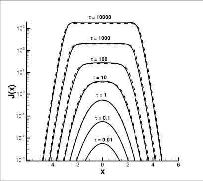
Figure 1: Static solutions ($\gamma=0$) for pure Doppler redistribution ($a=0$) of eq.(10), in which $C=1$ and $J(x,0)=0$. The analytical solutions are shown by dashed lines, while the numerical results are shown by solid lines.

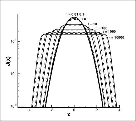
Figure 2: Static solutions ($\gamma=0$) for pure Doppler redistribution ($a=0$) of eq.(10), in which $C=0$ and $J(x,0)=\pi^{-1/2}\exp(-x^{2})$. The analytical solutions are shown by dashed line, while the numerical results are shown by solid lines.

A common feature of Figures 1 and 2 is that the originally Doppler peak at the center of the frequency profile gradually becomes a flat plateau. The width of the plateau increases with time. This is because the resonant scattering makes a non-uniform distribution in the frequency space to a uniform one. It is similar to that in the physical space, diffusion generally leads to an evolution from non-uniform distribution to a uniform one. The height of the plateau of Figure 1 is increasing with time, while in Figure 2 it is decreasing, because for the case $C=1$, the number of photons increases, while for the case of $C=0$, the total number of photons is conserved.

4.2 Expanding background

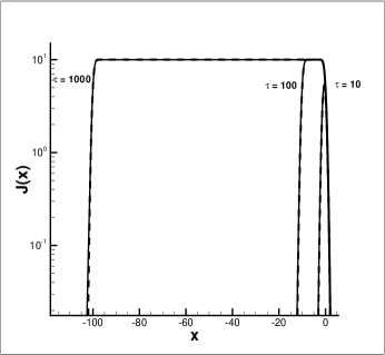
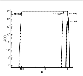
Figure 3: Solutions of $J(x,\tau)$ of eq.(23) with initial condition $J(x,0)=0$. The parameter $\gamma$ is taken to be $10^{-1}$ (left panel) and $10^{-3}$ (right). The analytical solutions eq.(24) are shown by dashed lines

.

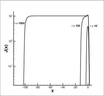
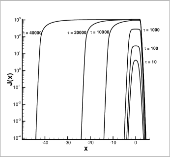
Figure 4: Solutions of $J(x,\tau)$ of eq.(10) with initial condition $J(x,0)=0$. The parameter $\gamma$ is taken to be $10^{-1}$ (left) and $10^{-3}$ (right).

The second test is given by considering expanding background. Without absorption and scattering, eq.(10) becomes

$$\frac{\partial J}{\partial\tau}=\gamma\frac{\partial J}{\partial x}+C(\tau)\phi(x).$$ (23)

If $C$ is $\tau$-independent, the analytic solution of eq.(23) is (Rybicki & Dell’antonio, 1994)

$$J(x,\tau)=J(x+\gamma\tau,0)+C\gamma^{-1}[\Phi(x)-\Phi(x+\gamma\tau)]$$ (24)

where

$$\Phi(x)=\int_{x}^{\infty}\phi(x^{\prime})dx^{\prime}$$ (25)

The meaning of the solution eq.(24) is simple. It just shows that the redshift of photons in frequency space is described by

$$-x=\gamma\tau.$$ (26)

We take $\phi(x)=(1/\sqrt{\pi})e^{-x^{2}}$, and assuming the initial field $J(x,0)=0$. Figure 3 shows that the numerical results obtained by using the WENO algorithm agree well with the analytic solution of eq.(24).

Figure 4 is the solutions of eq.(10) with parameter $\gamma=10^{-1}$ and $10^{-3}$. In these cases the analytical solutions are not available. We can see from Figure 3 and 4 that the intensity $J$ stops to increase and approaches a saturated value when $\tau$ is large. This happens when the number of photons produced from the sources is equal to that of the redshifted photons.

4.3 The effect of recoil of atom

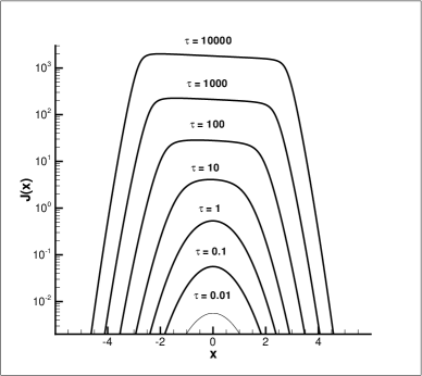
Figure 5: Solutions of $J(x,\tau)$ of eq.(10) with redistribution function eq.(7), and $\gamma=0$.

The third test is by using the redistribution function with recoil Eq.(7). Figure 5 gives the solutions of eq.(10) with parameter $b=0.03$, and the initial condition and source term are taken to be the same as Figure 1. The results of Figure 5 actually is similar to Figure 1, but only the center flat plateau of Figure 1 now is replaced by a sloping plateau. The latter is a local Boltzmann distribution around the renasont scattering.

Field (1959) has shown that, once the solution $J(x,\tau)$ of eq.(10) with $b=0$ has a flat plateau in the central region, the effect of recoil is to make the flat plateau to be a Boltzmann-like distribution, i.e. if the solution with no recoil redistribution eq.(6) shows $J(x,\tau)\simeq J(0,\tau)$, within $|x|<x_{f}$, the solution of eq.(10) with redistribution eq.(23) will be

$$J(0,\tau)e^{-2bx}=J(0,\tau)e^{-h(\nu-\nu_{0})/kT},\hskip 14.22636pt|x|<x_{f}.$$ (27)

One can test this property with $F(\tau)$ defined as

$$F(\tau)=\log J(0,\tau)-\log(1,\tau)$$ (28)

If the local Boltzmann distribution within $|x|<1$ is realized at time $\tau$, $F(\tau)$ should be equal to $2b$ [eq.(27)]. In Figure 6, we present the relation of $F(\tau)$ vs. $\tau$. At $\tau=0$, the Gaussian sources [eq.(21)] yields $F(0)=1$. Then, $F(\tau)$ approaches to $2b$ at $\tau>10^{2}$. These results show that the WENO solver is reliable and effective to study the time-dependence of $J$ described by the resonant scattering equation.

Figure 6 also shows the relation $F(\tau)$ vs. $\tau$ for solutions $b=0.03$ (left panel) and $b=0$ (right panel). The two curves actually are similar. When the right curve approaches to $F(\tau)\rightarrow 0$ at time $\tau$, the left curve, at the same time, approaches to $F(\tau)\rightarrow 2b$. Therefore, it would be reasonable to time-scale of the formation of local Boltzmann distribution by the formation of the flat plateau.

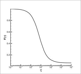
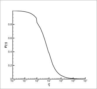
Figure 6: $F(\tau)$ as function of $\tau$ for solutions shown in Figure 5 (left) and Figure 1 (right)

5 The Wouthuysen-Field Coupling

We now estimate the time scale, $\tau_{\rm WF}$, of the onset of the W-F coupling. As mentioned in §4, in the first phase, $J(x,\tau)$ keeps the initial profile $\phi(x)$ of the photons from source $C$. In the second phase, the profile is no longer the initial one. A flat plateau (without recoil) or local Boltzmann distribution (with recoil) form the central part ($|x|\simeq 0$) due to the resonant scattering. The width of the flat plateau increases with the time $\tau$. Finally, in the third phase, the injection of Ly$\alpha$ photons from the source $C$ is balanced by the redshift, the height of the flat plateau or the local Boltzmann of $J(x,\tau)$ will stop increasing, and reach to a saturated value. The width of the flat or sloping plateau on the red side continuously increases.

As mentioned in Section 1, most works on the effect of the W-F coupling of 21 cm signal are based on the static solution of the Fokker-Planck approximation of eq.(10) (Chen & Miralda-Escude, 2004; Hirata, 2006; Furlanetto & Pritchard 2006; Chuzhoy & Shapiro 2006). Obviously, this solution corresponds to the third phase. Thus, the time scale of the W-F coupling is of the order of $\tau_{\rm III}$. Therefore, this approximation would be reasonable if the time scale of the formation and evolution of the 21 cm signal regions is larger than $\tau_{\rm III}$.

From Figures 4 and 6, one can see that the time scale of the onset of the third phase, $\tau_{\rm III}$, has to be of the order of $10^{2}$, and $10^{4}$ for $\gamma=$ $10^{-1}$, and $10^{-3}$ respectively, i. e. $\tau_{\rm III}$ is roughly equal to a few to ten of Gunn-Peterson optical depth. On the other hand, we can see from eq.(11) that $\gamma=$ $10^{-1}$, and $10^{-3}$ correspond to $f_{\rm HI}=$ $10^{-4}$, and $10^{-2}$ for the source at redshift $1+z=10$. Thus, for all cases, eq.(8) yields that the time scale $t_{\rm III}$ to be of the order of 1 Myr. The static solution of the Fokker-Planck equation would not be valuable for the 21 cm problem, if the time scale of the evolution of the 21 cm region is equal to or less than 1 Myr.

Actually the time-independent solution of eq. (10) would not be necessary for the 21 cm signal. The relative occupation of the two hyperfine-structure components of hydrogen ground state depends only upon the shape of the spectrum near the Ly-alpha frequency, regardless whether the solution is time-independent, or saturated. What we need for the W-F coupling is only the frequency distribution to show a local Boltzmann-like distribution $J(x,\tau)\propto\exp[-h(\nu-\nu_{0})/kT]$ around $\nu_{0}$, where $T$ is the kinetic temperature of hydrogen gas. The formation of the Boltzmann-like distribution is irrelevant to the time scale $\tau_{\rm III}$, but depends on the onset of the second phase of the $J(x,\tau)$ evolution.

Therefore, $\tau_{\rm WF}$ should be estimated by the time scale of the onset of the second phase, $\tau_{\rm II}$, not by $\tau_{\rm III}$. According to the property shown by Figure 6, $\tau_{\rm II}$ can be found by the formation of a flat plateau around the resonant frequency. For small $\gamma$, $\tau_{\rm II}$ is much less than $\tau_{\rm III}$. To show this point, we calculate the solution of eq.(10) with $\gamma=10^{-5}$ and $10^{-7}$ on static background. The results are given in Figure 7. It shows that that a small flat plateau has already formed at $\tau=100$. On the other hand, $\tau_{\rm III}$ will be as large as $\tau\simeq 10^{6}$ for $\gamma=10^{-5}$.

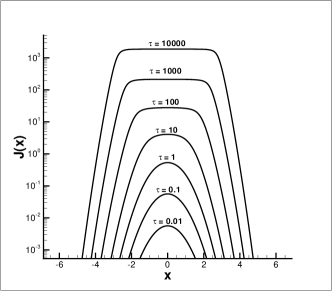
Figure 7: Solutions of $J(x,\tau)$ of eq.(10) with $\gamma=10^{-5}$ (left panel) and 10^-7 (right panel).

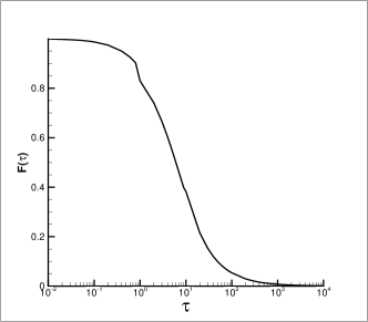
Figure 8: $F(\tau)$ as function of $\tau$ for solutions of $a=0$ and $\gamma=10^{-5}$ (left) and 10^-7(right).

In Figure 8, we show the function $F(\tau)$ for the parameters ($a=0$, $\gamma=10^{-5}$), and ($a=0$, $\gamma=10^{-7}$). It is interesting to observe that the two sets of $F(\tau)$ are almost identical. That is, the time scale $\tau_{\rm WF}$ is actually independent of the parameter $\gamma$. For both cases of the parameter $\gamma$, $\tau_{\rm WF}$ is equal to about a few of 10². In other words, a flat plateau with proper width can form with a few tens or hundreds of the mean free flight time of the resonant photons, regardless the expansion of the universe.

The reason of the $\gamma$-independence of $\tau_{\rm II}$ or $\tau_{\rm WF}$ can be directly seen from eq.(10). This equation describes two kinetic processes of approaching statistically steady state. The first is the resonant scattering, which leads to the formation of a flat plateau or local Boltzmann distribution around the resonant frequency. The second is the redshift of photons, which leads to a statistical equilibrium between the injected photons and redshifted photons. The steady state due to resonant scattering corresponds to the second phase, while the steady state due to redshift corresponds to the third phase. Similar to various statistical equilibrium or steady state maintained by collision or scattering, the steady state of resonant scattering can be realized via a few tens or hundreds of the resonant scattering. On the other hand, $\gamma$ is a ratio between the time scales of the resonant scattering and the expansion of the universe. Therefore, when $\gamma$ is much less than 1, the time scale of the formation of the flat plateau and local Boltzmann distribution are much shorter than the expansion of the universe. This point can also be seen with Figure 6, which shows that for $\gamma=10^{-5}$ and 10^-7 the evolutions of $J(x,\tau)$ actually are the same till $\tau=10^{4}$. In short, the W-F coupling will take place once a statistical equilibrium localized around the resonant frequency is realized.

6 Concluding remarks

To study the time scale of the W-F coupling, we need a better solution of the integro-differential equation of the resonant scattering of Ly$\alpha$ photons. Especially, we need to know the evolution of photon frequency distribution around the resonant scattering. That is, the algorithm should be able to handle the extremely flat distribution and its sharp boundary. These features can properly be captured by the WENO scheme, which has high order of accuracy and good convergence in capturing discontinuities as well as to be significantly superior over piecewise smooth solutions containing discontinuities. The WENO algorithm can be used for resonant scattering with and without the recoil of atoms. This algorithm is reliable as it passed all the tests.

The evolution of the photon distribution in the frequency space generally undergoes three phases. In the first phase, the profile of the photon distribution is similar to the initial one. In the second phase, an extremely flat plateau (without recoil) or Boltzmann distribution (with recoil) formed around the resonant frequency. The width and height of the flat plateau or local Boltzmann distribution increase with time. Finally, in the third phase, the photons injected from the source is balanced by the redshift of the expansion, and the evolution of the photon distribution is stable. The first phase is very short. The second phase will be onset after a few tens or hundreds of photons scattering by atoms. On the other hand, the onset of the third phase is mainly dependent on the Gunn-Peterson optical depth, which is large at early universe. Consequently, the onset of the third phase is much later than the second one.

Usually, the W-F coupling is described by time-independent solutions of the Fokker-Planck approximation of the integro-differential equation of the resonant scattering. With the WENO solutions, we show that the time-independent solutions would not be available for the 21 cm signal of the first generation stars, if the life time of the evolution of the 21 cm region is equal to or less than 1 Myr. However, the time scale of the onset of the W-F coupling actually is irrelevant with the time-independent solutions. The W-F coupling will take place once a statistical equilibrium is locally realized in the frequency space around the resonant frequency. This time scale is always a few tens or hundreds of the mean free flight time of the resonant photons, and is generally independent of the expansion of the universe when the Gunn-Peterson optical depth is large, or the Sobolev parameter is much less than 1. More detail results of the time-dependence o the W-F coupling is reported in Roy et al (2009).

Acknowledgments

This work is supported by the US NSF under the grants AST-0506734 and AST-0507340. We thank Dr. Jiren Liu for his help.

Appendix A Numerical integration: an $\mathcal{O}(N)$ algorithm

We need to numerically integrate $\displaystyle\int\mathcal{R}(x,x^{\prime})J(x^{\prime},t)dx^{\prime}$, denoted as

$$I(x)=\frac{1}{2}\int e^{2bx^{\prime}+b^{2}}{\rm erfc}(\max(|x+b|,|x^{\prime}+b|))J(x^{\prime},t)dx^{\prime},$$ (29)

with $\mathcal{R}(x,x^{\prime})$ as in eq.(7). To evaluate $I_{m}=I(x_{m})$, $\forall m=-N_{l},\cdots,N_{r}$, we apply the rectangular rule, which is spectrally accurate for smooth functions vanishing at boundaries,

$$I_{m} = \frac{1}{2}\int_{x_{left}}^{x_{right}}{\rm erfc}(\max(|x_{m}+b|,|x^{\prime}+b|))e^{2bx^{\prime}+b^{2}}J(x^{\prime},t)dx^{\prime}$$ (30)

$$\approx \frac{1}{2}\Delta x\sum_{i=-N_{l}}^{N_{r}}{\rm erfc}(\max(|x_{m}+b|,|x_{i}+b|))e^{2bx_{i}+b^{2}}J(x_{i},t).$$ (31)

Notice that this summation algorithm is very costly as it takes $\mathcal{O}(N)$ operations per $m$, therefore the total procedure has $\mathcal{O}(N^{2})$ operations overall. We use a grouping technique, described below, so that the overall computational cost can be reduced to $\mathcal{O}(N)$, without changing mathematically the algorithm and its accuracy.

The proposed scheme with order $N$ computational effort is the following. Let $N_{b}=floor(\frac{b}{\Delta x})$ and $N_{2b}=floor(\frac{2b}{\Delta x})$. The integration algorithm is designed for two cases: $m\geq-N_{b}$ and $m<-N_{b}$.

In the case of $m\geq-N_{b}$ or equivalently $x_{m}+b\geq 0$:

$$I_{m} = \frac{1}{2}\Delta x(\sum_{i=-N_{l}}^{-m-N_{2b}-1}{\rm erfc}(|x_{i}+b|)e^{2bx_{i}+b^{2}}J(x_{i},t)$$ (32)

$$+{\rm erfc}(|x_{m}+b|)\sum_{i=-m-N_{2b}}^{m}e^{2bx_{i}+b^{2}}J(x_{i},t)$$

$$+\sum_{i=m+1}^{N_{r}}{\rm erfc}(|x_{i}+b|)e^{2bx_{i}+b^{2}}J(x_{i},t))$$

$$\doteq \frac{1}{2}\Delta x(I_{1,m}+{\rm erfc}(|x_{m}+b|)I_{2,m}+I_{3,m})$$ (33)

1. Evaluate $I_{1,-N_{b}}$, $I_{2,-N_{b}}$ and $I_{3,-N_{b}}$ respectively as

   $$I_{1,-N_{b}} = \sum_{i=-N_{l}}^{N_{b}-N_{2b}-1}{\rm erfc}(|x_{i}+b|)e^{2bx_{i}+b^{2}}J(x_{i},t),$$ (34)

   $$I_{2,-N_{b}} = \sum_{i=N_{b}-N_{2b}}^{-N_{b}}e^{2bx_{i}+b^{2}}J(x_{i},t),$$ (35)

   $$I_{3,-N_{b}} = \sum_{i=-N_{b}+1}^{N_{r}}{\rm erfc}(|x_{i}+b|)e^{2bx_{i}+b^{2}}J(x_{i},t),$$ (36)

   which leads to $\mathcal{O}(N)$ cost.

2. DO $m=-N_{b}+1,N_{r}$ Evaluate $I_{2,m}$, $I_{3,m}$ respectively by

   $$I_{1,m}=I_{1,m-1}-{\rm erfc}(|x_{-m-N_{2b}}+b|)e^{2bx_{-m-N_{2b}}+b^{2}}J(x_{-m-N_{2b}},t)$$ (37)

   $$I_{2,m}=I_{2,m-1}+e^{2bx_{m}+b^{2}}J(x_{m},t)+e^{2bx_{-m-N_{2b}}+b^{2}}J(x_{-m-N_{2b}},t)$$ (38)

   $$I_{3,m}=I_{3,m-1}-{\rm erfc}(|x_{m}+b|)e^{2bx_{m}+b^{2}}J(x_{m},t)$$ (39)

   ENDDO

   To be consistent with the indeces, if $N_{l}-N_{2b}<N_{r}$ then, we will set $I_{1,m}=0$, for $m=N_{l}-N_{2b},N_{r}$. The algorithm leads to $\mathcal{O}(1)$ cost per $m$, therefore $\mathcal{O}(N)$ computation overall.

In the case of $m<-N_{b}$, or equivalently $x_{m}+b<0$:

$$I_{m} = \frac{1}{2}\Delta x(\sum_{i=-N_{l}}^{m-1}{\rm erfc}(|x_{i}+b|)e^{2bx_{i}+b^{2}}J(x_{i},t)$$ (40)

$$+{\rm erfc}(|x_{m}+b|)\sum_{i=m}^{-m-N_{2b}-1}e^{2bx_{i}+b^{2}}J(x_{i},t)$$

$$+\sum_{i=-m-N_{2b}}^{N_{r}}{\rm erfc}(|x_{i}+b|)e^{2bx_{i}+b^{2}}J(x_{i},t))$$

$$= \frac{1}{2}\Delta x(I_{1,m}+{\rm erfc}(|x_{m}+b|)I_{2,m}+I_{3,m})$$ (41)

1. Evaluate $I_{1,-N_{b}-1}$, $I_{2,-N_{b}-1}$ and $I_{3,-N_{b}-1}$ as

   $$I_{1,-N_{b}-1} = \sum_{i=-N_{l}}^{-N_{b}-2}{\rm erfc}(|x_{i}+b|)e^{2bx_{i}+b^{2}}J(x_{i},t),$$ (42)

   $$I_{2,-N_{b}-1} = \sum^{N_{b}-N_{2b}}_{i=-N_{b}-1}e^{2bx_{i}+b^{2}}J(x_{i},t),$$ (43)

   $$I_{3,-N_{b}-1} = \sum_{i=N_{b}+1-N_{2b}}^{N_{r}}{\rm erfc}(|x_{i}+b|)e^{2bx_{i}+b^{2}}J(x_{i},t),$$ (44)

   which leads to $\mathcal{O}(N)$ cost.

2. DO $m=-N_{b}-2,-N_{l}$

   Evaluate $I_{1,m}$, $I_{2,m}$, $I_{3,m}$ respectively by

   $$I_{1,m}=I_{1,m+1}-{\rm erfc}(|x_{m}+b|)e^{2bx_{m}+b^{2}}J(x_{m},t)$$ (45)

   $$I_{2,m}=I_{2,m+1}+e^{2bx_{m}+b^{2}}J(x_{m},t)+e^{2bx_{-m-N_{2b}-1}+b^{2}}J(x_{-m-N_{2b}-1},t)$$ (46)

   $$I_{3,m}=I_{3,m+1}-{\rm erfc}(|x_{-m-N_{2b}-1}+b|)e^{2bx_{-m-N_{2b}-1}+b^{2}}J(x_{-m-N_{2b}-1},t)$$ (47)

   ENDDO

   To be consistent with the indeces, if $N_{l}-N_{2b}>N_{r}$, we will set $I_{3,m}=0$, for $m=-N_{2b}-N_{r}-1,-N_{l}$. Again, the algorithm leads to $\mathcal{O}(1)$ cost per $m$, therefore $\mathcal{O}(N)$ computation overall.

References

- (1) Basko, M.M. 1981, Astrophysics, 17, 69
- (2) Carrillo, J.A., Gamba, I.M., Majorana, A. & Shu, C.-W. 2003, J. Comput. Phys., 184, 498
- (3) Carrillo, J.A., Gamba, I.M., Majorana, A. & Shu, C.-W. 2006, J. Comput. Phys., 214, 55
- (4) Cen, R. 2006, ApJ, 648, 47
- (5) Chen, X. & Miralda-Escude, J. 2004, ApJ, 602, 1.
- (6) Chuzhoy, L., Alvarez, M. A., & Shapiro, P. R. 2006, ApJ, 648, L1
- (7) Chuzhoy, L. & Shapiro, P.R. 2006, ApJ, 655, 843
- (8) Field, G.B., 1958, Proc. IRE, 46, 240
- (9) Field, G.B. 1959, ApJ, 129, 551.
- (10) Furlanetto, S.R. & Pritchard, J.R. 2006, MNRAS, 372, 1093
- (11) Henyey, L.G. 1941, Proc. Nat. Acad. Sci. 26, 50
- (12) Hirata, C.M. 2006, MNRAS, 367, 259
- (13) Hummer, D.G. 1962, MNRAS, 130, 295
- (14) Hummer, D.G. 1969, MNRAS, 145, 95
- (15) Hummer, D.G. & Rybicki, G.B. 1992, ApJ, 387, 248.
- (16) Jiang, G. & Shu, C.W. 1996, J. Comput. Phys., 126, 202
- (17) Liu, J.R., Qiu, J.M., Feng, L.L., Shu, C.W. and Fang, L.Z. 2007, ApJ, 663, 1
- (18) Meiksin, A. 2006, MNRAS, 370, 2025
- (19) Qiu, J.M., Feng, L.L., Shu, C.W. & Fang, L.Z. 2006, New Astronomy, 12, 1
- (20) Qiu, J.M., Feng, L.L., Shu, C.W. & Fang, L.Z. 2007, New Astronomy, 12, 398
- (21) Qiu, J.M., Shu, C.W., Liu, J.R. & Fang, L.Z. 2008, New Astronomy, 13, 1
- (22) Roy, I., Xu, W., Qiu, J.M., Shu, C.W. & Fang, L.Z. 2009, arXiv:0812.4104, Astrophys. J. in press
- (23) Rybicki G.B. & Dell’Antonio, I.P. 1994, ApJ, 427, 603
- (24) Shen, J., Shu, C.W. & Zhang, M. 2007, J. Sci Comput, 33, 279
- (25) Shu, C.-W., 2003, Int. J. Comp. Fluid Dyn., 17, 107
- (26) Shu, C.-W. & Osher, S., 1988, J. Comp. Phys., 77, 439
- (27) Wouthuysen, S. A. 1952, AJ, 57, 31