Abstract

Several integrate-to-threshold models with differing temporal integration mechanisms have been proposed to describe the accumulation of sensory evidence to a prescribed level prior to motor response in perceptual decision-making tasks. An experiment and simulation studies have shown that the introduction of time-varying perturbations during integration may distinguish among some of these models. Here, we present computer simulations and mathematical proofs that provide more rigorous comparisons among one-dimensional stochastic differential equation models. Using two perturbation protocols and focusing on the resulting changes in the means and standard deviations of decision times, we show that, for high signal-to-noise ratios, drift-diffusion models with constant and time-varying drift rates can be distinguished from Ornstein-Uhlenbeck processes, but not necessarily from each other. The protocols can also distinguish stable from unstable Ornstein-Uhlenbeck processes, and we show that a nonlinear integrator can be distinguished from these linear models by changes in standard deviations. The protocols can be implemented in behavioral experiments.

1 Introduction

Reaction time tasks have long been used to study human decision making (Luce,, 1986). One paradigm requires subjects to detect or discriminate sensory signals by making a voluntary motor response. Response time distributions obtained in such perceptual-motor tasks allow inference of cognitive information processing (Posner,, 1978). With the advent of methods for recording neural activity in awake behaving animals, such tasks have been adopted by neurophysiologists, especially in studies on monkeys (Schall,, 2003; Gold and Shadlen,, 2007), and neuronal firing rates in several brain areas have been shown to correlate with motor responses. The lateral intraparietal area, frontal eye fields, and superior colliculus (Gold and Shadlen,, 2007) all exhibit activities that ramp up over time toward a fixed level before a decision is signaled (e.g. by a saccadic eye movement in the direction of the recorded response field) (Hanes and Schall,, 1996; Roitman and Shadlen,, 2002; Churchland et al.,, 2008). The slopes of the ramps not only correlate with task difficulty (the harder the task, the lower the slope), but also with response time (higher slopes precede faster responses). These areas may therefore provide neural substrates for integrating sensory information toward a decision criterion before a perceptual decision is made.

Various integrate-to-threshold models have been proposed to describe both response times and neurobiological mechanisms (Smith and Ratcliff,, 2004), including drift-diffusion models (Ratcliff,, 1978; Mazurek et al.,, 2003; Smith and Ratcliff,, 2004; Ditterich, 2006a, ; Simen et al.,, 2006; Ratcliff and McKoon,, 2008) and attractor neural networks with mutual inhibition (Brown and Holmes,, 2001; Usher and McClelland,, 2001; Wang,, 2002; Wong and Wang,, 2006; Lo and Wang,, 2006). All share a common mechanism: accumulation or integration of sensory inputs toward a prescribed threshold, the first crossing of which determines the decision and response time. These models may nonetheless be distinguished by the details of the integration process: drift-diffusion models typically accumulate evidence at a constant rate like a biased random walk, while attractor networks have unstable or stable steady-states that can, respectively, accelerate or decelerate the integration process (Usher and McClelland,, 2001; Wong and Wang,, 2006).

Often only behavioral data are collected for human subjects, and fits based on response times and choice accuracies are sometimes unable to distinguish among competing models (Ratcliff et al.,, 1999; Ratcliff,, 2006). Moreover, while cellular recordings in awake behaving animals offer direct insights into the integration process, fitting of both behavioral and neural data may still not suffice, especially when models incorporate multiple features and depend on multiple parameters. For example, a drift-diffusion model with a time-dependent ‘urgency’ signal (Ditterich, 2006a, ; Churchland et al.,, 2008) may be difficult to separate from a recurrent network model with strong self-excitation (Wang,, 2002; Wong and Wang,, 2006). Thus far, few principled attempts have been made to tease apart different integration mechanisms.

Subthreshold electrical microstimulation of neural activities in behaving animals may provide more conclusive tests (Cohen and Newsome,, 2004). In Ditterch et al., (2003), microstimulation of sensory neurons was shown to affect the speed of the decision. More interestingly, in Hanks et al., (2006), stimulation of cells with choice targets in the recorded neuronal response fields speeded decisions, but also reduced decision speeds when choice target directions were opposite to the recorded response fields, thus providing evidence of mutual inhibition. Perturbations need not be invasive, and so can be used in human studies: e.g., Huk and Shadlen, (2005) employed a brief motion pulse in the background of the primary visual stimulus; although it neither determined the choice nor influenced rewards, the pulse had a significant effect on response times.

Earlier modeling efforts (Huk and Shadlen,, 2005; Wong et al.,, 2007; Wong and Huk,, 2008) have addressed the data of Huk and Shadlen, (2005), but they employed many parameters and direct comparisons were not made between models. Here, we conduct a more rigorous study using simpler models, and seek more objective comparisons among them. We approximate four neural firing rate models as linear, scalar, stochastic differential equations (SDE), and we ask how their predicted response times are affected by short piecewise-constant perturbations with varying onset times and amplitudes. By comparing changes in means and standard deviations of response times, we demonstrate that the perturbations suffice to distinguish among the models. Finally, we show that a nonlinear integrator model, qualitatively similar to that of Wong and Wang, (2006), behaves much like one of the linear models.

2 Methods

2.1 Reduction to one-dimensional linear integrate-to-threshold models

Two-alternative forced-choice decision processes can, in essence, be modeled by two populations of excitatory neurons each endowed with self-excitatory connections and mutual inhibition via a shared inhibitory population. Each of the three populations can then be represented in a coarse-grained firing rate model by a single unit whose state describes the population-averaged activity $r_{j}(t)$ of the corresponding neuronal pool (Wilson and Cowan,, 1972, 1973). Here we review the further reduction of a firing rate model, under suitable hypotheses, to a one-dimensional dynamical system. For additional details, see Brown et al., (2005); Bogacz et al., (2006).

Consider first the deterministic equations describing the firing rates of two excitatory ($E$) populations and a common inhibitory ($I$) population:

$$\tau_{E}\frac{dr_{1}}{dt} = -r_{1}+F_{E}(r_{1},r_{2},r_{I},I_{1}),$$

$$\tau_{E}\frac{dr_{2}}{dt} = -r_{2}+F_{E}(r_{2},r_{1},r_{I},I_{2}),$$ (1)

$$\tau_{I}\frac{dr_{I}}{dt} = -r_{I}+F_{I}(r_{1},r_{2}).$$

Here $\tau_{E}$ and $\tau_{I}$ are the synaptic time constants for the $E$ and $I$ units, and $r_{1}$, $r_{2}$ and $r_{I}$ are respectively the activity of neural units $1$, $2$ and $I$. The excitatory populations $1$ and $2$ are selective to stimuli $1$ and $2$, respectively. $F_{E}$ and $F_{I}$ are their input-output functions, and the overall input to each unit, with $i=E$ or $I$, is $I_{i}=I_{recurrent,i}+I_{stimulus,i}$. The decision time is the first passage time from stimulus onset to the first of $r_{1}$ or $r_{2}$ reaching a prescribed decision threshold, which thereby signals choice $1$ or $2$. Since non-decision latencies (e.g. signal transduction and motor preparation) are usually assumed to be independent of stimulus strength $I_{stimulus}$, we shall model the response time as the decision time plus a constant latency. Henceforth we use the phrases ‘decision time’, ‘reaction time’ and ‘response time’ interchangeably.

If the decision dynamics passes near a saddle point and moves along its unstable manifold (Brown and Holmes,, 2001; Bogacz et al.,, 2006), the functions $F_{E},\,F_{I}$ may be linearized such that Eq. 1 simplifies to:

$$\tau_{E}\frac{dr_{1}}{dt} = -r_{1}+(\alpha r_{1}-\beta r_{I}+I_{1}+I_{0,E}),$$

$$\tau_{E}\frac{dr_{2}}{dt} = -r_{2}+(\alpha r_{2}-\beta r_{I}+I_{2}+I_{0,E}),$$ (2)

$$\tau_{I}\frac{dr_{I}}{dt} = -r_{I}+(\gamma r_{1}+\gamma r_{2}+I_{0,I}).$$

Here $\alpha,\beta,\gamma$ are the recurrent synaptic coupling strengths for self-excitation, inhibitory-to-excitatory, and excitatory-to-inhibitory connections, and $I_{0,E}$ ($I_{0,I}$) is the constant background input to all the excitatory (inhibitory) cells from outside the local circuit. Unlike Wang, (2002), we exclude excitatory connections between $r_{1}$ and $r_{2}$ and self-inhibitory connections, retaining only essential features. If $\tau_{I}\ll\tau_{E}$, we can further assume that the relatively fast dynamics of $r_{I}$ equilibrates rapidly, such that $r_{I}\approx\gamma(r_{1}+r_{2})+I_{0,I}$, and Eq. 2 becomes

$$\tau_{E}\frac{dr_{1}}{dt} = -r_{1}+(\alpha-\beta\gamma)r_{1}-\beta\gamma r_{2}+I_{1}+(I_{0,E}-\beta I_{0,I}),$$ (3)

$$\tau_{E}\frac{dr_{2}}{dt} = -r_{2}+(\alpha-\beta\gamma)r_{2}-\beta\gamma r_{1}+I_{2}+(I_{0,E}-\beta I_{0,I}).$$ (4)

Defining a new variable $X\equiv r_{1}-r_{2}$ and subtracting Eq. 4 from 3, we obtain

$$\frac{dX}{dt}=kX+(I_{1}(t)-I_{2}(t))/\tau_{E},$$

where $k\equiv(\alpha-1)/\tau_{E}$ contains the excitatory coupling strength and leak, and $(I_{1}-I_{2})/\tau_{E}$ is proportional to the difference in inputs. The background inputs $I_{0,E}$ and $I_{0,I}$ and coupling strengths $\beta$ and $\gamma$ cancel out.

Generalizing the inputs $I_{1}$, $I_{2}$ to be time-varying and including additive noise, the reduced dynamics is described by a one-dimensional SDE of the form

$$dX_{t}=b(X_{t},t)dt+\sigma dW_{t},$$ (5)

where $b(X_{t},t)\equiv kX_{t}+(I_{1}(t)-I_{2}(t))/\tau_{E}$ and $\sigma$ is the standard deviation of the noise, which is assumed to be a Wiener process with increments $dW_{t}$ drawn from a normal distribution with zero mean and unit variance. Eq. 5 provides a general description for noisy accumulator models, as illustrated schematically in Fig. 1A.

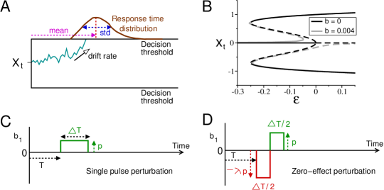
Figure 1: One-dimensional integrate-to-threshold models and perturbation protocols. A: a general model for a two-alternative forced-choice reaction time task. Here the noisy state $X_{t}$, which quantifies the difference in firing rates between two competing excitatory cell populations, reaches the upper decision threshold in a sample trial, and choice is correct since threshold is in same direction as drift rate. Multiple sampling provides the response time distribution. B: the SPB model with unbiased input exhibits a subcritical pitchfork bifurcation at $\varepsilon=0$. Black curves show branches of stable (solid) and unstable (dashed) fixed points in the noiseless limit; branches for biased input shown in gray. C: a short pulse can be repeated over a range of onset times $T$ after primary stimulus onset at $t=0$ to test effects on decision times. D: a pulse-antipulse perturbation whose leading pulse amplitude (red) can be adjusted to determine when decision times are unaffected by the combined pulse, yielding a zero-effect perturbation (ZEP). See text for further details.

2.2 Linear integrate-to-threshold models

We are now in a position to introduce four linear instances of Eq. 5. When $k<0$ (e.g. self-excitation $\alpha$ is relatively weak), we have a classical Ornstein-Uhlenbeck (OU) process (Uhlenbeck and Ornstein,, 1930; Wang and Uhlenbeck,, 1945). If the decision threshold does not intervene, solutions eventually decelerate and approach a stable steady-state $X_{steady-state}=(I_{1}(t)-I_{2}(t))/(|k|\tau_{E})$. We denote this stable OU process SOU; in contrast, if $k>0$ (stronger self-excitation), sample paths accelerate away from a fixed point in an unstable OU process, denoted UOU. SOU and UOU provide reduced descriptions of the leaky competing accumulator of Usher and McClelland, (2001) that respectively produce recency and primacy effects.

In the special case of $\alpha=1$ (i.e. $k=0$) and constant stimuli $I_{1}$, $I_{2}$, Eq. 5 becomes a pure drift-diffusion (CD) equation (Ratcliff,, 1978)

$$dX_{t}=b_{0}dt+\sigma dW_{t},$$ (6)

in which the constant drift rate $b=b_{0}\equiv(I_{1}-I_{2})/\tau_{E}$ is proportional to the difference in stimuli. This CD model is similar to, but differs in detail from, the balance between leakage and inhibition in Bogacz et al., (2006).)

In some variants of the CD model, drift rates can vary with time. This could be due to dynamic stimuli, to some form of ‘urgency’ induced by the task design (Ditterich, 2006a, ; Ditterich, 2006b, ; Churchland et al.,, 2008), to fluctuating attention (Smith et al.,, 2004) or to other ‘top-down’ effects (Liu et al.,, 2008). This time-dependent (TD) diffusion model is described by:

$$dX_{t}=b(t)dt+\sigma dW_{t}.$$ (7)

We focus on the simple case $b(t)=b_{0}t$, since similar results obtain for other functions of time, but in Appendix B, we treat a modified TD model with time-varying perturbation amplitude.

2.3 A nonlinear integrate-to-threshold model

The final model to be considered is qualitatively similar to that of Wang, (2002); Wong and Wang, (2006). It captures stochastic dynamics in the neighborhood of a subcritical pitchfork bifurcation (Guckenheimer and Holmes,, 1983; Brown and Holmes,, 2001; Strogatz,, 2001) that occurs as the stimulus input level is varied (Roxin and Ledberg,, 2008; Wong and Wang,, 2006):

$$\tau_{X}dX_{t}=[\varepsilon X_{t}+X_{t}^{3}-X_{t}^{5}+b(t)]dt+\sigma dW_{t}.$$ (8)

Here $b(t)\equiv b_{0}$ (constant) and $\varepsilon$ represent the biased and non-biased stimulus inputs respectively (Fig. 1B). $\tau_{X}$ controls the overall temporal dynamics. Eq. 8 may be derived by normal form theory (Guckenheimer and Holmes,, 1983; Roxin and Ledberg,, 2008): see Fig. 1B for an illustration of the branches of stable and unstable fixed points in the noise-free limit. If $|\varepsilon|$ and $|b|$ are sufficiently small, this model without the $X_{t}^{5}$ term approaches that of Wang, (2002); Wong and Wang, (2006); Roxin and Ledberg, (2008). We include $-X_{t}^{5}$ to prevent unrealistic runaway activity, and, for simplicity, first assume a symmetrical system with $b_{0}=0$, and then consider biased stimuli $|b_{0}|>0$. This model is denoted SPB.

2.4 Perturbation protocols

2.4.1 Single pulse perturbation with varying onset time

We consider additive perturbations $b_{1}(t)$, under which Eq. 5 becomes $dX_{t}=[b(X_{t},t)+b_{1}(t)]dt+\sigma dW_{t}$, where $b_{1}(t)$ is applied from time $T$ to $T+\Delta T$ and $b_{1}(t)\equiv 0$ otherwise. We employ two piecewise-constant forms, the first being the step function used by Huk and Shadlen, (2005):

$$b_{1}(t)=\left\{\begin{array}[]{ll }0,&t\leq T,\\ p,&T<t\leq T+\Delta T,\\ 0,&t>T+\Delta T,\end{array}\right.$$ (9)

in which the amplitude $p$ can be positive or negative, assisting or opposing the unperturbed drift rate $b_{0}$ due to the ‘primary’ stimulus. We fix the duration $\Delta T$ at $10\%$ of the unperturbed mean first passage time $\tau_{0}/10$, apply $b_{1}$ at different onset times $T$ and ask how the mean and standard deviation of the decision time change.

2.4.2 Zero-effect pulse-antipulse perturbation

The second protocol uses a double pulse of the form

$$b_{1}(t)=\left\{\begin{array}[]{ll }0,&t\leq T,\\ -\lambda p,&T<t\leq T+\Delta T/2,\\ p,&T+\Delta T/2\leq t<T+\Delta T,\\ 0,&t>T+\Delta T,\end{array}\right.$$ (10)

where $\lambda$ is the relative height of the first pulse to the second. The second opposite-signed pulse attempts to reduce or cancel the expected change due to the first, and if the overall perturbation $b_{1}$ leaves the mean first passage time unchanged, we call it a zero-effect perturbation or ZEP. This protocol, a variant of the paired pulse suggested in Wong et al., (2007), is only applied early in the integration process to avoid interference from the decision threshold. We shall seek critical values of $\lambda$ for which ZEPs occur for each model. Figs. 1C and D illustrate both protocols.

2.5 Simulations and parameter values

Except for the SPB model, we first consider integration to a single decision threshold in the direction of the drift. This reduces the number of parameters, simplifies mathematical analyses, and helps isolate key effects. It applies to easy tasks in which drift rates are (relatively) high and errors rare. We subsequently relax this condition in our simulations. For the SPB model we first set $I_{1}=I_{2}$, corresponding to difficult tasks and high error rates, and employ two thresholds. We then consider $I_{1}\neq I_{2}$ and a single threshold, representing easy tasks.

Signal-to-noise ratios were chosen such that the variance in first passage (decision) times is significant, but not so great that an unreasonably large number of trials is needed to average out the noise, and we selected perturbation amplitudes, durations and onset times such that both protocols cause small but significant effects (e.g. maximum changes of $\sim 10\%$ in mean decision times). In particular, durations were an order of magnitude smaller than mean decision times $\tau_{0}$, as in Huk and Shadlen, (2005). For the first protocol, onset times $T$ were varied from stimulus onset at $t=0$ until there were no significant effects on mean decision time. In the second protocol we require $T\ll\tau_{0}$. We set $X_{0}=0$ at $t=0$ to represent unbiased initial conditions, and the remaining parameters are chosen to ensure ‘realistic’ behavior (e.g. the stable fixed point is above threshold for SOU; the unstable fixed point is below $X_{0}=0$ for UOU). Table 1 lists parameter values.

Model	$b(X_{t},t)$	Parameters	$\zeta$	$\Delta T$	$p$
CD	$b_{0}+b_{1}$	$b_{0}=5,\sigma=2.449$	$20$	$0.4$	$5$
TD	$b_{0}t+b_{1}$	$b_{0}=4,\sigma=2.828$	$20$	$0.1$	$4$
SOU	$kX_{t}+b_{0}$	$k=-1,b_{0}=8$,	$7$	$0.4$	$2$
	$+b_{1}$	$\sigma=1.414$
UOU	$kX_{t}+b_{0}$	$k=0.2,b_{0}=5$,	$20$	$1$	$2$
	$+b_{1}$	$\sigma=1.414$
SPB	$\varepsilon X_{t}+X_{t}^{3}$	$\varepsilon=-0.3,0.05,b_{0}=0$	$\pm 0.75$	$5$	$0.005$
	$-X_{t}^{5}+b_{0}$	or $0.004$, $\sigma=0.01$,			or $0.0008$
	$+b_{1}$	$\tau_{X}=20$			($b_{0}=0.004$)

Table 1: Parameters used in simulations. Drift-diffusion model with constant drift rate (CD), and with time-varying drift rate (TD); SOU (UOU) stable (unstable) Ornstein-Uhlenbeck processes; SPB: nonlinear model. See Eqs. 5-8 and protocols 9 and 10 for details. Here $\zeta$ is the distance from starting point $X=0$ to decision threshold, and for SPB $\varepsilon=-0.3$ before stimulus appears at $t=0$ and $\varepsilon=0.05$ for $t\geq 0$. Perturbation durations $\Delta T$ and amplitudes $p$ are values used in the first perturbation protocol. Parameters for the linear models with smaller signal-to-noise ratios are specified in Section 3.3.

We use a forward Euler-Maruyama scheme (Higham,, 2001), integrating a sample path until it hits the prescribed decision threshold and recording the corresponding first passage time, at which the trial ends and the next begins. After collecting an appropriately large ensemble, we extract the first and second moments of the first passage time from the samples. The simulation is run once for each one of the different perturbations. For the models CD, TD, SOU and UOU, the step size is $10^{-3}$ of a time unit and the sample size is $N=10^{6}$, so that errors in the moments are of order $1/\sqrt{N}\approx 10^{-3}$. Since changes in moments due to the perturbations are of order $10^{-2}$, these choices of time step and sample size reliably capture the effects of perturbation. The mean exit time for the unperturbed SPB model is $\sim 80$, so that a time step of $0.01$ and a sample size is $10^{6}$ suffices. We ran noisy simulations of this model with $\varepsilon=-0.3$ for $t<0$ to represent pre-stimulus activity, and then switched to $\varepsilon=0.05$ for $t\geq 0$ so that $X=0$ undergoes a pitchfork bifurcation and becomes unstable, thus forcing a choice (see Fig. 1B. Magnitudes of $\varepsilon$ and $\sigma$ for SPB are much smaller than the corresponding $b_{0}$ and $\sigma$ for the linear models because the $+X_{t}^{3}$ term accelerates solutions toward the thresholds).

The parameters are not independent, and their number can be reduced by one in all models by dividing Eq. 5 by $b_{0}$, and rescaling $\sigma\rightarrow\sigma/b_{0}$, $p\rightarrow p/b_{0}$, $\zeta\rightarrow\zeta/b_{0}$, $k\rightarrow k/b_{0}$ and the dynamical variable $X_{t}\rightarrow X_{t}/b_{0}$. The resulting CD and TD models are described by $2$ parameters while the SOU and UOU models require 3 and the SPB model $4$. Two additional parameters describe the amplitude $p$ and duration $\Delta T$ of the perturbation.

We focus on qualitative patterns of changes in response times and, to make unbiased comparisons, we adopt a dimensionless measure of the changes in means and standard deviations by normalizing the relative changes with respect to their unperturbed values.

3 Results

3.1 Single pulse perturbations of linear models

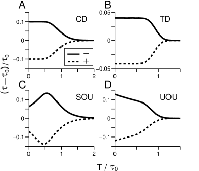
Figure 2: Changes in mean decision times under single pulse perturbations with varying onset times superimposed on positive drift rates for linear integrators CD, TD, SOU, and UOU (panels A-D). Vertical axes: normalized changes in mean first passage times $(\tau-\tau_{0})/\tau_{0}$; horizontal axes: normalized perturbation onset times $T/\tau_{0}$. Changes due to negative pulses shown solid ($-$); changes due to positive pulses dashed ($+$). CD and TD show near-constant changes for $T/\tau_{0}\leq 0.5$ that are substantially greater for CD (note vertical scale on panel B), SOU exhibits a maximum at $T/\tau_{0}\approx 0.5$ (“optimal” perturbation), and UOU shows monotonic decrease. Effects decrease in all cases as $T$ approaches and passes $\tau_{0}$ due to thresholding (see text).

Using a single pulse perturbation with varying onset time $T$, we estimated changes in mean decision time for the four linear integrate-to-threshold models as described above, obtaining the results shown in Fig. 2. Imposed early during the integration process, a brief pulse in the same (opposite) direction as the drift rate significantly decreases (increases) mean decision times in all four models, as shown by the dashed (solid) curves. These effects fade as $T$ increases due to a thresholding effect: for later perturbations, more trials have already crossed threshold, and so there are relatively fewer trials that are perturbed than unperturbed. Thus, when averaging over all trials, the influence of perturbations is progressively reduced. Note that unlike the work of Huk and Shadlen, (2005); Wong et al., (2007), trials that have crossed threshold before and during perturbation are not excluded in the averaging process. This helps to reduce noise in the data, especially with late perturbation onset times.

In Appendix A, we prove that this basic pattern – positive pulses advance mean decision times and negative pulses retard them – must hold provided that the perturbation occurs sufficiently early. The proof applies to a broad class of nonlinear systems including the SPB model of Eq. 8, provided that $\varepsilon>0$ and thresholds lie inside the region in which drift magnitude increases with $X$ (i.e., well below the activation levels of the stable fixed points).

Note that the drift-diffusion models (CD, TD) and the OU models (SOU, UOU) respond distinctly to early perturbations: the former exhibiting almost constant changes in mean decision times (panels A and B), and the latter respectively showing increasing and decreasing effects (panels C and D). Moreover, due to thresholding, SOU is alone in having an onset time for which the perturbative effect is maximized.

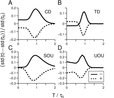
Figure 3: Changes in standard deviations of decision times under single pulse perturbations with varying onset times. All cases exhibit a maximum in normalized standard deviation (std$(\tau)-$std$(\tau_{0}))/$std$(\tau_{0})$, but only UOU has a (shallow) minimum. Effects of early pulses on all four integrators are distinct, as described in text. Format and conventions are as in Fig. 2.

We next investigate how standard deviations are affected by perturbation onset time: see Fig 3. Richer patterns arise than those of Fig. 2. Both CD and TD exhibit similar near-constant changes for early onsets, but the directions of changes for TD are opposite to those for CD, and the curves cross before reaching maxima. Standard deviations for SOU have a similar pattern to its mean, but UOU exhibits initial decreases followed by increases to a peak, unlike its mean. Optimal onset times exist for which the four standard deviations are maximally affected, and all four cases show distinct patterns.

In the TD model considered above we assumed that the perturbation is not affected by the time-dependent gain $b(t)$. This may not hold if the perturbation enters via the same sensory pathway as the stimuli. In Appendix B we consider a case in which perturbation and drift are affected in the same way. We show that this modified TD model differs qualitatively only for early perturbation onset, for which it yields reduced effects.

3.2 Zero-effect perturbations of linear models

We now consider the zero-effect protocol of Eq. 10, appealing to the fact that, in the noise-free case, the first passage time is a monotone function of the ratio $\lambda$ of the amplitudes of the opposing pulses. The critical $\lambda=\lambda^{*}$ that determines a ZEP is therefore given by the unique zero of

$$\tau(\lambda)=\tau_{0},$$ (11)

where $\tau(\lambda)$ describes the functional dependence of passage time on $\lambda$. Mean first passage times appear to remain monotone with respect to $\lambda$ when noise is included. Asymptotic methods can be used to approximate passage time moments for small perturbations (Lindner,, 2004), but the lack of compact formulae for passage time distributions (PDFs) in most cases, including OU processes, and the need for double integrations (Lindner,, 2004) makes this approach generally intractable.

However, ZEPs may be analytically approximated for early onset times $T$ with $T^{\prime}:=T+\Delta T\ll\tau_{0}$, such that the probability of threshold crossing prior to $T^{\prime}$ is negligible. In this case a sufficient condition is that the PDFs of the perturbed and unperturbed processes are identical at $T^{\prime}$, since for $t>T^{\prime}$, both processes are governed by the same drift and noise. They are therefore indistinguishable in the limit $T,\Delta T\rightarrow 0$. Before deriving explicit expressions for $\lambda^{*}$ under this assumption we present the results of numerical simulations with an intuitive explanation.

Since the unperturbed SDE (5) is independent of the current state $X_{t}$ in the CD and TD cases, we expect that antisymmetric pulses with $\lambda^{*}=1$, in which the pulses precisely cancel, will produce ZEPs. In contrast, responses to inputs decay with time for SOU, implying that the first pulse must be larger than the second for their net effect to cancel at perturbation offset $t=T^{\prime}$ ($\lambda^{*}>1$). For UOU the reverse should hold ($\lambda^{*}<1$). Fig. 4 confirms that this is the case. Table 2 lists the parameters used in the simulations; note that the early onset time conditions are only weakly satisfied ($T^{\prime}$ ranges from $25-40\%$ of $\tau_{0}$).

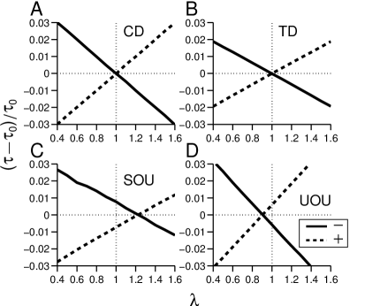
Figure 4: Zero-effect perturbations of linear integrate-to-threshold models CD, TD, SOU, UOU (panels A-D). Vertical axes: normalized change in mean first passage times $(\tau-\tau_{0})/\tau_{0}$; horizontal axes: relative amplitude $\lambda$ of first pulse compared to second. Zeroes of solid lines ($-$, positive pulse followed by negative pulse, $p<0$) and dashed lines ($+$, negative pulse followed by positive pulse, $p>0$) identify ZEPs at $\lambda^{*}\approx 0.9987,1.0039$ (CD); $0.9952,1.0004$ (TD); $1.2271,1.2230$ (SOU) and $0.9066,0.9034$ (UOU).

Model	$\tau_{0}$	std($\tau_{0}$)	$T$	$\Delta T$	$p$	$\lambda^{*}$ (thy.)	$\lambda^{*}$ (sim.)
CD	$4.005$	$0.960$	$0.5$	$0.5$	$5$	$1$	$1.0013$
TD	$3.145$	$0.420$	$0.5$	$0.5$	$5$	$1$	$0.9978$
SOU	$1.831$	$0.374$	$0.1$	$0.4$	$2$	$1.2214$	$1.2251$
UOU	$2.954$	$0.142$	$0.2$	$1.0$	$2$	$0.9048$	$0.9050$

Table 2: Parameters used in ZEP simulations. $\tau_{0}$ and std($\tau_{0}$) are the first and second moments of the passage time without perturbation, $T$ and $\Delta T$ are the onset time and total duration of the perturbation; $p$ is the amplitude of the second pulse and $\lambda^{*}$ (thy.) and $\lambda^{*}$ (sim.) are the ZEP pulse ratios predicted by the theory and obtained by averaging $p<0$ and $p>0$ results of Fig. 4.

To derive explicit approximations for $\lambda^{*}$, we use a comparison method similar to that of Appendix A. Let $X_{t}$ denote the unperturbed process and $Z_{t}$ the perturbed process. If $X_{0}=Z_{0}$ at $t=0$, then $X_{T}=Z_{T}$ at the onset time $T$. When the perturbation ends at $t=T^{\prime}$ the solution of the unperturbed SDE of Eq. 5 with constant drift rate $b_{0}$ is

$$X_{T^{\prime}}=(X_{T}+b_{0}/k)e^{k\Delta T}-b_{0}/k+\sigma\int_{T}^{T+\Delta T}e^{k(T^{\prime}-s)}dW_{s},$$ (12)

while the perturbed system satisfies

$$Z_{T^{\prime}}=(X_{T}+b_{0}/k)e^{k\Delta T}-b_{0}/k+\int_{T}^{T+\Delta T}e^{k(\Delta T-s)}b_{1}(s)ds+\sigma\int_{T}^{T+\Delta T}e^{k(T^{\prime}-s)}dW_{s}.$$ (13)

These expressions well approximate the true activity levels for models CD, SOU and UOU with absorbing thresholds only when both processes have low probability of hitting the threshold during the interval $[0,T^{\prime}]$, but this condition holds for $T^{\prime}/\tau_{0}\ll 1$, since the integrated drift term is almost zero at early times. Eqs. 12 and 13 differ in the term $e^{k\Delta T}\int_{0}^{\Delta T}e^{-kt}b_{1}(t)dt$, which enters $Z_{T^{\prime}}$ due to the action of the perturbation $b_{1}$ during the interval $[T,T^{\prime}]$. The ZEP condition for arbitrary perturbations is therefore

$$\int_{T}^{T+\Delta T}e^{-kt}b_{1}(t)dt=0,$$ (14)

which for the piecewise constant pulses of Eq. 10 implies that:

$$\lambda^{*}=\frac{e^{-k\Delta T/2}-e^{-k\Delta T}}{1-e^{-k\Delta T/2}}=e^{-k\Delta T/2}.$$ (15)

Hence for $k>0$ (UOU), $\lambda^{*}<1$, while for $k<0$ (SOU), $\lambda^{*}>1$. In the special case of CD, $k=0$ and $\lambda^{*}=1$.

For TD the drift term is time-dependent but the linear term $kX_{t}$ is absent and so the corresponding solutions of the SDEs are

$$X_{T^{\prime}}=\int_{T}^{T+\Delta T}b_{0}(s)ds+\sigma\int_{T}^{T+\Delta T}dW_{s}$$

and

$$Z_{T^{\prime}}=\int_{T}^{T+\Delta T}b_{0}(s)ds+\int_{T}^{T+\Delta T}b_{1}(s)ds+\sigma\int_{T}^{T+\Delta T}dW_{s}.$$

In this case, a ZEP must satisfy

$$\int_{T}^{T+\Delta T}b_{1}(t)dt=0,$$ (16)

which yields $\lambda^{*}=1$ for the pulses of Eq. 10, as for CD. This result holds for all time-dependent drift rates, including those used in Smith et al., (2004); Ditterich, 2006b ; Churchland et al., (2008).

Summarizing, ZEPs occur for the CD and TD models when the opposing pulse amplitudes are equal ($\lambda^{*}=1$), but for SOU and UOU $\lambda^{*}=e^{-k\Delta T/2}$ is larger and smaller than one, respectively. The ratios $\lambda^{*}$ predicted by Eq. 15 for the parameters of Table 2 are given in the final column of the Table. In all four cases they agree well with the zero crossings of the mean first passage times in Fig. 4, in spite of the fact that $T^{\prime}/\tau_{0}\approx 0.25-0.4$ is not very small.

3.3 Signal-to-noise ratio can influence perturbation effects

To what extent do the results of Section 3.1 hold when signal-to-noise ratios are reduced and a second threshold is added to track errors? To investigate this question we select new parameter values according to the criteria of Section 2.5.

For the CD model, we increase $\sigma$ from $2.449$ to $2.828$ and set thresholds at $\zeta=\pm 5$ instead of $\pm 20$, yielding an error rate of $5\%$. This introduces more complex behavior in which correct and error trials respond to the perturbations in different manners, as shown in Fig. 5A. The combined averages (as computed in Huk and Shadlen, (2005) and Wong et al., (2007), see black solid and dashed curves) preserve some features of previous results: for early perturbations the direction of changes in mean RT agrees with Fig. 2A, but the approximately-constant change in mean decision time early in the trial is replaced by a monotonic decline. Increased noise yields earlier threshold crossings, advancing the thresholding effect and masking the signatures of Fig. 2A. Moreover, the change in mean error RTs can reverse sign for late perturbation onsets. We checked this seemingly counterintuitive phenomenon numerically by fixing the random generating seed for noise in a sample trial, finding that perturbation of long RT trials can change an impending error to a correct choice (data not shown).

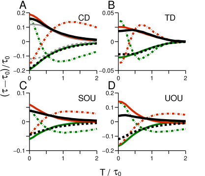
Figure 5: Changes in mean decision times for linear models with lower signal-to-noise ratios. Perturbation protocol is as in Fig. 2. Green (red) curves: perturbation $p$ in the same (opposite) direction as drift rate $b_{0}$; solid: correct choices; dash-dotted: error choices. Solid (dashed) black curves are averages of correct and error choices with perturbation in the same (opposite) direction as drift rate. Grey (black) curves in panel A are for error rate of $0.02\%$ ($5\%$).

Increasing the noise level to $\sigma=7.071$ with thresholds $\zeta=\pm 20$ produces an error rate of $10\%$ in the TD model and changes in mean RTs for correct and error choices similar to those of CD. However, averaged over correct and error choices, overall changes in mean RT exhibit a pattern similar to that of Fig. 2B (see black curves in Fig. 5B). In this respect TD maintains its signature more robustly with increasing error rate than CD, although the effects are progressively masked.

For the SOU model, we increase $\sigma$ to $6.325$, yielding an error rate of $17\%$. The optimal perturbation onset time for changes in mean RT averaged over correct and error trials is masked (compare Fig. 2C with black curves in Fig. 5C). This error rate is relatively high, but we have checked that for error rates as small as $3\%$ SOU model features can also be masked, indicating that, like the CD model, SOU is sensitive to noise.

For the UOU model, more parameters must be adjusted to obtain reasonable RT changes. Here we set $\sigma=2$, $\zeta=\pm 10$, $k=0.02$ and $b_{0}=0.5$, yielding a high error rate of $23.5\%$, but similar trends occur for error rates from $0.1\%$ to $35\%$. Fig. 5D shows that these are comparable to the previous UOU results with high signal-to-noise ratio. Overall, we are unable to distinguish between noise-masking effects and intrinsic features of the UOU integrator.

Using the same parameters, we find that changes in standard deviations for all the linear models show optimal perturbation onset times (Fig. 6). The CD, SOU and UOU models are mutually indistinguishable (cf. Figs. 6A, C and D), but TD exhibits a crossing effect (Fig. 6B) similar to Fig. 3B.

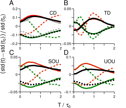
Figure 6: Changes in standard deviations of decision times for the linear models with lower signal-to-noise ratios. Format is as in Figs. 3 and 5.

3.4 Perturbations of the nonlinear model

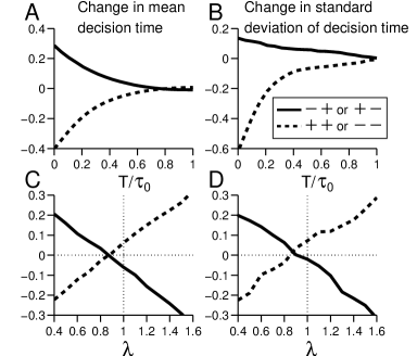
Figure 7: Perturbations of means (left column) and standard deviations (right column) of first passage times for the SPB model. Panels A, B: effects of single pulse perturbations with varying onset times; vertical axes as in Figs. 2 and 3. $-+$ denotes effect of negative pulse at positive threshold, $+-$ denotes effect of positive pulse at negative threshold, etc. Due to symmetry, $-+$ and $+-$ have same effect (solid curves) as do $++$ and $--$ (dashed curves). Panels C, D: responses to zero-effect perturbations; vertical axis in C as in Fig. 4; vertical axis in D shows normalized change in standard deviation as in Fig. 3.

We next apply both perturbation protocols to the nonlinear SPB model. The mean and standard deviation of decision times for the unperturbed system are $80$ and $22$ time units, respectively. The parameters used for the first protocol are given in Table 1, while for the ZEP we set $p=0.005$, $T=30$ and $\Delta T=5$, consistent with application early in the accumulation process. Figs. 7A and B show that the means and standard deviations of decision times behave like those for UOU (cf. panels D of Figs. 2 and 3), decreasing monotonically and approaching zero as onset times increase. ZEPs occur in the pulse ratio range $0.8<\lambda^{*}<1$ for both mean and standard deviation (Figs. 7C and D). Assuming a linear change in mean in Fig. 7C, we find that $\lambda^{*}\approx 0.87$.

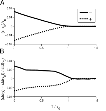
Figure 8: Changes in mean (A) and standard deviation (B) of decision times of the SPB model with high signal-to-noise ratio. All choices are correct. Perturbation protocols and plot formats are as in Figs. 7A and B.

To compare with the behavior of the linear systems in the single threshold case, we now modify the SPB model so that it makes as few errors as they do. This is done by changing $b_{0}$ from $0$ to $0.004$, which breaks the symmetry of the subcritical pitchfork bifurcation (Fig. 1B) so that decisions favor one choice, representing easy tasks (cf. Roxin and Ledberg, (2008)); all other parameters remain the same. Fig. 8 shows that the basic behavior of Figs. 7C and D is preserved: effects on both mean and standard deviation of RTs decrease monotonically as perturbation onset time increases. While the effects on mean passage times of SPB are much like those for UOU, the fact that standard deviations of all four linear models exhibit maxima (Fig. 3) potentially allows us to distinguish SPB from them. The effects of ZEPs in this biased regime is similar to that shown in Figs. 7C and D (data not shown).

4 Discussion

In this work, we have investigated how several simple stochastic integrate-to-threshold decision-making models respond to short perturbations. We focus on two-alternative forced-choice reaction time tasks for which general firing rate models with three coupled neural populations can be reduced to one-dimensional integrate-to-threshold systems. These reduced systems, which may be pure drift-diffusion or Ornstein-Uhlenbeck processes, can be compared analytically and in simulations that require few parameters.

We examined two perturbation protocols, the first being a brief pulse with variable onset time, and the second a pulse-antipulse pair whose amplitude ratio can be adjusted to produce minimal effects (the zero-effect perturbation, ZEP). The simulations of §3 (Figs. 2 and 3) show that the changes in means and standard deviations of decision times allow both perturbation protocols to distinguish between drift-diffusion models and stable and unstable Ornstein-Uhlenbeck processes, provided that perturbations are delivered sufficiently early in the integration process and the signal-to-noise ratio is not too small. Changes in standard deviations can also assist in distinguishing drift-diffusion models with constant drift from those with time-dependent drift rates (cf. Figs. 3A and B), although differences are small and may not be detectable experimentally. (As Ditterich, 2006a notes, entire reaction time distributions can further assist in this.) For early perturbations the ZEP conditions can be approximated analytically, making predictions that are confirmed by computer simulations (Fig. 4). While general analytical expressions for systems with finite noise appear elusive, in Appendix A we prove inequalities for more general nonlinear systems that partially explain our simulation results.

Although we focus on linear models, our methods extend to other systems, and we include results for a nonlinear model that capture the dynamics near a subcritical pitchfork bifurcation which is typical of reduced population models (Wang,, 2002; Wong and Wang,, 2006; Roxin and Ledberg,, 2008). As the results of Appendix A suggest, it behaves in a manner similar to the unstable OU model under both perturbation protocols, although perturbative effects on standard deviations may allow distinctions to be made (Figs. 7-8). We have also confirmed that the TD model’s behavior remains similar with other increasing drift rates (e.g. $b(t)\sim b_{0}t^{2}$; simulation results not shown).

These results reinforce the simulations and claims in Wong et al., (2007) that time-varying perturbations can in principle reveal integration mechanisms. However, some parameter ranges frustrate clear-cut comparisons among models. The first occurs for low signal-to-noise ratios and high error rates (cf. Figs 5-6), and so can be mitigated by using perturbations with more easily discriminated stimuli. Secondly, if there is a ‘dead time’ between stimulus onset and the start of evidence integration, the CD and TD models can display similar signatures to the SOU model, even with high signal-to-noise ratios.

Since perturbations can be delivered through the senses as well as by direct electrical stimulation, the method can be noninvasive and is therefore appropriate for human subjects. Furthermore, unlike fitting neuronal firing rates, both perturbation protocols can distinguish linear and nonlinear UOU-type models (Wang,, 2002; Wong and Wang,, 2006; Roxin and Ledberg,, 2008; Wong and Huk,, 2008) from drift-diffusion models with an ‘urgent’ time-dependent increase in drift rate (Smith et al.,, 2004; Ditterich, 2006a, ; Churchland et al.,, 2008). However, care is required in designing such experiments. Although a high signal-to-noise ratio can in principle help identify integrators, the reaction times can become too short, masking the signature behaviors of the integrators with the ‘thresholding effect’. A possible solution could be to prolong the response deadline in relatively simple reaction time tasks and analyze only data from long RT trials.

Perturbation inputs to decision-making circuits may originate in a single sensory pathway or in other brain areas, as in multisensory and ‘top-down’ inputs (e.g. due to attention (Smith et al.,, 2004; Liu et al.,, 2008)) which could modulate a decision throughout a sensorimotor pathway. The general notion of perturbation developed in the reduced model context extends to such modulatory inputs. The methods may also generalize to other tasks that recruit neural integrators (Goldman et al.,, 2008), such as interval timing (Shea-Brown et al.,, 2006).

Appendix A: Rigorous estimates on first passage times

In this appendix we analyze short single pulse perturbations, First in the noiseless limit, and then with additive noise. The inequalities proved here suggest explanations for the monotonicity of mean first passage times of SOU and UOU processes with respect to early onset times (cf. Figs. 2C and D); moreover, they apply to more general, nonlinear one-dimensional systems such as SPB with thresholds $|\zeta|$ sufficiently close to $X_{t}=0$.

The noiseless limit

As noise amplitude tends to zero, the SDE Eq. 5 becomes an ordinary differential equation (ODE):

$$\frac{dX}{dt}:=\dot{X}=f(X).$$ (17)

Consider two compact perturbations $p$ and $\tilde{p}$ with the same amplitude profile $g(t)$ and duration $\Delta T$, applied at different onset times $T_{1}$ and $\tilde{T}_{1}$:

$$p(t)=1_{[T_{1},T_{2}]}(t)g(t-{T}_{1}),\quad\tilde{p}(t)=1_{[\tilde{T}_{1},\tilde{T}_{2}]}(t)g(t-\tilde{T}_{1})$$ (18)

(here $1_{[T_{1},T_{2}]}$ denotes the indicator function that takes the value 1 for $T_{1}<t<T_{2}$ and zero otherwise). We choose $0<T_{1}<T_{2}<\tilde{T}_{1}<\tilde{T}_{2}$ and $T_{2}-T_{1}=\tilde{T}_{2}-\tilde{T}_{1}=\Delta T$ such that $p$ and $\tilde{p}$ do not overlap and that neither perturbed solution reaches the threshold $X=\zeta$ before $t=\tilde{T}_{2}$. We shall compare solutions $Y_{t}$ and $\tilde{Y}_{t}$ of the corresponding perturbed ODEs,

$$\dot{Y}=f(Y)+p(t)\quad\mbox{and}\quad\dot{\tilde{Y}}=f(\tilde{Y})+\tilde{p}(t),$$ (19)

started at the same initial condition $Y_{0}=\tilde{Y}_{0}=0$, to show how the signs of $f^{\prime}$ and $g$ determine their threshold passage times $\tau$ and $\tilde{\tau}$. We allow smooth nonlinear functions $f$, but assume that $f(X)>0$ for all $0\leq X<\zeta$ and that $g$ does not change sign. The fact that solutions of scalar ODEs cannot cross each other is a key tool.

Lemma 1: Let $X_{t}(x)$ denote the solution of Eq. 17 with initial value $x$. Then $X_{t}(x_{1})<X_{t}(x_{2})$ for any $t>0$ if and only if $x_{1}<x_{2}$.

Proof: This follows from the uniqueness of solutions of ODEs and the ordering of points in a one-dimensional phase space. $\Box$

Since neither perturbation acts after $t=\tilde{T}_{2}$, and neither solution has reached threshold at $\tilde{T}_{2}$, Lemma 1 implies that $\tau<\tilde{\tau}$ if and only if $Y(\tilde{T}_{2})>\tilde{Y}(\tilde{T}_{2})$. We now prove the main result summarized in Table 3, which is a corollary of Proposition 2.

	$f^{\prime}\geq L>0$	$f^{\prime}\leq-L<0$
$g>0$	$\tau<\tilde{\tau}$	$\tau>\tilde{\tau}$
$g<0$	$\tau>\tilde{\tau}$	$\tau<\tilde{\tau}$

Table 3: Monotonicity of first passage dependence on onset time for four sign combinations of $f^{\prime}$ and $g$, in the noise-free limit. $L$ is some constant.

Proposition 2: Assume that the function $g(t)$ in Eqs. 18 is strictly positive for $t\in(0,\Delta T)$. Then for some constant $L$ (a) If $f^{\prime}\geq L>0$, then $Y(t)>\tilde{Y}(t)$ for all $t\geq\tilde{T}_{2}$; (b) If $f^{\prime}\leq-L<0$, then $Y(t)<\tilde{Y}(t)$ for all $t\geq\tilde{T}_{2}$.

Proof of part (a): We need only establish the inequalities at $t=\tilde{T}_{2}$, since no perturbations occur after this time. We compare solutions of Eqs. 19 using the fact that $f(X)>0$ and $f^{\prime}(X)\geq L>0$ for $X\geq 0$ implies that $f(Y)-f(\tilde{Y})\geq L(Y-\tilde{Y})$. Letting $u(t)=Y(t)-\tilde{Y}(t)$ we have

$$\dot{u}=f(Y)-f(\tilde{Y})+p(t)-\tilde{p}(t)\geq Lu+p(t)-\tilde{p}(t).$$ (20)

Since the solutions coincide until the first perturbation occurs at $t=T_{1}$, $u(T_{1})=0$, and integrating inequality 20 over the interval $[T_{1},T_{2}]$, on which $p(t)=g(t-T_{1})$ and $\tilde{p}(t)\equiv 0$, yields:

$$u(T_{2})\geq\int_{T_{1}}^{T_{2}}e^{L(T_{2}-t)}g(t-T_{1})dt>0.$$ (21)

Both $p(t)$ and $\tilde{p}(t)\equiv 0$ on $[T_{2},\tilde{T}_{1}]$, and integration of 20 and use of 21 gives

$$u(\tilde{T}_{1})\geq u(T_{2})e^{L(\tilde{T}_{1}-T_{2})}\geq e^{L(\tilde{T}_{1}-T_{2})}\int_{T_{1}}^{T_{2}}e^{L(T_{2}-t)}g(t-T_{1})dt>0.$$ (22)

Finally, using the fact that $p(t)\equiv 0$ on $[\tilde{T}_{1},\tilde{T}_{2}]$, we integrate 20 again to obtain

$$u(\tilde{T}_{2}) \geq u(\tilde{T}_{1})e^{L(\tilde{T}_{2}-\tilde{T}_{1})}-\int_{\tilde{T}_{1}}^{\tilde{T}_{2}}e^{L(\tilde{T}_{2}-t)}g(t-\tilde{T}_{1})dt$$ (23)

$$\geq \left[e^{L(\tilde{T}_{2}-T_{2})}-1\right]\int_{0}^{\Delta T}e^{L(\Delta T-t)}g(t)dt>0,$$

where we also use inequality 22 and the fact that the additive perturbations of Eq. 18 are identical over the time intervals $[T_{1},T_{2}]$ and $[\tilde{T}_{1},\tilde{T}_{2}]$ to rewrite the integral term. Hence $Y(\tilde{T}_{2})>\tilde{Y}(\tilde{T}_{2})$ and $\tau<\tilde{\tau}$.

Proof of part (b): We again compare solutions of Eqs. 19 but the direction of the inequalities is now reversed, so that we are in essence using Gronwall’s inequality (Guckenheimer and Holmes,, 1983). In this case Eq. 20 becomes

$$\dot{u}\leq-Lu+p(t)-\tilde{p}(t),$$ (24)

inequality 22 becomes

$$u(\tilde{T}_{1})\leq u(T_{2})e^{-L(\tilde{T}_{1}-T_{2})}\leq e^{-L(\tilde{T}_{1}-T_{2})}\int_{T_{1}}^{T_{2}}e^{-L(T_{2}-t)}g(t-T_{1})dt<0,$$ (25)

and the final inequality reads

$$u(\tilde{T}_{2})=Y(\tilde{T}_{2})-\tilde{Y}(\tilde{T}_{2})\leq-\left[1-e^{-L(\tilde{T}_{2}-T_{2})}\right]\int_{0}^{\Delta T}e^{-L(\Delta T-t)}g(t)dt<0.$$ (26)

This implies that $\tau>\tilde{\tau}$, as claimed. Proofs are similar for $g<0$. $\Box$

Extension to noisy systems

The conclusions of Proposition 2 and Table 3 may be extended to apply to expected passage times for SDEs with additive noise. Specifically, replacing Eqns. 19 by

$$dY_{t}=[f(Y_{t})+p(t)]dt+\sigma dW_{t},$$ (27a)

$$d\tilde{Y}_{t}=[f(\tilde{Y}_{t})+\tilde{p}(t)]dt+\sigma d\tilde{W}_{t},$$ (27b)

we have the following result:

Proposition 3: Assume that the function $g(t)$ in Eqs. 18 is strictly positive for $t\in(0,\Delta T)$. Then for some constant $L$ (a) If $f^{\prime}\geq L>0$, then $\mathbb{E}[\tau]<\mathbb{E}[\tilde{\tau}]$; (b) If $f^{\prime}\leq-L<0$, then $\mathbb{E}[\tau]>\mathbb{E}[\tilde{\tau}]$, where $\tau$ and $\tilde{\tau}$ denote the first passage times for Eqns. 27a and 27b respectively.

Proof: We first compare solutions $Y_{t}$ and $\tilde{Y}_{t}$ obtained from Eqns. 27a and 27b under the same sample noise path with increments $d\tilde{W}_{t}\equiv dW_{t}$. Since the stochastic integral $\int_{0}^{t}dW_{t}$ is almost surely continuous (Feller,, 1957), and the integrated noise terms cancel, the comparison of solutions using $u(t)=Y_{t}-\tilde{Y}_{t}$ proceeds as in the deterministic case above, and we conclude that $\tau<\tilde{\tau}$ for $g>0$ and $f^{\prime}\geq L>0$, and $\tau>\tilde{\tau}$ for $g>0$ and $f^{\prime}\leq-L<0$. Finally, averaging each process over an ensemble of sample paths, we may conclude that the mean first passage times of the two processes satisfy similar inequalities to those in the top row of Table 3: $\mathbb{E}[\tau]<\mathbb{E}[\tilde{\tau}]$ and $\mathbb{E}[\tau]>\mathbb{E}[\tilde{\tau}]$ respectively. A similar argument applies to the case $g<0$. $\Box$

Appendix B: A TD model with time-varying perturbation amplitude

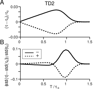
Figure 9: Normalized changes in mean (A) and standard deviation (B) of first passage times for single pulse perturbations with varying onset times applied to a variant of the TD model. Vertical axes and curve conventions are as in Figs. 2 and 3.

In the body of the paper, perturbations of the TD model were assumed unaffected by the time-dependent gain. Here we extend the simulations to a simple case in which perturbation and stimulus (drift) share the same overall linear increase in amplitude. Specifically, we assume the dynamics to be governed by

$$dX_{t}=(b_{0}+p(t))tdt+\sigma dW_{t}.$$ (28)

Otherwise, we change only the perturbation amplitude, taking $p=\pm 2$ instead of $4$. Fig. 9A shows that the changes in mean and standard deviations of exit time for this model remain similar to the previous TD model, but with smaller perturbative effects near the beginning of the trial (quite similar to a SOU model) due to the monotonic time-dependence of perturbation amplitude. However, although the previous pattern of mean exit times no longer applies, the behavior remains qualitatively dissimilar to the CD, UOU and SPB models.

Acknowledgments  We thank C. D. Brody for suggesting a variant of the TD model, M.  Usher and an anonymous reviewer for helpful suggestions that improved the paper, and Nengli Lim for pointing out the extension to noisy systems in Proposition $3$ of Appendix A. XZ was supported in part by ONR grant N00014-01-1-0674, and KFWL and PH by PHS grants MH58480 and MH62196 and AFOSR grant FA9550-07-1-0537. The U.S. Government is authorized to reproduce and distribute reprints for Governmental purposes notwithstanding any copyright notation thereon. The views and conclusions contained herein are those of the authors and should not be interpreted as necessarily representing the official policies or endorsements, either expressed or implied, of the Air Force Research Laboratory or the U.S. Government.

References

- Bogacz et al., (2006) Bogacz, R., Brown, E., Moehlis, J., Holmes, P., and Cohen, J. D. (2006). The physics of optimal decision making: a formal analysis of models of performance in two-alternative forced-choice tasks. Psychol. Rev., 113:700–765.
- Brown et al., (2005) Brown, E., Gao, J., Holmes, P., R. Bogacz, M. G., and Cohen, J. D. (2005). Simple neural networks that optimize decisions. Int. J. Bifurcation and Chaos, 15:803–826.
- Brown and Holmes, (2001) Brown, E. and Holmes, P. (2001). Modeling a simple choice task: stochastic dynamics of mutually inhibitory neural groups. Stochastics and Dynamics, 1:159–191.
- Churchland et al., (2008) Churchland, A. K., Kiani, R., and Shadlen, M. N. (2008). Decision-making with multiple alternatives. Nat. Neurosci., 11:693–702.
- Cohen and Newsome, (2004) Cohen, M. R. and Newsome, W. T. (2004). What electrical microstimulation has revealed about the neural basis of cognition. Curr. Opin. Neurobiol., 14:169–177.
- Ditterch et al., (2003) Ditterch, J., Mazurek, M. E., and Shadlen, M. N. (2003). Microstimulation of visual cortex affects the speed of perceptual decisions. Nat. Neurosci., 6:891–898.
- (7) Ditterich, J. (2006a). Evidence for time-variant decision making. Eur. J. Neurosci., 24:3628–3641.
- (8) Ditterich, J. (2006b). Stochastic models of decisions about motion direction: behavior and physiology. Neural Netw., 19:981–1012.
- Feller, (1957) Feller, W. (1957). An Introduction to Probability Theory and its Applications. Wiley, New York. 2 volumes. Second Edition.
- Gold and Shadlen, (2007) Gold, J. I. and Shadlen, M. N. (2007). The neural basis of decision making. Annu. Rev. Neurosci., 30:535–574.
- Goldman et al., (2008) Goldman, M., Compte, A., and Wang, X.-J. (2008). Theoretical and computational neuroscience: Neural integrators: recurrent mechanisms and models. In Squire, L., Albright, T., Bloom, F., Gage, F., and Spitzer, N., editors, New Encyclopedia of Neuroscience. MacMillan Reference Ltd. In press.
- Guckenheimer and Holmes, (1983) Guckenheimer, J. and Holmes, P. (1983). Nonlinear Oscillations, Dynamical Systems and Bifurcations of Vector Fields. Springer-Verlag, New York.
- Hanes and Schall, (1996) Hanes, D. P. and Schall, J. D. (1996). Neural control of voluntary movement initiation. Science, 274:427–430.
- Hanks et al., (2006) Hanks, T. D., Ditterich, J., and Shadlen, M. N. (2006). Microstimulation of macaque area LIP affects decision-making in a motion discrimination task. Nat. Neurosci., 9:682–689.
- Higham, (2001) Higham, D. J. (2001). An algorithmic introduction to numerical simulation of stochastic differential equations. SIAM Rev., 43:525–546.
- Huk and Shadlen, (2005) Huk, A. C. and Shadlen, M. N. (2005). A neural integrator underlying perceptual decision-making in macaque parietal cortex. J. Neurosci., 25:10420–10436.
- Lindner, (2004) Lindner, B. (2004). Moments of the first passage time under external driving. J. Stat. Phys., 117:703–737.
- Liu et al., (2008) Liu, Y. S., Holmes, P., and Cohen, J. D. (2008). A neural network model of the eriksen task: Reduction, analysis, and data fitting. Neural Comput., 20:345–373.
- Lo and Wang, (2006) Lo, C.-C. and Wang, X.-J. (2006). Cortico-basal ganglia circuit mechanism for a decision threshold in reaction time tasks. Nat. Neurosci., 9:956–963.
- Luce, (1986) Luce, R. D. (1986). Response times: Their Role in Inferring Elementary Mental Organization. Oxford Univ. Press, New York. Oxford Psychology Series, 8.
- Mazurek et al., (2003) Mazurek, M. E., Roitman, J. D., Ditterich, J., and Shadlen, M. N. (2003). A role for neural integrators in perceptual decision making. Cereb Cortex., 13:1257–1269.
- Posner, (1978) Posner, M. I. (1978). Chronometric Explorations of Mind. Erlbaum, Hillsdale, N.J.
- Ratcliff, (1978) Ratcliff, R. (1978). A theory of memory retrieval. Psychol. Rev., 85:59–108.
- Ratcliff, (2006) Ratcliff, R. (2006). Modeling response signal and response time data. Cognit. Psychol., 53:195–237.
- Ratcliff and McKoon, (2008) Ratcliff, R. and McKoon, G. (2008). The diffusion decision model: Theory and data for two-choice decision tasks. Neural Comput., 20:873–922.
- Ratcliff et al., (1999) Ratcliff, R., Zandt, T. V., and McKoon, G. (1999). Connectionist and diffusion models of reaction time. Psychol. Rev., 106:261–300.
- Roitman and Shadlen, (2002) Roitman, J. D. and Shadlen, M. N. (2002). Response of neurons in the lateral intraparietal area during a combined visual discrimination reaction time task. J. Neurosci., 22:9475–9489.
- Roxin and Ledberg, (2008) Roxin, A. and Ledberg, A. (2008). Neurobiological models of two-choice decision making can be reduced to a one-dimensional nonlinear diffusion equation. PLoS Comput. Biol., 4:e1000046.
- Schall, (2003) Schall, J. D. (2003). Neural correlates of decision processes: neural and mental chronometry. Curr. Opin. Neurobiol., 13:182–186.
- Shea-Brown et al., (2006) Shea-Brown, E., Rinzel, J., Rakitin, B. C., and Malapani, C. (2006). A firing rate model of parkinsonian deficits in interval timing. Brain Res., 1070:189–201.
- Simen et al., (2006) Simen, P., Cohen, J. D., and Holmes, P. (2006). Rapid decision threshold modulation by reward rate in a neural network. Neural Netw., 19:1013–1026.
- Smith and Ratcliff, (2004) Smith, P. L. and Ratcliff, R. (2004). Psychology and neurobiology of simple decisions. Trends in Neurosci., 27:161–168.
- Smith et al., (2004) Smith, P. L., Ratcliff, R., and Wolfgang, B. J. (2004). Attention orienting and the time course of perceptual decisions: response time distributions with masked and unmasked displays. Vision Res., 44:1297–1320.
- Strogatz, (2001) Strogatz, S. H. (2001). Nonlinear dynamics and chaos: with applications to physics, biology, chemistry and engineering. Perseus Books Group, Cambridge MA.
- Uhlenbeck and Ornstein, (1930) Uhlenbeck, G. E. and Ornstein, L. S. (1930). On the theory of Brownian motion. Phys. Rev., 36:823–841.
- Usher and McClelland, (2001) Usher, M. and McClelland, J. L. (2001). On the time course of perceptual choice: The leaky competing accumulator model. Psychol Rev., 108:550–592.
- Wang and Uhlenbeck, (1945) Wang, M. C. and Uhlenbeck, G. E. (1945). On the theory of Brownian motion II. Rev. Mod. Phys., 17:323–342.
- Wang, (2002) Wang, X.-J. (2002). Probabilitic decision making by slow reverberation in cortical circuits. Neuron, 36:955–968.
- Wilson and Cowan, (1972) Wilson, H. and Cowan, J. (1972). Excitatory and inhibitory interactions in localized populations of model neurons. Biophys. J, 12:1–24.
- Wilson and Cowan, (1973) Wilson, H. and Cowan, J. (1973). A mathematical theory of the functional dynamics of cortical and thalamic nervous tissue. Kybernetik, 13:55–80.
- Wong and Huk, (2008) Wong, K.-F. and Huk, A. C. (2008). Temporal dynamics underlying perceptual decision making: Insights from the interplay between an attractor model and parietal neurophysiology. Front. Neurosci., 2:245–254.
- Wong et al., (2007) Wong, K.-F., Huk, A. C., Shadlen, M. N., and Wang, X.-J. (2007). Neural circuit dynamics underlying accumulation of time-varying evidence during perceptual decision-making. Front. Comput. Neurosci., 1:6:doi: 10.3389/neuro.10/006.2007.
- Wong and Wang, (2006) Wong, K.-F. and Wang, X.-J. (2006). A recurrent network mechanism of time integration in perceptual decisions. J. Neurosci., 26:1314–1328.