Frequency responses of streamwise-constant
perturbations in channel flows of Oldroyd-B
fluids

Abstract

Non-modal amplification of disturbances in streamwise-constant channel flows of Oldroyd-B fluids is studied from an input-output point of view by analyzing the responses of the velocity components to spatio-temporal body forces. These inputs into the governing equations are assumed to be harmonic in the spanwise direction and stochastic in the wall-normal direction and in time. An explicit Reynolds number scaling of frequency responses from different forcing to different velocity components is developed, showing the same $Re$-dependence as in Newtonian fluids. It is found that some of the frequency response components peak at non-zero temporal frequencies. This is in contrast to Newtonian fluids, where peaks are always observed at zero frequency, suggesting that viscoelastic effects introduce additional timescales and promote development of flow patterns with smaller time constants than in Newtonian fluids. The temporal frequencies, corresponding to the peaks in the components of frequency response, decrease with an increase in viscosity ratio (ratio of solvent viscosity to total viscosity) and show maxima for non-zero elasticity number. Our analysis of the Reynolds-Orr equation demonstrates that the energy-exchange term involving the streamwise/wall-normal polymer stress component $\tau_{xy}$ and the wall-normal gradient of the streamwise velocity $\partial_{y}u$ becomes increasingly important relative to the Reynolds stress term as the elasticity number increases, and is thus the main driving force for amplification in flows with strong viscoelastic effects.

1 Introduction

Complex dynamical responses arise in numerous viscoelastic fluid flows Larson (1992); Shaqfeh (1996) and their study is important from both fundamental and technological standpoints. From the former standpoint, the inception and evolution of amplification of disturbances in various flows involving viscoelastic fluids is not well understood. Viscoelastic effects not only modify features already present in Newtonian fluids, but also give rise to completely new behavioral patterns Larson (2000); Groisman & Steinberg (2000); Bertola et al. (2003). From the latter standpoint, the study of dynamics in flows involving polymeric fluids is of immense importance for polymer processing and rheometry Bird et al. (1987); Larson (1999). Classical linear hydrodynamic stability analysis is found to give misleading results even for simple Couette and Poiseuille flows of Newtonian fluids Schmid (2007). This failure of the classical stability analysis is attributed to the non-normal nature of the generators in the linearized governing equations Trefethen et al. (1993); Grossmann (2000); Schmid & Henningson (2001). Linear dynamical systems with non-normal generators can have solutions that grow substantially at short times, even though they decay at long times Gustavsson (1991); Butler & Farrell (1992); Reddy & Henningson (1993). Furthermore, the non-normal nature of the underlying equations can lead to significant amplification of ambient disturbances Farrell & Ioannou (1993); Bamieh & Dahleh (2001); Jovanović & Bamieh (2005) and substantial decrease of stability margins Trefethen et al. (1993); Trefethen & Embree (2005). On some occasions, the transient growth and amplification, which are overlooked in standard linear stability analysis, could put the system in a regime where nonlinear interactions are no longer negligible. These phenomena are also expected to be important in Couette and Poiseuille flows of viscoelastic fluids. In this paper, we investigate amplification of disturbances in channel flows of Oldroyd-B fluids by performing a frequency-response analysis.

Novel ways of describing fluid stability that allow quantitative description of short-time behavior and disturbance amplification, referred to as non-modal stability analysis, have emerged in the last decade Schmid (2007). One approach is to study the responses of the linearized Navier-Stokes equations (LNSE) to external disturbances Farrell & Ioannou (1993); Bamieh & Dahleh (2001). Jovanović & Bamieh (2005) have used this approach to study the effects of external disturbances, in the form of body forces, on channel flows of Newtonian fluids. Explicit Reynolds number dependence of the components of the frequency response was derived. Based on this finding, it was concluded that at higher Reynolds numbers, wall-normal and spanwise disturbances have the strongest influence on the flow field and the impact of these forces is largest on the streamwise velocity. It was also found that the frequency responses peak at different locations in the ($k_{x},k_{z}$)-plane, where $k_{x}$ and $k_{z}$ are the streamwise and spanwise wavenumbers, indicating the possibility of distinct amplification mechanisms. We note that – even in high-Reynolds-number regimes – it is valid to examine the linearized equations to determine the fate of small-amplitude perturbations to the underlying base flow.

Recently, the present authors have extended the work of Jovanović & Bamieh (2005) to viscoelastic fluids Hoda, Jovanović & Kumar (2008). Prior studies on transient growth phenomena in viscoelastic fluids were reviewed there, and hence will not be reviewed here for brevity. The aggregate effect of stochastic disturbances in all the three spatial directions to all the three velocity components, referred to as the ensemble-average energy density, was investigated. It was found that the energy density increases with an increase in elasticity number and a decrease in viscosity ratio (ratio of solvent viscosity to total viscosity). In most of the cases, streamwise-constant or nearly streamwise-constant perturbations are most amplified and the location of maximum energy density shifts to higher spanwise wavenumbers with an increase in elasticity number and a decrease in viscosity ratio. However, prior work on Newtonian fluids by Jovanović & Bamieh (2005) suggests that a plethora of additional insight can be uncovered by analyzing the componentwise spatio-temporal frequency responses. The componentwise responses give information about the relative importance of the three disturbances on the three velocity components. By analyzing these frequency responses, the disturbance frequency corresponding to maximum amplification can also be obtained.

In this paper, we examine the componentwise frequency responses in streamwise-constant channel flows of Oldroyd-B fluids. This study supplements a previous study by the authors (Hoda et al., 2008), where the aggregate effect of disturbances was examined, and helps in understanding the relative importance of the disturbances on the different velocity components. Because the previous study focused on aggregate effects, as parameterized by the energy density, it leaves open the question of exactly which velocity components are most amplified and which forcing components are responsible for this amplification. Furthermore, since the energy density is a time-integrated quantity, it does not yield information about most amplified temporal frequencies. The present work addresses these issues, provides some explicit scaling relationships, and further investigates physical mechanisms.

Streamwise-constant three-dimensional perturbations are considered in this work as they are most amplified by the linearized dynamics. We derive an explicit Reynolds number scaling for the components of the frequency response. As in Newtonian fluids, at higher Reynolds numbers the forces in the wall-normal and spanwise directions have the strongest influence on the flow field and the impact of these forces is largest on the streamwise velocity. In some of the cases, the frequency response components peak at non-zero temporal frequencies. This is distinct from Newtonian fluids, where peaks are always observed at zero frequency, suggesting that elasticity introduces additional timescales and promotes development of flow patterns with smaller time constants than in Newtonian fluids. We also find that the temporal frequencies, corresponding to the peaks in the components of frequency response, decrease with an increase in viscosity ratio and show maxima with respect to the elasticity number. One of the most important conclusions of this paper is the observation that elasticity can lead to considerable energy amplification even when inertial effects are weak; this energy amplification may then serve as a route through which channel flows of Oldroyd-B fluids transition to turbulence at low Reynolds numbers (Larson, 2000; Groisman & Steinberg, 2000).

Our presentation is organized as follows: in § 2, a model for streamwise-constant channel flows of Oldroyd-B fluids with external forcing is presented. In § 3, a brief summary of the notion of the spatio-temporal frequency response is provided. In § 4, an explicit scaling of the frequency response components with the Reynolds number is given. In § 5 and § 6, the effects of elasticity number and viscosity ratio on power spectral and steady-state energy densities are studied. The important findings are summarized in § 7, and the detailed mathematical derivations are relegated to the Appendix.

2 The cross-sectional 2D/3C model

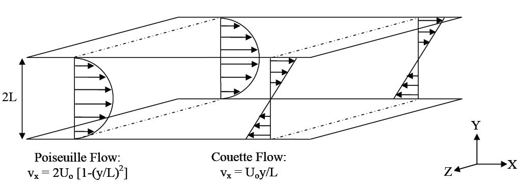
Figure 1: Schematic of the channel-flow geometry.

A schematic of the channel-flow geometry is shown in figure 1. The height of the channel is $2L$ and the channel extends infinitely in the $x$- and $z$- directions. For Couette flow, the top plate moves in the positive $x$-direction and the bottom plate moves in the negative $x$-direction, each with uniform velocity $U_{o}$. For Poiseuille flow, $2U_{o}$ is the centerline velocity. We analyze the dynamical properties of the LNSE for an Oldroyd-B fluid with spatially distributed and temporally varying body-force fields. The parameters characterizing Oldroyd-B fluids are: (a) the viscosity ratio, $\beta=\eta_{s}/(\eta_{s}+\eta_{p})$, where $\eta_{s}$ and $\eta_{p}$ are the solvent and polymer viscosities, respectively; (b) the Reynolds number, $Re=U_{o}L/\nu=\rho U_{o}L/(\eta_{s}+\eta_{p})$, which represents the ratio of inertial to viscous forces, where $\rho$ denotes fluid density; (c) the Weissenberg number, $W\!e=\lambda U_{o}/L$, which characterizes the importance of the fluid relaxation time, $\lambda$, with respect to the characteristic flow time, $L/U_{o}$. Another important parameter is the elasticity number, $\mu=W\!e/Re=\lambda\nu/L^{2}$, which quantifies the ratio between the fluid relaxation time, $\lambda$, and the vorticity diffusion time, $L^{2}/\nu$.

Consider the dimensionless linearized momentum, continuity, and constitutive equations

$$\begin{array}[]{rcl}\partial_{t}\mathbf{v}&\!\!=\!\!&-\;\mathbf{v}\cdot\mbox{\boldmath$\nabla$}\mathbf{\overline{v}}\;-\;\mathbf{\overline{v}}\cdot\mbox{\boldmath$\nabla$}\mathbf{v}\;+\;\dfrac{1}{Re}\Bigl{(}-\mbox{\boldmath$\nabla$}p\;+\;\beta\nabla^{2}\mathbf{v}\;+\;(1-\beta)\mbox{\boldmath$\nabla$}\cdot\mbox{\boldmath${\tau}$}\Bigr{)}\;+\;\mathbf{d},\\[-2.84544pt] 0&\!\!=\!\!&\mbox{\boldmath$\nabla$}\cdot\mathbf{v},\\[0.0pt] \partial_{t}\mbox{\boldmath${\tau}$}&\!\!=\!\!&\dfrac{1}{W\!e}\bigl{(}\mbox{\boldmath$\nabla$}\mathbf{v}\;+\;\left(\mbox{\boldmath$\nabla$}\mathbf{v}\right)^{T}\bigr{)}\;-\;\mathbf{v}\cdot\mbox{\boldmath$\nabla$}\mbox{\boldmath${\overline{\tau}}$}\;-\;\mathbf{\overline{v}}\cdot\mbox{\boldmath$\nabla$}\mbox{\boldmath$\tau$}\;+\;\mbox{\boldmath${\tau}$}\cdot\mbox{\boldmath$\nabla$}\mathbf{\overline{v}}\;+\;\mbox{\boldmath${\overline{\tau}}$}\cdot\mbox{\boldmath$\nabla$}\mathbf{v}\\ &\!\!+\!\!&(\mbox{\boldmath${\overline{\tau}}$}\cdot\mbox{\boldmath$\nabla$}\mathbf{v})^{T}\;+\;(\mbox{\boldmath${\tau}$}\cdot\mbox{\boldmath$\nabla$}\mathbf{\overline{v}})^{T}\;-\;\dfrac{\mbox{\boldmath${\tau}$}}{W\!e},\end{array}$$ (1)

where $\mathbf{v}=\left[~{}u~{}~{}v~{}~{}w~{}\right]^{T}$ is the velocity fluctuation vector, $p$ is the pressure fluctuation, and ${\tau}$ is the polymer stress fluctuation. The overbar denotes the base flow given by

$$\mathbf{\overline{v}}~{}=~{}\left[~{}U(y)~{}~{}0~{}~{}0~{}\right]^{T},~{}~{}~{}\overline{\mbox{\boldmath{$\tau$}}}~{}=~{}\left[\begin{array}[]{c c c}2W\!e\left(U^{\prime}(y)\right)^{2}&U^{\prime}(y)&0\\[0.0pt] U^{\prime}(y)&0&0\\[0.0pt] 0&0&0\end{array}\right],$$

with $U(y)\,=\,\{y,~{}\mbox{Couette flow};$ $1-y^{2},~{}\mbox{Poiseuille flow}\},$ and $U^{\prime}(y)=\mathrm{d}U(y)/\mathrm{d}y$. A spatio-temporal body force is represented by ${\bf d}=\left[~{}d_{1}~{}~{}d_{2}~{}~{}d_{3}~{}\right]^{T}$, where $d_{1},d_{2}$, and $d_{3}$ are the body force fluctuations in the streamwise ($x$), wall-normal ($y$), and spanwise ($z$) directions, respectively. These body forces can be either deterministic or stochastic, and they serve as inputs into the system of equations that governs evolution of velocity and polymer stress fluctuations Jovanović & Bamieh (2005). Our objective is to investigate their effect on the components of the velocity field ${\bf v}=\left[~{}u~{}~{}v~{}~{}w~{}\right]^{T}$.

In this paper, we confine our analysis to streamwise-constant perturbations. In this special case, the model for flow perturbations is usually referred to as the two-dimensional, three-component (2D/3C) model Reynolds & Kassinos (1995). (2D indicates that the dynamics evolve in the cross-sectional ($y,z$)-plane, and 3C indicates that velocity components in all three spatial directions are considered.) The motivation for a thorough analysis of this particular model is twofold: (a) a recent study by the authors suggests that streamwise-constant (and nearly streamwise-constant) perturbations in channel flows of Oldroyd-B fluids create the largest contribution to the ensemble-average energy density Hoda et al. (2008); and (b) for the 2D/3C model, an explicit $Re$-dependence for the components of the frequency response can be obtained, which clarifies the effectiveness (energy content) of forcing (velocity) components.

The evolution model of the forced linearized system (1) with streamwise-constant perturbations ($k_{x}=0$) is obtained by a standard conversion (Schmid & Henningson, 2001) to the wall-normal velocity/vorticity ($v,\omega_{y}$) formulation:

$$\begin{array}[]{rcl}\partial_{t}\mbox{\boldmath$\psi$}(y,k_{z},t)&\!\!=\!\!&\left[\,\mathbf{A}(k_{z})\mbox{\boldmath$\psi$}(k_{z},t)\,\right](y)\;+\;\left[\,\bar{\mathbf{B}}(k_{z})\mathbf{d}(k_{z},t)\,\right](y),\\[2.84544pt] {\bf v}(y,k_{z},t)&\!\!=\!\!&\left[\,\mathbf{C}(k_{z})\mbox{\boldmath$\psi$}_{1}(k_{z},t)\,\right](y).\end{array}$$ (2)

Here, $k_{z}$ is the spanwise wavenumber, $\mbox{\boldmath$\psi$}=\left[~{}\mbox{\boldmath$\psi$}_{1}^{T}~{}~{}\mbox{\boldmath$\psi$}_{2}^{T}~{}\right]^{T},$ $\mbox{\boldmath$\psi$}_{1}=\left[~{}v~{}~{}\omega_{y}~{}\right]^{T}$, and the components of polymer stress are given by $\mbox{\boldmath$\psi$}_{2}=\left[\,\tau_{xx}~{}\tau_{yy}~{}\tau_{zz}~{}\tau_{xy}~{}\tau_{xz}~{}\tau_{yz}\,\right]^{T}.$ The derivation of the evolution equation for $v$ requires elimination of the pressure from Eqs. (1). This is achieved by applying the divergence operator to the momentum equation and by combining the resulting equation with continuity. On the other hand, the equation for $\omega_{y}$ is derived by applying the curl operator to the momentum equation.

The operator $\mathbf{A}$ in Eq. (2) is referred to as the dynamical generator of the linearized dynamics and it characterizes internal properties of the LNSE (e.g., modal stability). The definition of this operator for full three-dimensional fluctuations is provided in Hoda et al. (2008); the definition of components of this operator suitable for frequency response analysis of the 2D/3C model is given in Eqs. (3) and (4) below. We also note that operator $\bar{\mathbf{B}}$ can be partitioned as $\bar{\mathbf{B}}=\left[~{}\mathbf{B}^{T}~{}~{}\mathbf{O}^{T}~{}\right]^{T},$ where $\mathbf{B}$ describes how forcing enters into the Orr-Sommerfeld and Squire equations of viscoelastic channel flows, and $\mathbf{O}$ is a $6\times 3$ matrix of null operators. On the other hand, operator $\mathbf{C}$ in Eq. (2) contains information about a kinematic relationship between $\mbox{\boldmath$\psi$}_{1}$ and ${\bf v}$. These two operators are given by:

$$\mathbf{B}~{}=~{}\left[\begin{array}[]{ccc}0&\mathbf{B}_{2}&\mathbf{B}_{3}\\[0.0pt] \mathbf{B}_{1}&0&0\end{array}\right],~{}~{}~{}\mathbf{C}~{}=~{}\left[\begin{array}[]{cc}0&\mathbf{C}_{u}\\[0.0pt] \mathbf{C}_{v}&0\\[0.0pt] \mathbf{C}_{w}&0\end{array}\right],$$

$$\{\mathbf{B}_{1}=\mathrm{i}k_{z},\,\mathbf{B}_{2}=-k^{2}_{z}{\mbox{\boldmath$\Delta$}}^{-1},\,\mathbf{B}_{3}=-\mathrm{i}k_{z}{\mbox{\boldmath$\Delta$}}^{-1}\partial_{y}\},~{}\{\mathbf{C}_{u}=-(\mathrm{i}/k_{z}),\,\mathbf{C}_{v}=\mathbf{I},\,\mathbf{C}_{w}=(\mathrm{i}/k_{z})\partial_{y}\},$$

where $\mathrm{i}=\sqrt{-1}$, $\mathbf{I}$ is the identity operator, $\mbox{\boldmath$\Delta$}=\partial_{yy}-k_{z}^{2}$ is a Laplacian with Dirichlet boundary conditions, and $\mbox{\boldmath$\Delta$}^{-1}$ denotes the inverse of the Laplacian. System (2) is subject to the following boundary conditions $\{v(\pm 1,k_{z},t)=\partial_{y}v(\pm 1,k_{z},t)=\omega_{y}(\pm 1,k_{z},t)=0\},$ which come from the no-slip and no-penetration requirements. We note that no boundary conditions on the polymer stresses are needed Hoda et al. (2008).

A coordinate transformation $\mbox{\boldmath$\phi$}=\mathbf{T}\mbox{\boldmath$\psi$}$ with $\{\phi_{1}=v,$ $\mbox{\boldmath$\phi$}_{2}=\left[\,\tau_{yy}~{}\tau_{yz}~{}\tau_{zz}\,\right]^{T},$ $\phi_{3}=\omega_{y},$ $\mbox{\boldmath$\phi$}_{4}=\left[\,\tau_{xy}~{}\tau_{xz}\,\right]^{T},$ $\phi_{5}=\tau_{xx}\}$ can be used to bring system (2) into the following form:

$$\partial_{t}\,\phi_{1} ~{}=~{}\dfrac{\beta}{Re}\,\mathbf{F}_{11}\,\phi_{1}~{}+~{}\dfrac{1\,-\,\beta}{Re}\,\mathbf{F}_{12}\,\mbox{\boldmath$\phi$}_{2}~{}+~{}\mathbf{B}_{2}\,d_{2}~{}+~{}\mathbf{B}_{3}\,d_{3},$$ (3a)

$$\partial_{t}\,\mbox{\boldmath$\phi$}_{2} ~{}=~{}-\dfrac{1}{\mu Re}\,\mbox{\boldmath$\phi$}_{2}~{}+~{}\dfrac{1}{\mu Re}\,\mathbf{F}_{21}\,\phi_{1},$$ (3b)

$$\partial_{t}\,\phi_{3} ~{}=~{}\dfrac{\beta}{Re}\,\mathbf{F}_{33}\,\phi_{3}~{}+~{}\mathbf{F}_{31}\,\phi_{1}~{}+~{}\dfrac{1\,-\,\beta}{Re}\,\mathbf{F}_{34}\,\mbox{\boldmath$\phi$}_{4}~{}+~{}\mathbf{B}_{1}\,d_{1},$$ (3c)

$$\partial_{t}\,\mbox{\boldmath$\phi$}_{4} ~{}=~{}-\dfrac{1}{\mu Re}\,\mbox{\boldmath$\phi$}_{4}~{}+~{}\mathbf{F}_{41}\,\phi_{1}~{}+~{}\mathbf{F}_{42}\,\mbox{\boldmath$\phi$}_{2}~{}+~{}\dfrac{1}{\mu Re}\,\mathbf{F}_{43}\,\phi_{3},$$ (3d)

$$\partial_{t}\,\phi_{5} ~{}=~{}-\dfrac{1}{\mu Re}\,\phi_{5}~{}-~{}{\mu Re}\,\mathbf{F}_{51}\,\phi_{1}~{}+~{}\mathbf{F}_{53}\,\phi_{3}~{}+~{}\mathbf{F}_{54}\,\mbox{\boldmath$\phi$}_{4},$$ (3e)

$$\left[\begin{array}[]{c}{u}\\[0.0pt] {v}\\[0.0pt] {w}\end{array}\right] ~{}=~{}\left[\begin{array}[]{cc}0&\mathbf{C}_{u}\\[0.0pt] \mathbf{C}_{v}&0\\[0.0pt] \mathbf{C}_{w}&0\end{array}\right]\left[\begin{array}[]{c}{\phi_{1}}\\[0.0pt] {\phi_{3}}\end{array}\right],$$ (3n)

where the $\mathbf{F}$-operators are given by:

$$\begin{array}[]{c}\mathbf{F}_{11}\;=\;\mbox{\boldmath$\Delta$}^{-1}\mbox{\boldmath$\Delta$}^{2},~{}~{}\mathbf{F}_{33}\;=\;\mbox{\boldmath$\Delta$},~{}~{}\mathbf{F}_{31}\;=\;-\,\mathrm{i}k_{z}U^{\prime}(y),\\[4.26773pt] \mathbf{F}_{12}\;=\;\mbox{\boldmath$\Delta$}^{-1}\left[\begin{array}[]{ccc}-k_{z}^{2}\partial_{y}&-\mathrm{i}k_{z}\left(\partial_{yy}\,+\,k_{z}^{2}\right)&k_{z}^{2}\partial_{y}\end{array}\right],~{}~{}\mathbf{F}_{34}\;=\;\left[\begin{array}[]{cc}\mathrm{i}k_{z}\partial_{y}&-k_{z}^{2}\end{array}\right],\\[4.26773pt] \mathbf{F}_{21}\;=\;\left[\begin{array}[]{ccc}2\partial_{y}&(\mathrm{i}/k_{z})\left(\partial_{yy}\,+\,k_{z}^{2}\right)&-2\partial_{y}\end{array}\right]^{T},~{}~{}\mathbf{F}_{43}\;=\;-\,(1/k_{z}^{2})\mathbf{F}_{34}^{T},\\[4.26773pt] \mathbf{F}_{41}\;=\;\left[\begin{array}[]{c}U^{\prime}(y)\partial_{y}-U^{\prime\prime}(y)\\[0.0pt] (\mathrm{i}/k_{z})U^{\prime}(y)\partial_{yy}\end{array}\right],~{}~{}\mathbf{F}_{42}\;=\;\left[\begin{array}[]{ccc}U^{\prime}(y)&0&0\\[0.0pt] 0&U^{\prime}(y)&0\end{array}\right],\\[7.11317pt] \mathbf{F}_{51}\;=\;4U^{\prime}(y)U^{\prime\prime}(y),~{}~{}\mathbf{F}_{53}\;=\;-\,(2\mathrm{i}/k_{z})U^{\prime}(y)\partial_{y},~{}~{}\mathbf{F}_{54}\;=\;\left[\begin{array}[]{cc}2U^{\prime}(y)&0\end{array}\right].\end{array}$$ (4)

Here, $\mbox{\boldmath$\Delta$}^{2}=\partial_{yyyy}-2k_{z}^{2}\partial_{yy}+k_{z}^{4}$ with both Dirichlet and Neumann boundary conditions.

The system of equations (3) is in a form suitable for the analysis performed in § 4 where an explicit characterization of the Reynolds-number dependence for the components of the frequency response of system (2) is provided. It is noteworthy that for the 2D/3C model there is no coupling from $\phi_{5}\,=\,\tau_{xx}$ to the equations for the other flow-field components in (3); in particular, this demonstrates that evolution of $\tau_{xx}$ at $k_{x}=0$ does not influence evolution of $u$, $v$, and $w$. We also note a one-way coupling from Eqs. (3a) and (3b) to Eqs. (3c) and (3d); this indicates that the dynamical properties of $\phi_{3}=\omega_{y}$ and $\mbox{\boldmath$\phi$}_{4}=\left[\,\tau_{xy}~{}\tau_{xz}\,\right]^{T}$ are influenced by $\phi_{1}=v$ and $\mbox{\boldmath$\phi$}_{2}=\left[\,\tau_{yy}~{}\tau_{yz}~{}\tau_{zz}\,\right]^{T}$ but not vice-versa.

3 Frequency responses for streamwise-constant perturbations

Frequency response represents a cornerstone of input-output analysis of linear dynamical systems Zhou et al. (1996). The utility of input-output analysis in understanding early stages of transition in wall-bounded shear flows of Newtonian fluids is by now well documented; we refer the reader to a recent review article by Schmid (2007) for more information. It turns out that the input-output approach also reveals important facets of transitional dynamics in channel flows of Oldroyd-B fluids Hoda et al. (2008).

To provide a self-contained treatment, we next present a brief summary of the notion of the spatio-temporal frequency response of the streamwise-constant LNSE with forcing; we invite the reader to see Jovanović & Bamieh (2005) for additional details. The spatio-temporal frequency response of system (2) is given by

$$\mathbf{H}(k_{z},\omega)~{}=~{}\mathbf{C}(k_{z})(\mathrm{i}\omega\mathbf{I}-\mathbf{A}(k_{z}))^{-1}\bar{\mathbf{B}}(k_{z}),$$

where $\omega$ denotes the temporal frequency. The frequency response is obtained directly from the Fourier symbols of the operators in Eq. (2), and for any pair ($k_{z},\omega$) it represents an operator (in $y$) that maps the forcing field into the velocity field.

The frequency response of a system with a stable generator $\mathbf{A}$ describes the steady-state response to harmonic input signals across temporal and spatial frequencies. Since $\mathbf{H}$ is an operator valued function of two independent variables $k_{z}$ and $\omega$, there are a variety of ways to visualize its properties. In this paper, we study the Hilbert–Schmidt norm of $\mathbf{H}$

$$\Pi(k_{z},\omega)\;=\;\mathrm{trace}\left(\mathbf{H}(k_{z},\omega)\mathbf{H}^{*}(k_{z},\omega)\right),$$ (5)

where $\mathbf{H}^{*}$ represents the adjoint of operator $\mathbf{H}$. For any pair $(k_{z},\omega)$, the Hilbert–Schmidt norm quantifies the power spectral density of the velocity field in the LNSE subject to harmonic (in $z$) white, unit variance, temporally stationary, stochastic (in $y$ and $t$) body forcing. Furthermore, the temporal-average of the power spectral density of $\mathbf{H}$ yields the so-called $H_{2}$ norm of system (2) (Zhou et al., 1996)

$$E(k_{z})\;=\;\dfrac{1}{2\pi}\int_{-\infty}^{\infty}\Pi(k_{z},\omega)\,\mathrm{d}\omega.$$

The frequency responses of viscoelastic channel flows (as a function of $k_{x}$ and $k_{z}$) are quantified in Hoda et al. (2008) in terms of the $H_{2}$ norm. We note that at any $k_{z}$, the $H_{2}$ norm determines the energy (variance) amplification of harmonic (in $z$) stochastic (in $y$ and $t$) disturbances Farrell & Ioannou (1993); Bamieh & Dahleh (2001); Jovanović & Bamieh (2005). This quantity is also known as the ensemble-average energy density of the statistical steady-state Farrell & Ioannou (1993), and it is hereafter referred to as the (steady-state) energy density (or energy amplification).

We finally note that the frequency response of system (2), ${\bf v}=\mathbf{H}{\bf d}$, has the following $3\times 3$ block-decomposition:

$$\left[\begin{array}[]{c}u\\[0.0pt] v\\[0.0pt] w\end{array}\right]=\left[\begin{array}[]{ccc}\mathbf{H}_{u1}(k_{z},\omega;Re,\beta,\mu)&\mathbf{H}_{u2}(k_{z},\omega;Re,\beta,\mu)&\mathbf{H}_{u3}(k_{z},\omega;Re,\beta,\mu)\\[0.0pt] \mathbf{H}_{v1}(k_{z},\omega;Re,\beta,\mu)&\mathbf{H}_{v2}(k_{z},\omega;Re,\beta,\mu)&\mathbf{H}_{v3}(k_{z},\omega;Re,\beta,\mu)\\[0.0pt] \mathbf{H}_{w1}(k_{z},\omega;Re,\beta,\mu)&\mathbf{H}_{w2}(k_{z},\omega;Re,\beta,\mu)&\mathbf{H}_{w3}(k_{z},\omega;Re,\beta,\mu)\end{array}\right]\left[\begin{array}[]{c}d_{1}\\[0.0pt] d_{2}\\[0.0pt] d_{3}\end{array}\right],$$ (6)

which is suitable for uncovering the effectiveness (energy content) of forcing (velocity) components. In this representation, $\mathbf{H}_{rj}$ denotes the frequency response operator from $d_{j}$ to $r$, with $\{j=1,2,3;$ $r=u,v,w\}$. Our notation suggests that $\!-\!$ in addition to the spanwise wavenumber $k_{z}$ and the temporal frequency $\omega$ $\!-\!$ each component of $\mathbf{H}$ also depends on the Reynolds number $Re$, the viscosity ratio $\beta$, and the elasticity number $\mu$.

4 Dependence of frequency responses on the Reynolds number

In this section, we study how the power spectral densities and the steady-state energy densities scale with $Re$ for each of the components of the frequency response (6). Furthermore, the square-additive property of these two quantities is used to determine the aggregate effect of forces in all three spatial directions ${\bf d}=\left[~{}d_{1}~{}~{}d_{2}~{}~{}d_{3}~{}\right]^{T}$ on all three velocity components ${\bf v}=\left[~{}u~{}~{}v~{}~{}w~{}\right]^{T}$. We analytically establish that the frequency responses from both wall-normal and spanwise forces to streamwise velocity scale as $Re^{2}$, while the frequency responses of all other components in Eq. (6) scale at most as $Re$. This extends the Newtonian-fluid results (Jovanović, 2004; Jovanović & Bamieh, 2005) to channel flows of Oldroyd-B fluids.

Application of the temporal Fourier transform to Eq. (3) facilitates elimination of polymer stresses from the 2D/3C model (see Appendix A for details). This leads to an equivalent representation of system (3) in terms of its block diagram, which is shown in figure 2 with $\Omega=\omega Re$. From this block diagram, it follows that operator $\mathbf{H}(k_{z},\omega;Re,\beta,\mu)$ in Eq. (6) can be expressed as

$$\left[\begin{array}[]{c}u\\[0.0pt] v\\[0.0pt] w\end{array}\right]=\left[\begin{array}[]{cll}Re\,\bar{\mathbf{H}}_{u1}(k_{z},\Omega;\beta,\mu)&Re^{2}\,\bar{\mathbf{H}}_{u2}(k_{z},\Omega;\beta,\mu)&Re^{2}\,\bar{\mathbf{H}}_{u3}(k_{z},\Omega;\beta,\mu)\\[0.0pt] 0&Re\,\bar{\mathbf{H}}_{v2}(k_{z},\Omega;\beta,\mu)&Re\,\bar{\mathbf{H}}_{v3}(k_{z},\Omega;\beta,\mu)\\[0.0pt] 0&Re\,\bar{\mathbf{H}}_{w2}(k_{z},\Omega;\beta,\mu)&Re\,\bar{\mathbf{H}}_{w3}(k_{z},\Omega;\beta,\mu)\end{array}\right]\left[\begin{array}[]{c}d_{1}\\[0.0pt] d_{2}\\[0.0pt] d_{3}\end{array}\right],$$ (7)

where the Reynolds-number-independent operators $\bar{\mathbf{H}}$ are given by:

$$\begin{array}[]{rcl}\bar{\mathbf{H}}_{u1}(k_{z},\Omega;\beta,\mu)&\!=\!&\mathbf{C}_{u}(\mathrm{i}\Omega\mathbf{I}\,-\,\mathbf{S})^{-1}\mathbf{B}_{1},\\[4.26773pt] \bar{\mathbf{H}}_{uj}(k_{z},\Omega;\beta,\mu)&\!=\!&\mathbf{C}_{u}(\mathrm{i}\Omega\mathbf{I}\,-\,\mathbf{S})^{-1}\mathbf{C}_{p}(\mathrm{i}\Omega\mathbf{I}\,-\,\mathbf{L})^{-1}\mathbf{B}_{j},~{}~{}~{}j=2,3,\\[4.26773pt] \bar{\mathbf{H}}_{rj}(k_{z},\Omega;\beta,\mu)&\!=\!&\mathbf{C}_{r}(\mathrm{i}\Omega\mathbf{I}\,-\,\mathbf{L})^{-1}\mathbf{B}_{j},~{}~{}~{}\{r=v,w;\;j=2,3\}.\end{array}$$

Operators $\mathbf{L}$, $\mathbf{S}$, and $\mathbf{C}_{p}$ are defined by:

$$\begin{array}[]{c}\mathbf{L}\;=\;\dfrac{1\,+\,\mathrm{i}\beta\mu\Omega}{1\,+\,\mathrm{i}\mu\Omega}\mbox{\boldmath$\Delta$}^{-1}\mbox{\boldmath$\Delta$}^{2},~{}~{}~{}\mathbf{S}\;=\;\dfrac{1\,+\,\mathrm{i}\beta\mu\Omega}{1\,+\,\mathrm{i}\mu\Omega}\mbox{\boldmath$\Delta$},~{}~{}~{}\mathbf{C}_{p}\;=\;\mathbf{C}_{p1}\,+\,\dfrac{\mu}{(1\,+\,\mathrm{i}\mu\Omega)^{2}}\mathbf{C}_{p2},\\[7.11317pt] \mathbf{C}_{p1}\;=\;-\mathrm{i}k_{z}U^{\prime}(y),~{}~{}~{}\mathbf{C}_{p2}\;=\;\mathrm{i}k_{z}(1\,-\,\beta)\left(U^{\prime}(y)\mbox{\boldmath$\Delta$}\,+\,2U^{\prime\prime}(y)\partial_{y}\right).\end{array}$$

In the limit $\beta\rightarrow 1$, these operators simplify to the familiar Orr-Sommerfeld ($\mbox{\boldmath$\Delta$}^{-1}\mbox{\boldmath$\Delta$}^{2}$), Squire ($\Delta$), and coupling ($-\mathrm{i}k_{z}U^{\prime}(y)$) operators in the streamwise-constant LNSE of Newtonian fluids with $Re=1$. We note that even though viscoelastic effects modify some of the operators in figure 2, there is a striking similarity between block-diagram representations of the 2D/3C models of non-Newtonian and Newtonian fluids Jovanović & Bamieh (2005). In particular, figure 2 shows that the frequency responses from $d_{2}$ and $d_{3}$ to $u$ scale as $Re^{2}$, whereas the responses from all other forcing components to other velocity components scale linearly with $Re$. It should be noted that the frequency responses of Newtonian fluids at $k_{x}\,=\,0$ show same scaling with $Re$ Jovanović (2004); Jovanović & Bamieh (2005). The coupling operator, $\mathbf{C}_{p}$, is crucial for the $Re^{2}$-scaling. In Newtonian fluids $\mathbf{C}_{p}$ corresponds to the vortex tilting term, $\mathbf{C}_{p1}$; in viscoelastic fluids $\mathbf{C}_{p}$ also contains an additional term, $\mathbf{C}_{p2}$, that captures the coupling from the wall-normal velocity to the wall-normal vorticity due to the work done by the polymer stresses on the flow. In the absence of the coupling operator, all the components of $\mathbf{H}(\omega,k_{z};Re,\beta,\mu)$ scale at most linearly with $Re$. Figure 2 also suggests that for the 2D/3C model, streamwise forcing does not influence the wall-normal and spanwise velocities, which is in agreement with Newtonian-fluid results (Jovanović & Bamieh, 2005). As noted in Appendix A, $\mathbf{C}_{p2}$ has its origin in the term involving polymer stress fluctuations and gradients in the base velocity profile. This would produce polymer stretching, and could be interpreted as giving rise to an effective lift-up mechanism (Landahl, 1975).

Figure 2: Block diagram representation of the streamwise constant LNS system (2).

The $Re$-scaling for the power spectral densities of operators $\mathbf{H}_{rj}(k_{z},\omega;Re,\beta,\mu)$ in streamwise-constant Poiseuille and Couette flows of Oldroyd-B fluids follows directly from Eqs. (5) and (7) and linearity of the trace operator:

$$\left[\begin{array}[]{ccc}\Pi_{u1}(k_{z},\omega;Re,\beta,\mu)&\Pi_{u2}(k_{z},\omega;Re,\beta,\mu)&\Pi_{u3}(k_{z},\omega;Re,\beta,\mu)\\[0.0pt] \Pi_{v1}(k_{z},\omega;Re,\beta,\mu)&\Pi_{v2}(k_{z},\omega;Re,\beta,\mu)&\Pi_{v3}(k_{z},\omega;Re,\beta,\mu)\\[0.0pt] \Pi_{w1}(k_{z},\omega;Re,\beta,\mu)&\Pi_{w2}(k_{z},\omega;Re,\beta,\mu)&\Pi_{w3}(k_{z},\omega;Re,\beta,\mu)\end{array}\right]$$ (8)

$$={} \left[\begin{array}[]{ccc}{\bar{\Pi}_{u1}(k_{z},\Omega;\beta,\mu)Re^{2}}&{\bar{\Pi}_{u2}(k_{z},\Omega;\beta,\mu)Re^{4}}&{\bar{\Pi}_{u3}(k_{z},\Omega;\beta,\mu)Re^{4}}\\[0.0pt] {0}&{\bar{\Pi}_{v2}(k_{z},\Omega;\beta,\mu)Re^{2}}&{\bar{\Pi}_{v3}(k_{z},\Omega;\beta,\mu)Re^{2}}\\[0.0pt] {0}&{\bar{\Pi}_{w2}(k_{z},\Omega;\beta,\mu)Re^{2}}&{\bar{\Pi}_{w3}(k_{z},\Omega;\beta,\mu)Re^{2}}\end{array}\right],$$

where $\bar{\Pi}_{rj}$ are the power spectral densities of the Reynolds-number-independent operators $\bar{\mathbf{H}}_{rj}(k_{z},\Omega;\beta,\mu)$, with $\Omega\,=\,\omega Re$. Furthermore, the power spectral density of operator $\mathbf{H}(k_{z},\omega;Re,\beta,\mu)$, ${\bf v}\,=\,\mathbf{H}{\bf d}$, is given by

$$\Pi(k_{z},\omega;Re,\beta,\mu)\;=\;\bar{\Pi}_{a}(k_{z},\Omega;\beta,\mu)Re^{2}\;+\;\bar{\Pi}_{b}(k_{z},\Omega;\beta,\mu)Re^{4},$$

where $\bar{\Pi}_{a}\,=\,\bar{\Pi}_{u1}\,+\,\bar{\Pi}_{v2}\,+\,\bar{\Pi}_{v3}\,+\,\bar{\Pi}_{w2}\,+\,\bar{\Pi}_{w3}$ and $\bar{\Pi}_{b}\,=\,\bar{\Pi}_{u2}\,+\,\bar{\Pi}_{u3}.$

Several important observations can be made about Eq. (8) without doing any detailed calculations. First, the power spectral densities of operators $\mathbf{H}_{u2}$ and $\mathbf{H}_{u3}$ scale as $Re^{4}$; in all other cases they scale at most as $Re^{2}$. This illustrates the dominance of the streamwise velocity perturbations and the forces in the wall-normal and spanwise directions in high-Reynolds-number channel flows of streamwise constant Oldroyd-B fluids. Second, apart from $\bar{\Pi}_{u2}(k_{z},\Omega;\beta,\mu)$ and $\bar{\Pi}_{u3}(k_{z},\Omega;\beta,\mu)$, the other power spectral densities in Eq. (8) do not depend on the base velocity and stresses. These two power spectral densities depend on the coupling operator, $\mathbf{C}_{p}$, and thus their values differ in Poiseuille and Couette flows. Third, power spectral densities $\bar{\Pi}_{rj}(k_{z},\Omega;\beta,\mu)$ do not depend on the Reynolds number. Thus, $Re$ only affects the magnitudes of $\Pi_{rj}(k_{z},\omega;Re,\beta,\mu)$, and regions of temporal frequencies $\omega$ where these power spectral densities peak. As $Re$ increases, these $\omega$-regions shrink as $1/Re$. Therefore, for high-Reynolds-number channel flows of Oldroyd-B fluids, the influence of small temporal frequencies dominates the evolution of the velocity perturbations, suggesting preeminence of the effects in fluids with relatively large time constants. It is noteworthy that elasticity shifts temporal frequencies where $\bar{\Pi}_{rj}$ peak to higher values, which is discussed in detail in § 5. For additional details concerning these points, we refer the reader to Hoda (2008).

We next exploit the above results to establish the Reynolds-number dependence of steady-state energy densities for different components of frequency response operator (6). For example, $E_{u2}(k_{z};Re,\beta,\mu)$ is determined by

$$\begin{array}[]{rll}E_{u2}(k_{z};Re,\beta,\mu)&\!=\!&\displaystyle{\dfrac{1}{2\pi}\int_{-\infty}^{\infty}}\Pi_{u2}(\omega,k_{z};Re,\beta,\mu)\,\mathrm{d}\omega\\[9.95863pt] &\!=\!&\displaystyle{\dfrac{Re^{4}}{2\pi}\int_{-\infty}^{\infty}}\bar{\Pi}_{u2}(\Omega,k_{z};\beta,\mu)\,\mathrm{d}\omega\\[9.95863pt] &\!=\!&\displaystyle{\dfrac{Re^{3}}{2\pi}\int_{-\infty}^{\infty}}\bar{\Pi}_{u2}(\Omega,k_{z};\beta,\mu)\,\mathrm{d}\Omega\\[9.95863pt] &\!=:\!&Re^{3}g_{u2}(k_{z};\beta,\mu).\end{array}$$

A similar procedure can be used to determine the steady-state energy densities of all other components of operator $\mathbf{H}$ in Eq. (6), which yields:

$$\left[\begin{array}[]{lll}E_{u1}(k_{z};Re,\beta,\mu)&E_{u2}(k_{z};Re,\beta,\mu)&E_{u3}(k_{z};Re,\beta,\mu)\\[0.0pt] E_{v1}(k_{z};Re,\beta,\mu)&E_{v2}(k_{z};Re,\beta,\mu)&E_{v3}(k_{z};Re,\beta,\mu)\\[0.0pt] E_{w1}(k_{z};Re,\beta,\mu)&E_{w2}(k_{z};Re,\beta,\mu)&E_{w3}(k_{z};Re,\beta,\mu)\end{array}\right]$$

$$={} \left[\begin{array}[]{ccc}{f_{u1}(k_{z};\beta,\mu)Re}&{g_{u2}(k_{z};\beta,\mu)Re^{3}}&{g_{u3}(k_{z};\beta,\mu)Re^{3}}\\[0.0pt] {0}&{f_{v2}(k_{z};\beta,\mu)Re}&{f_{v3}(k_{z};\beta,\mu)Re}\\[0.0pt] {0}&{f_{w2}(k_{z};\beta,\mu)Re}&{f_{w3}(k_{z};\beta,\mu)Re}\end{array}\right],$$

where $f_{rj}$ and $g_{rj}$ are functions independent of $Re$. Furthermore, the steady-state energy density of operator $\mathbf{H}(k_{z},\omega;Re,\beta,\mu)$, ${\bf v}\,=\,\mathbf{H}{\bf d}$, is given by

$$E(k_{z};Re,\beta,\mu)\;=\;f(k_{z};\beta,\mu)Re\;+\;g(k_{z};\beta,\mu)Re^{3},$$ (9)

where $f\,=\,f_{u1}\,+\,f_{v2}\,+\,f_{v3}\,+\,f_{w2}\,+\,f_{w3}$ and $g\,=\,g_{u2}\,+\,g_{u3}.$

We conclude that energy amplification from both spanwise and wall-normal forcing to streamwise velocity is $O(Re^{3})$, while energy amplification for all other components is $O(Re)$.

5 Parametric study of power spectral densities

In § 4, we derived an explicit dependence for each component of the frequency response operator (6) on the Reynolds number. Here, we investigate the effect of $\beta$ and $\mu$ on the ($\Omega$, $k_{z}$)-parameterized plots of power spectral densities $\bar{\Pi}_{rj}$, $\{r=u,v,w;$ $j=1,2,3\}$, by setting $Re=1$ in Eq. (8). In all the plots presented in this section, $100\times 90$ logarithmically spaced grid points are used in the $(\Omega,k_{z})$-plane. The temporal frequency and spanwise wavenumber are varied between $0.01$ and $25.11$ ($\Omega$) and $0.1$ and $15.84$ ($k_{z}$), respectively. The Reynolds-number-independent power spectral densities $\bar{\Pi}_{rj}(k_{z},\Omega;\beta,\mu)$ in Eq. (8) can either be numerically determined from a finite-dimensional approximation of the underlying operators or they can be computed using the method developed by Jovanović & Bamieh (2006). For numerical approximation, we use a Chebyshev collocation technique (Weideman & Reddy, 2000); between $30$ and $50$ collocation points were found to be sufficient to obtain accurate results. In Couette flow, the power spectral densities can be computed more efficiently using the method developed by Jovanović & Bamieh (2006). This can be accomplished by expressing each component of the frequency response operator in a different form, known as the two-point boundary value state-space realization (Hoda, 2008). In Couette flow, we used both methods for evaluating $\bar{\Pi}_{rj}$; the results agreed with each other, suggesting accuracy of our computations.

Figures 3 and 4, respectively, show the ($\Omega,k_{z}$)-dependence of the $Re$-independent power spectral densities $\bar{\Pi}_{rj}$ in Eq. (8), for $\beta\,=\,0.1$ and $\mu\,=\,10$. As noted in § 4, only $\bar{\Pi}_{u2}$ and $\bar{\Pi}_{u3}$ depend on the base velocity and polymer stresses. In view of this, the results in figure 4 are computed in both Couette and Poiseuille flows. Since, at $k_{x}=0$, $d_{1}$ does not affect $v$ and $w$, we do not plot $\bar{\Pi}_{v1}$ and $\bar{\Pi}_{w1}$ in figure 3. Also, since $\bar{\Pi}_{w2}\,=\,\bar{\Pi}_{v3}$, we only plot $\bar{\Pi}_{v3}(k_{z},\Omega;\beta,\mu)$. We now discuss some important observations concerning the results presented in these figures.

It is clearly seen that several frequency-response components peak at non-zero $\Omega$ values. This is in contrast to Newtonian fluids, where all power spectral densities attain their respective maxima at $\Omega\,=\,0$ Jovanović & Bamieh (2006). Also, since the peaks for different components of the frequency response are observed at different locations in the $(\Omega,k_{z})$-plane, these plots suggest distinct amplification mechanisms. It is worth mentioning that the locations of the peaks shift depending upon the $\beta$ and $\mu$ values. Our results indicate that viscoelastic effects introduce additional timescales which promote development of spatio-temporal flow patterns with smaller time constants compared to Newtonian fluids.

At low $Re$ values $(\leq 1)$, depending upon $\mu$, either input-output amplification from $d_{1}$ to $u$ attains the largest value or the amplification from ($d_{2},d_{3}$) to $u$ attains the largest value. At small values of $\mu$, $\bar{\Pi}_{u1}$ has the largest magnitude; this suggests that at small Reynolds numbers and small elasticity numbers, the streamwise forcing has the strongest influence (on the velocity) and the most powerful impact of this forcing is on the streamwise velocity component. At higher values of $\mu$, $\bar{\Pi}_{u2}$ and $\bar{\Pi}_{u3}$ achieve the largest magnitudes; this suggests that at higher elasticity numbers, the spanwise and wall-normal forces have the strongest influence (on the velocity) and that the streamwise velocity component is most energetic.

$\bar{\Pi}_{u1}(k_{z},\Omega;\beta,\mu)$	$\bar{\Pi}_{v2}(k_{z},\Omega;\beta,\mu)$
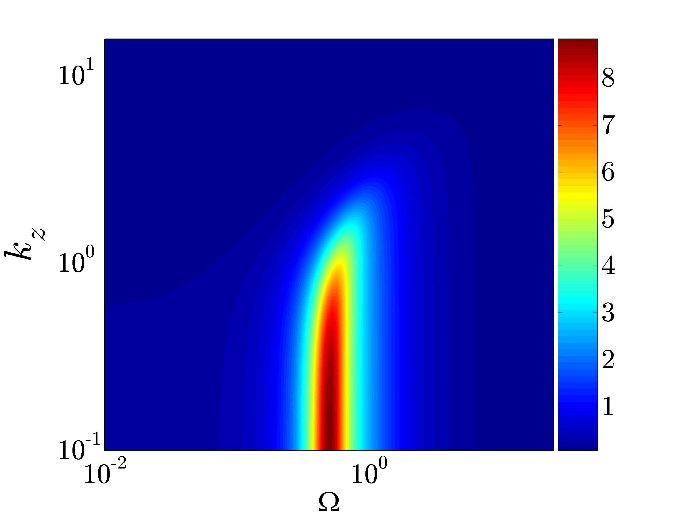
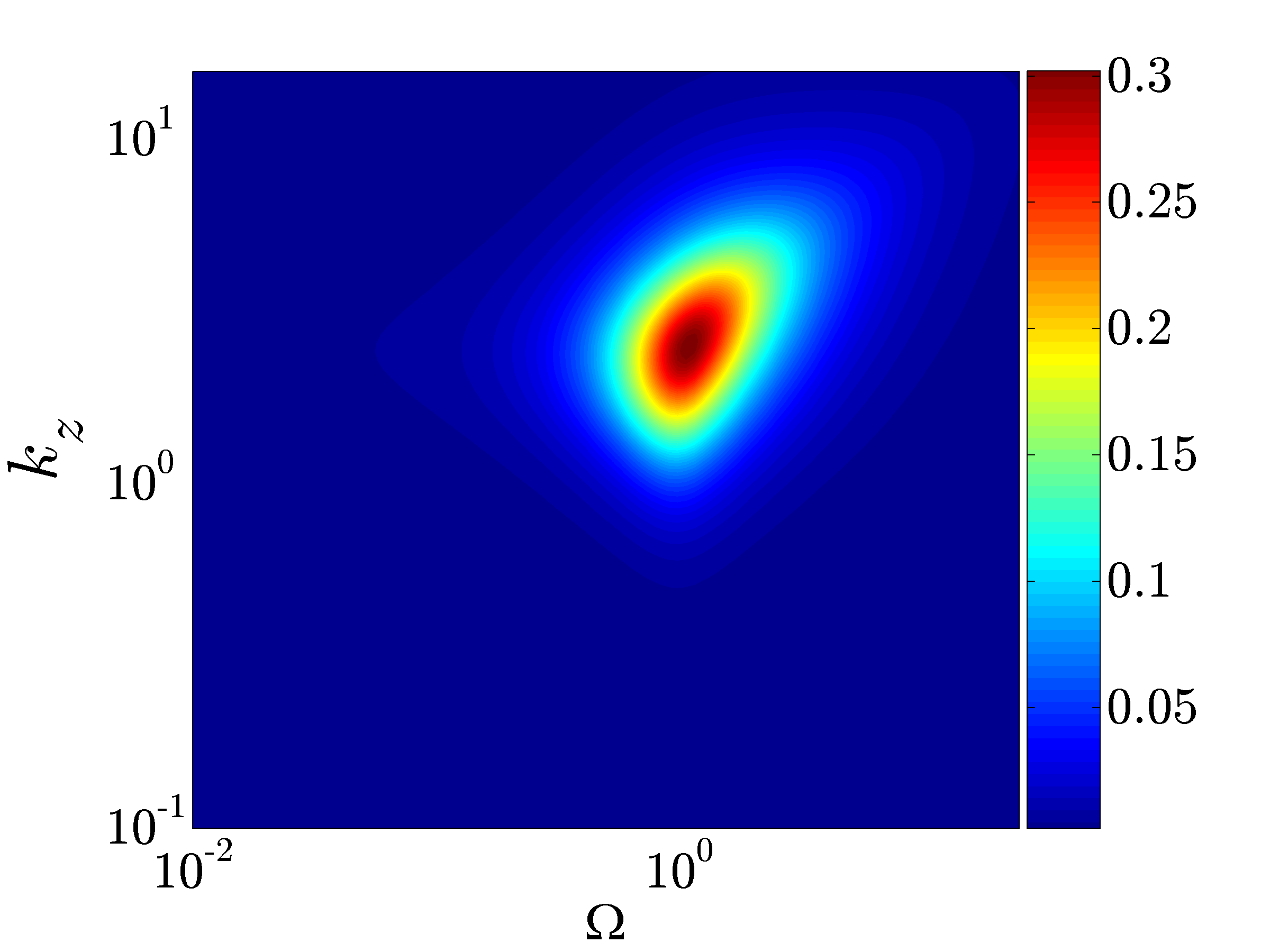
$\bar{\Pi}_{v3}(k_{z},\Omega;\beta,\mu)$	$\bar{\Pi}_{w3}(k_{z},\Omega;\beta,\mu)$

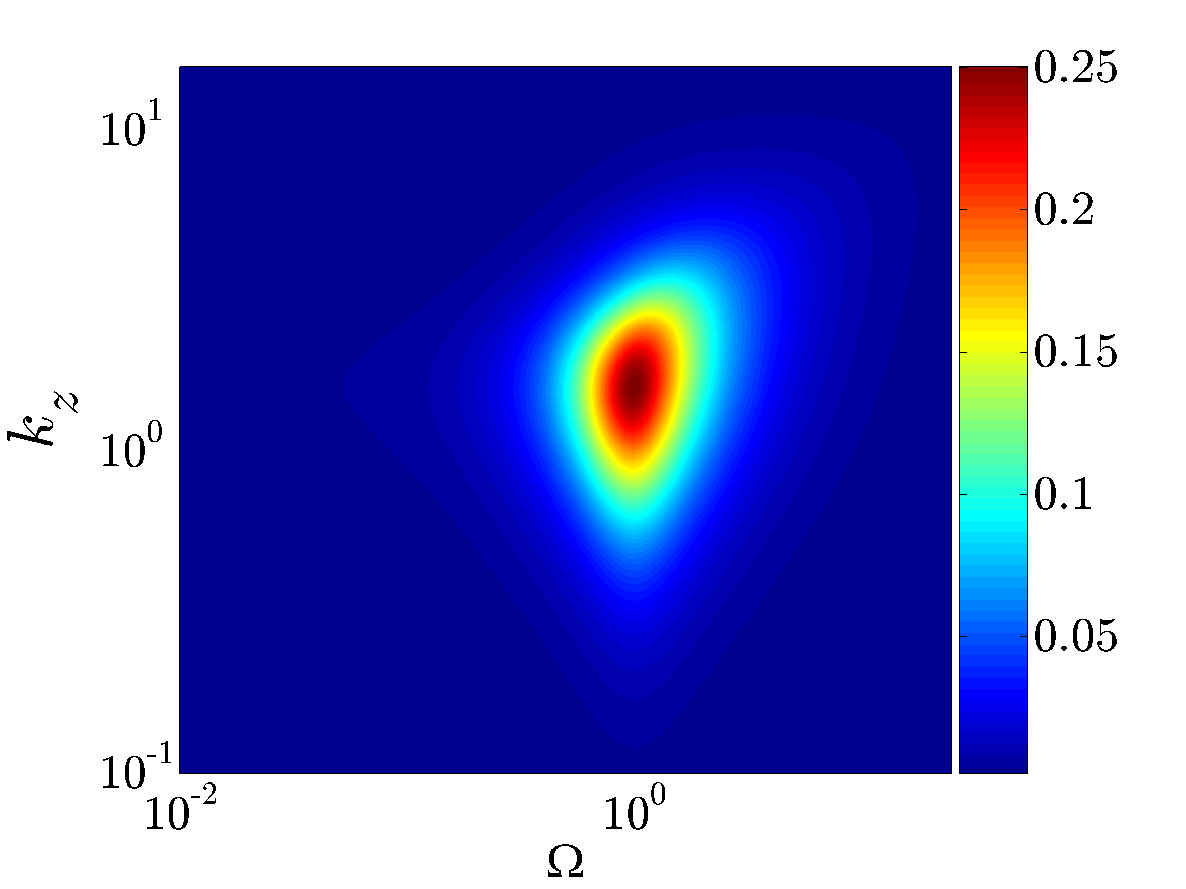
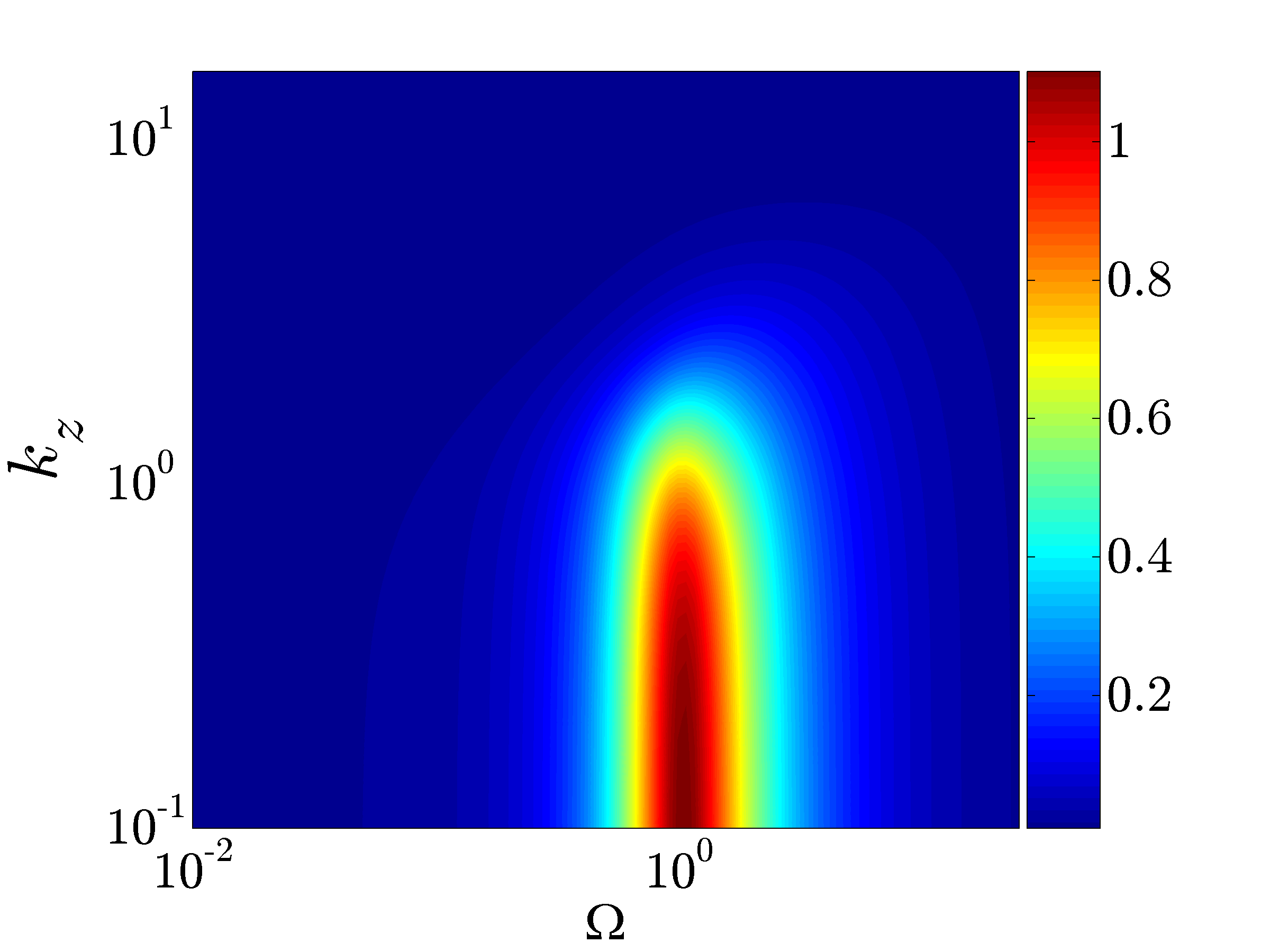
Figure 3: Plots of the base-flow-independent power spectral densities $\bar{\Pi}_{rj}$ in Eq. (8) for $\beta\,=\,0.1$, $\mu\,=\,10$.

$\bar{\Pi}_{u2}(k_{z},\Omega;\beta,\mu)$	$\bar{\Pi}_{u3}(k_{z},\Omega;\beta,\mu)$
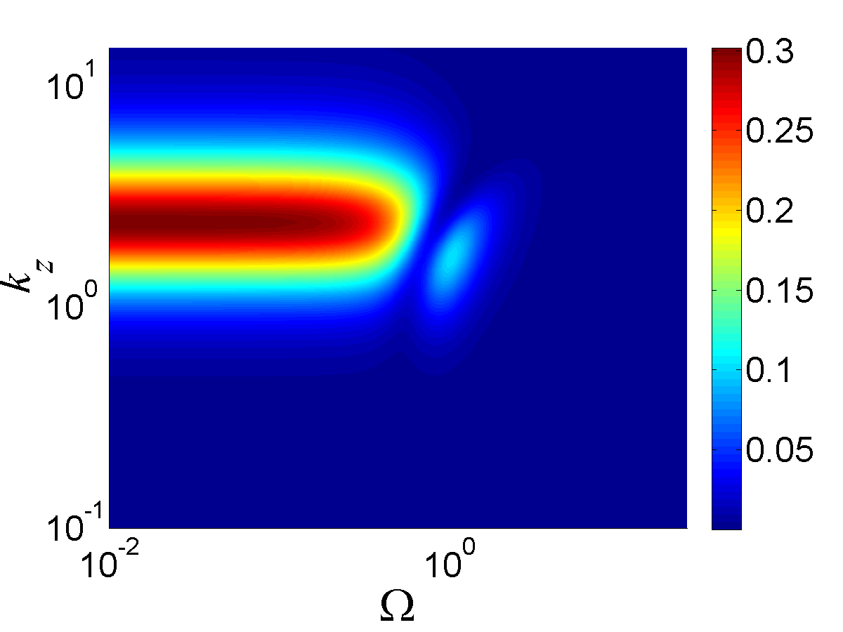
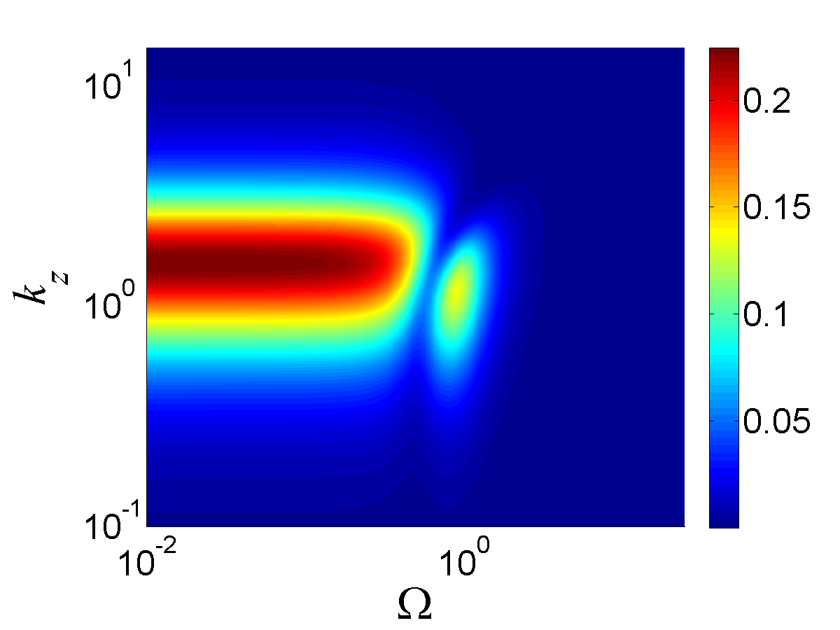
$\bar{\Pi}_{u2}(k_{z},\Omega;\beta,\mu)$	$\bar{\Pi}_{u3}(k_{z},\Omega;\beta,\mu)$

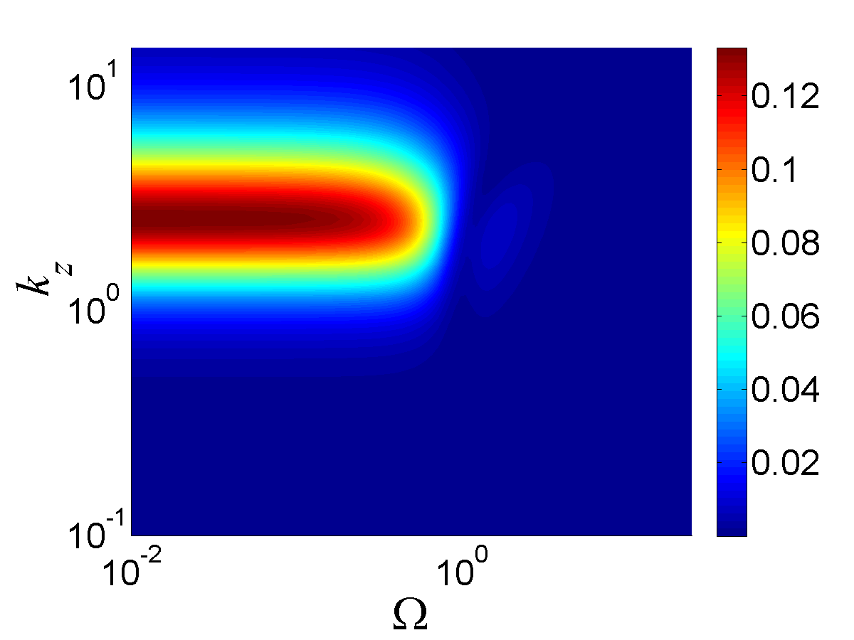
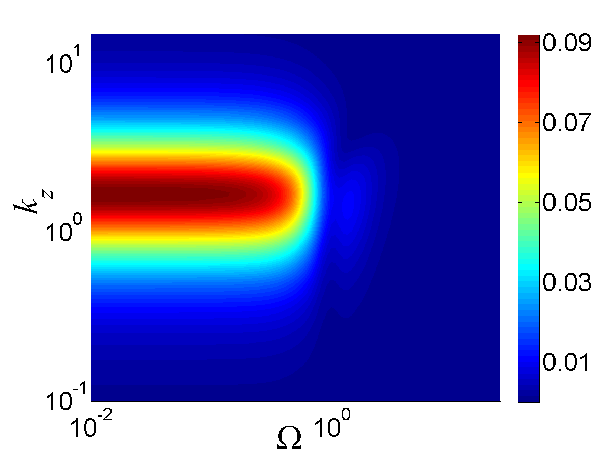
Figure 4: Plots of the base-flow-dependent power spectral densities $\bar{\Pi}_{u2}$ and $\bar{\Pi}_{u3}$ in Eq. (8) for Couette (first row) and Poiseuille (second row) flows with $\beta\,=\,0.1$, $\mu\,=\,10$.

As discussed above, the power spectral density peaks (for different components of the frequency response operator) are observed at different locations in the $(\Omega,k_{z})$-plane. We next analyze the effects of parameters $\mu$ and $\beta$ on the magnitude of these peaks and the locations of the respective maxima. Figures 5 and 6, respectively, illustrate the variation with $\mu$ (for $\beta=\{0,1$, $0.5$, $0.9\}$) in the $\Omega$-value corresponding to the maxima of functions $\bar{\Pi}_{rj}$ in Eq. (8); we denote this value by $\Omega_{\max}$. Below, we discuss the key features of these results.

For $\mu$ greater than a certain threshold value, $\Omega_{\max}$ exhibits a maximum in $\mu$. Also, the value of $\mu$ corresponding to the maximum in $\Omega_{\max}$ decreases with a decrease in $\beta$. The above results suggest that for a particular range of elasticity numbers, viscoelastic effects in Oldroyd-B fluids promote amplification of flow structures with smaller time constants than in Newtonian fluids. For small elasticity numbers, figures 5 and 6 demonstrate that all power spectral densities achieve their peak values at zero temporal frequency. This is consistent with the behavior of Newtonian fluids Jovanović & Bamieh (2006) as an Oldroyd-B fluid is equivalent to a Newtonian fluid in the limit $\mu\,\rightarrow\,0$. The plots in figure 5 also suggest that for large elasticity numbers, $\Omega_{\max}$ monotonically decreases (with a slow rate of decay) as $\mu$ increases.

It is also seen that $\Omega_{\max}$ increases with a decrease in $\beta$, suggesting the importance of effects with shorter time constants in viscoelastic fluids. In the limit $\beta\,\rightarrow\,1$, $\Omega_{\max}\,=\,0$ (results not shown), which is in agreement with the behavior of Newtonian fluids Jovanović & Bamieh (2006); an Oldroyd-B fluid is equivalent to a Newtonian fluid in the limit $\beta\,\rightarrow\,1$.

For the base-flow-independent power spectral densities in Eq. (8), a very good analytical estimate for $\Omega_{\max}$ can be determined by projecting the operators in $\mathbf{H}_{rj}$ on the first eigenfunctions of $\mbox{\boldmath$\Delta$}^{-1}\mbox{\boldmath$\Delta$}^{2}$ (for $\bar{\Pi}_{rj}$, $\{r=v,w;\;j=2,3\}$) and $\Delta$ (for $\bar{\Pi}_{u1}$). (We refer the reader to Appendix B of Jovanović & Bamieh (2005) for spectral analysis of these two operators in the 2D/3C model.) Using this approach, we determine the following expression for $\Omega_{\max}$

$$\Omega_{\max}\;=\;\left\{\begin{array}[]{cl}\dfrac{\sqrt{{\sqrt{\mu|\lambda_{1}(k_{z})|(1-\beta)(\mu|\lambda_{1}(k_{z})|(1+\beta)+2)}}\,-\,1}}{\mu},&\text{$\mu\,>\,\dfrac{\sqrt{\frac{2}{1\,-\,\beta}}\,-\,1}{|\lambda_{1}(k_{z})|(1+\beta)}$},\\[7.11317pt] 0,&\text{otherwise,}\end{array}\right.$$

where $\lambda_{1}(k_{z})$ is the principal eigenvalue of the underlying operator ($\Delta$ for $\bar{\Pi}_{u1}$; $\mbox{\boldmath$\Delta$}^{-1}\mbox{\boldmath$\Delta$}^{2}$ for $\bar{\Pi}_{rj}$, $\{r=v,w;\;j=2,3\}$). From this expression, it follows that $\Omega_{\max}$ increases with a decrease in $\beta$ and that it exhibits a maximum in $\mu$, explaining the trends observed in figure 5. Furthermore, for $\mu\,\gg\,1$, $\Omega_{\max}$ approximately scales as $1/\sqrt{\mu}$, which justifies our earlier claim regarding the slow rate of decay of $\Omega_{\max}$ with $\mu$ for large elasticity numbers.

$\bar{\Pi}_{u1}(k_{z},\Omega;\beta,\mu)$	$\bar{\Pi}_{v2}(k_{z},\Omega;\beta,\mu)$
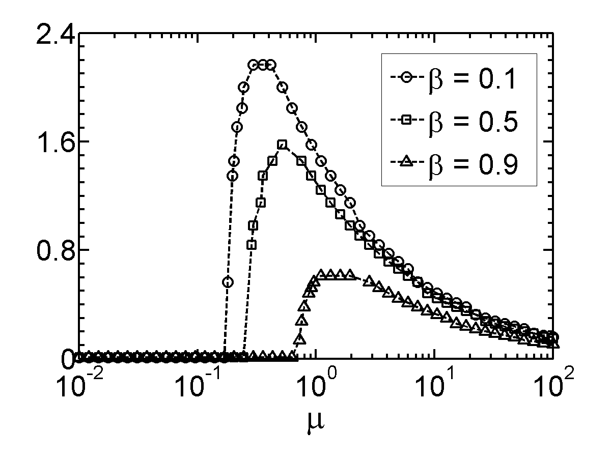
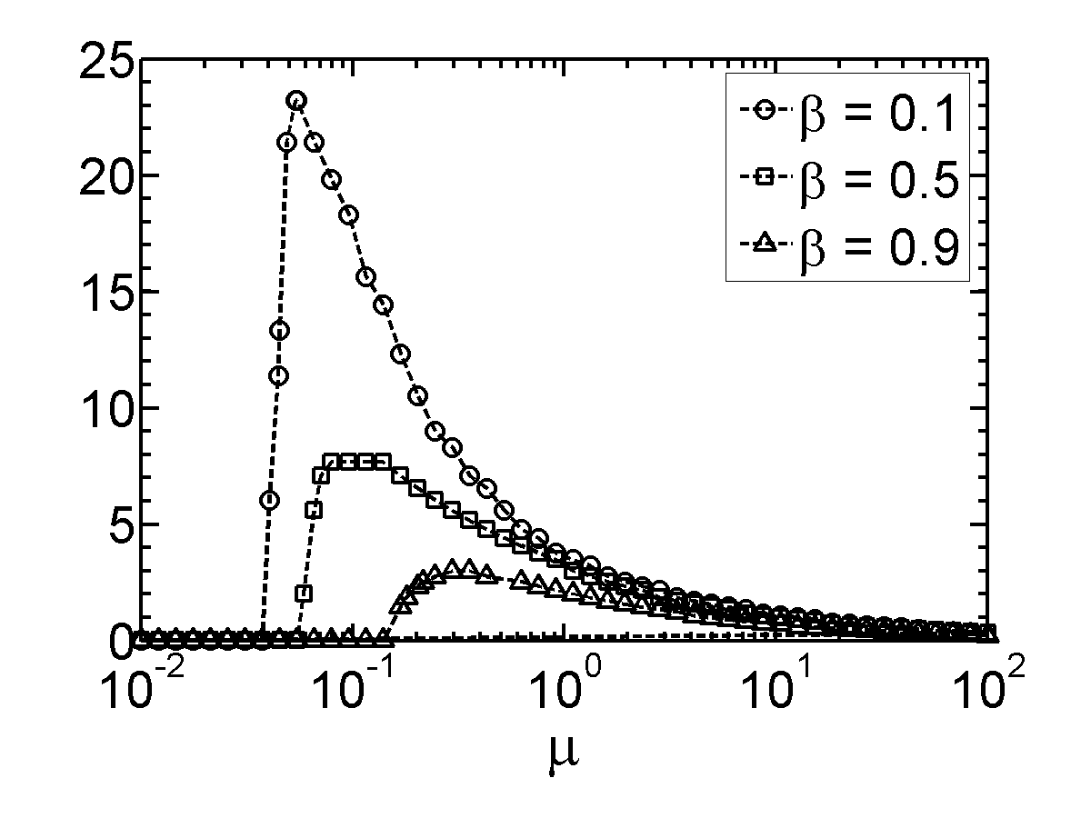
$\bar{\Pi}_{v3}(k_{z},\Omega;\beta,\mu)$	$\bar{\Pi}_{w3}(k_{z},\Omega;\beta,\mu)$

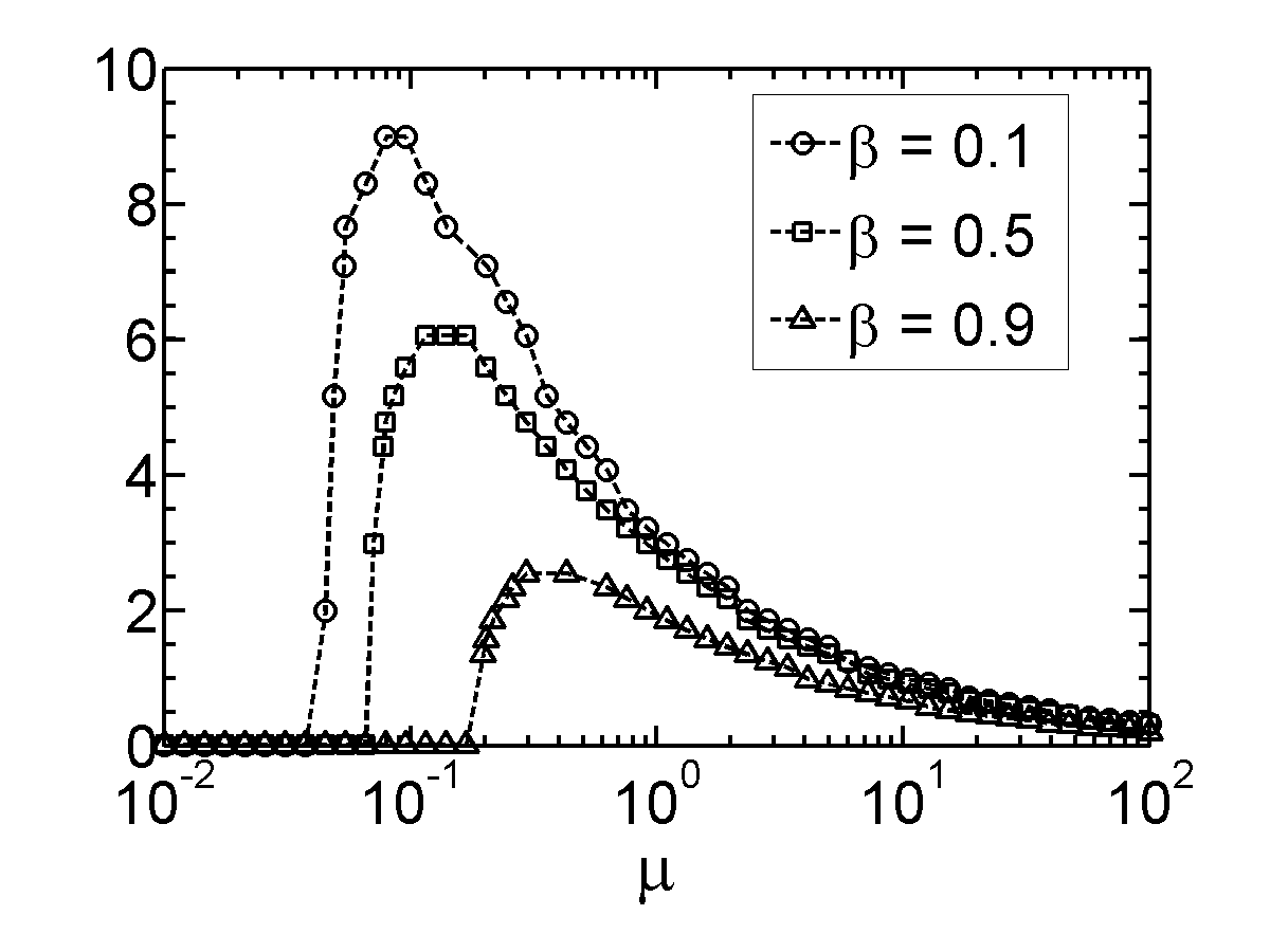
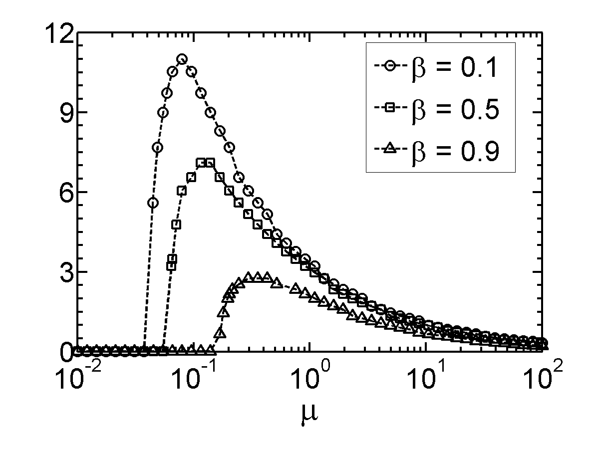
Figure 5: Variation in $\Omega_{\max}$ with $\mu$ for $\beta\,=\,\{0.1$, $0.5$, $0.9\}$.

$\bar{\Pi}_{u2}(k_{z},\Omega;\beta,\mu)$	$\bar{\Pi}_{u3}(k_{z},\Omega;\beta,\mu)$
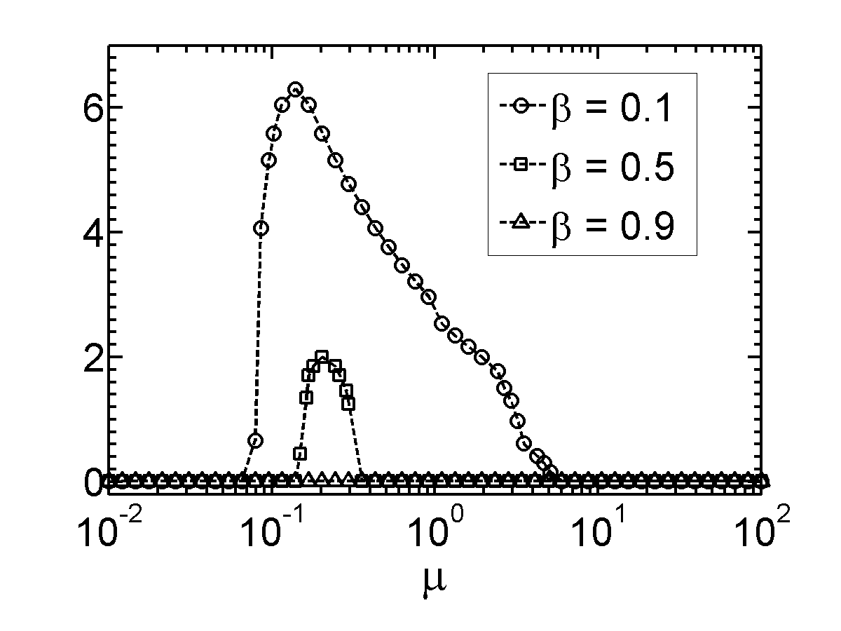
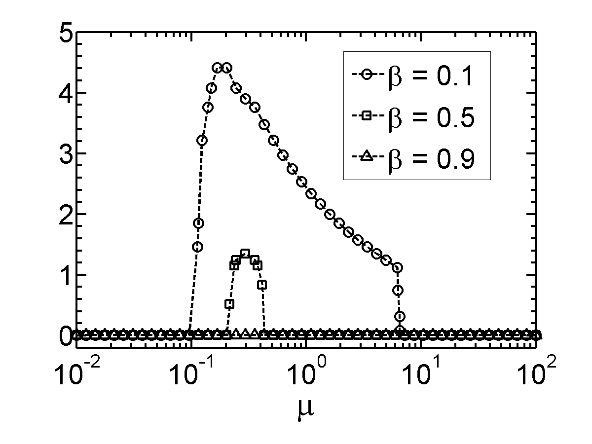
$\bar{\Pi}_{u2}(k_{z},\Omega;\beta,\mu)$	$\bar{\Pi}_{u3}(k_{z},\Omega;\beta,\mu)$

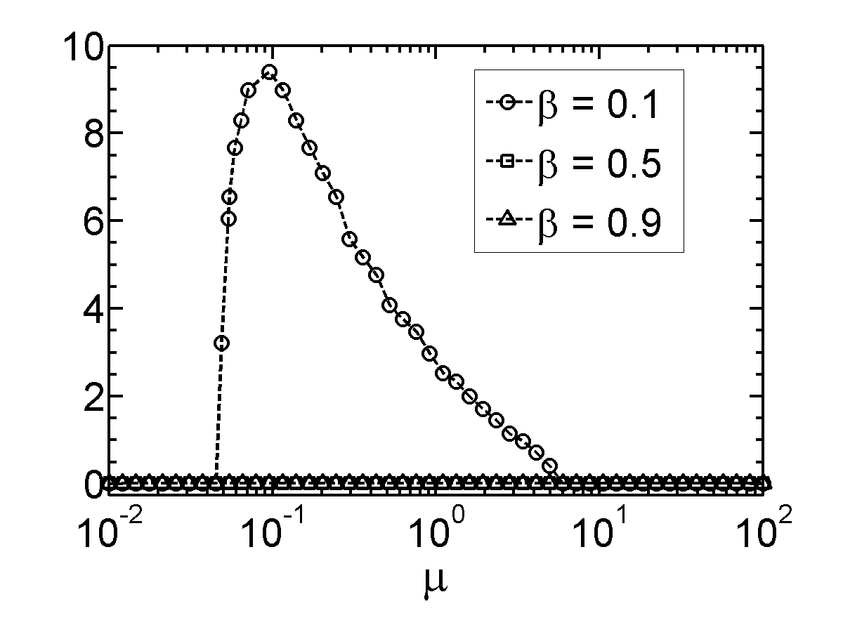
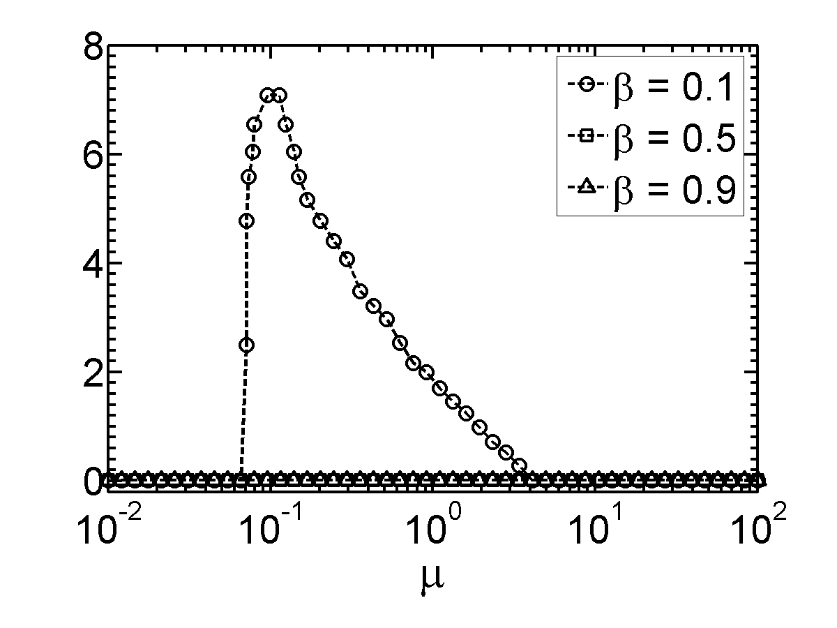
Figure 6: Variation in $\Omega_{\max}$ with $\mu$ for Couette (first row) and Poiseuille (second row) flows with $\beta\,=\,\{0.1$, $0.5$, $0.9\}$.

The analytical expressions for $\Omega_{\max}$ are much more difficult to obtain for the base-flow-dependent power spectral densities $\bar{\Pi}_{u2}$ and $\bar{\Pi}_{u3}$. In spite of this, essential trends can be ascertained from figure 7, which shows the plots of function $\bar{\Pi}_{b}(k_{z},\Omega;\beta,\mu)$ in Couette flow with $\beta\,=\,0.1$ and $\mu\,=\,\{0.1$, $2$, $10$, $100\}$. (This function quantifies the power spectral density of the frequency response operator that maps ($d_{2},d_{3}$) to streamwise velocity $u$ at $Re\,=\,1$.) For $\mu\,=\,0.1$, the frequency response achieves a global maximum at $\Omega_{\max}\,=\,0$, but the broad spectrum in $\Omega$ around $k_{z}\,\approx\,O(1)$ indicates that the large values are maintained up until $\Omega\,\approx\,5$. On the other hand, at $\mu\,=\,2$, the global peak is located in the narrow region around $\Omega_{\max}\,\approx\,2$. With a further increase in elasticity number, two competing peaks at zero and $O(1)$ temporal frequencies appear; finally, for large values of $\mu$ the spectrum peak shifts to the narrow region around zero temporal frequency, with $\Omega_{\max}\,=\,0$.

$\mu\,=\,0.1$	$\mu\,=\,2$
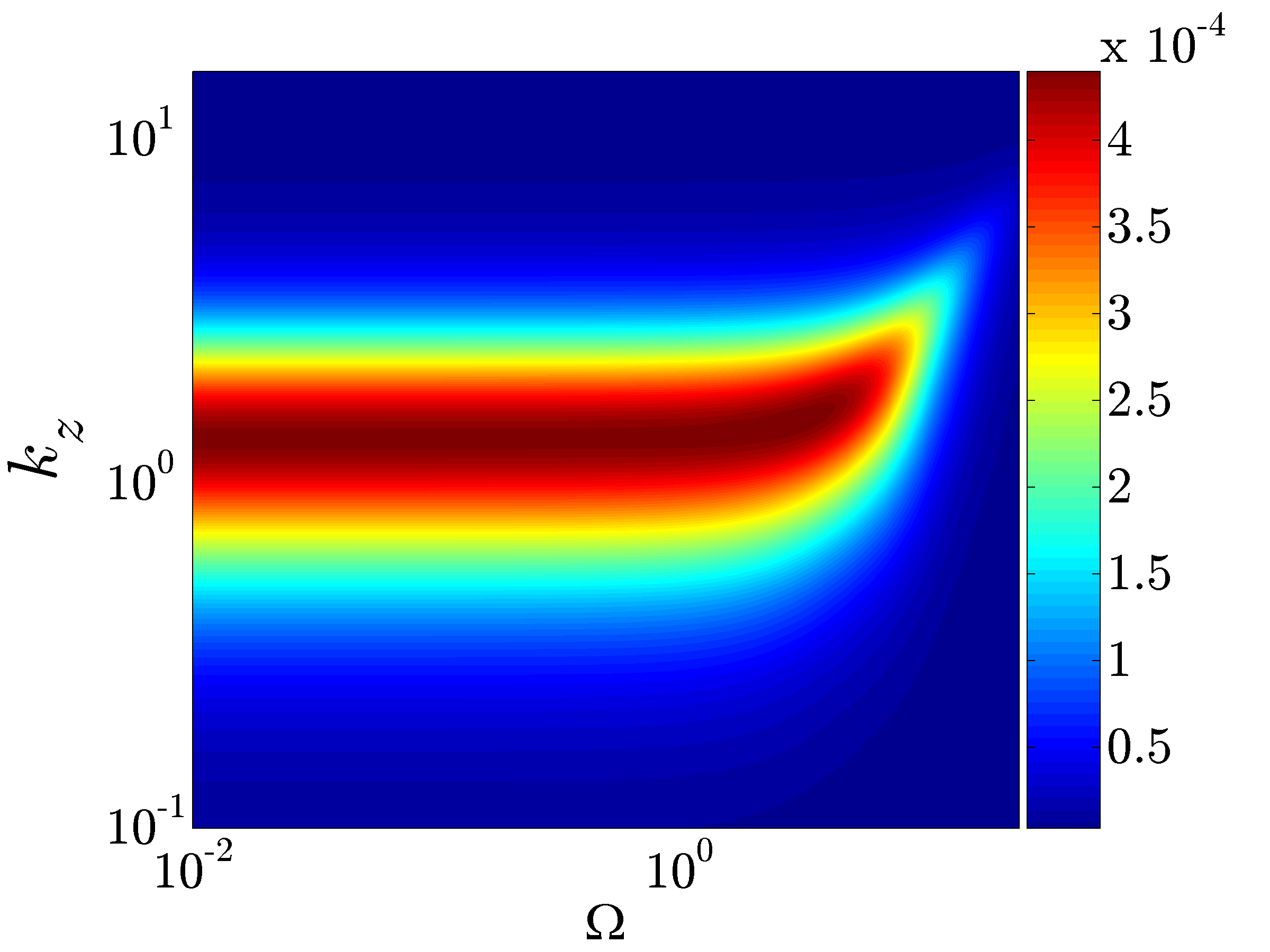
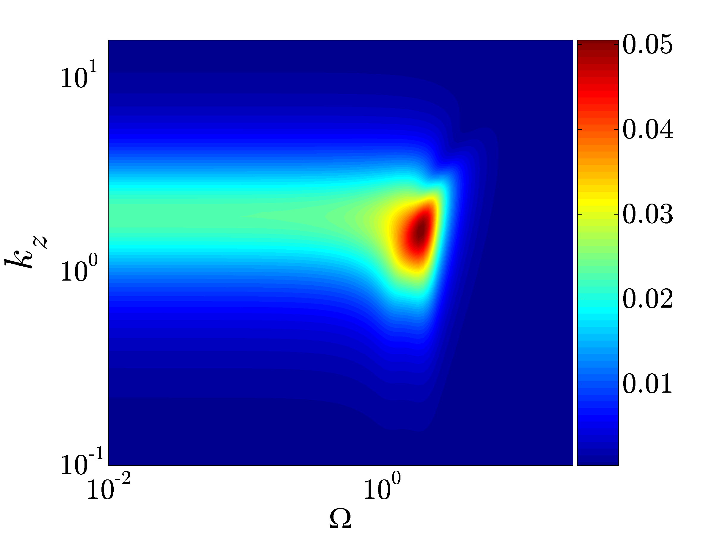
$\mu\,=\,10$	$\mu\,=\,100$

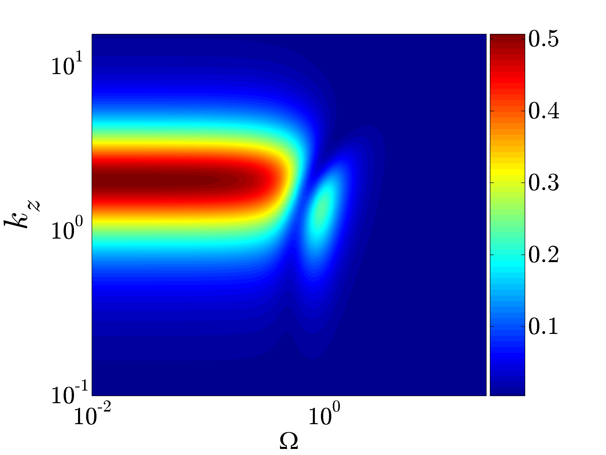
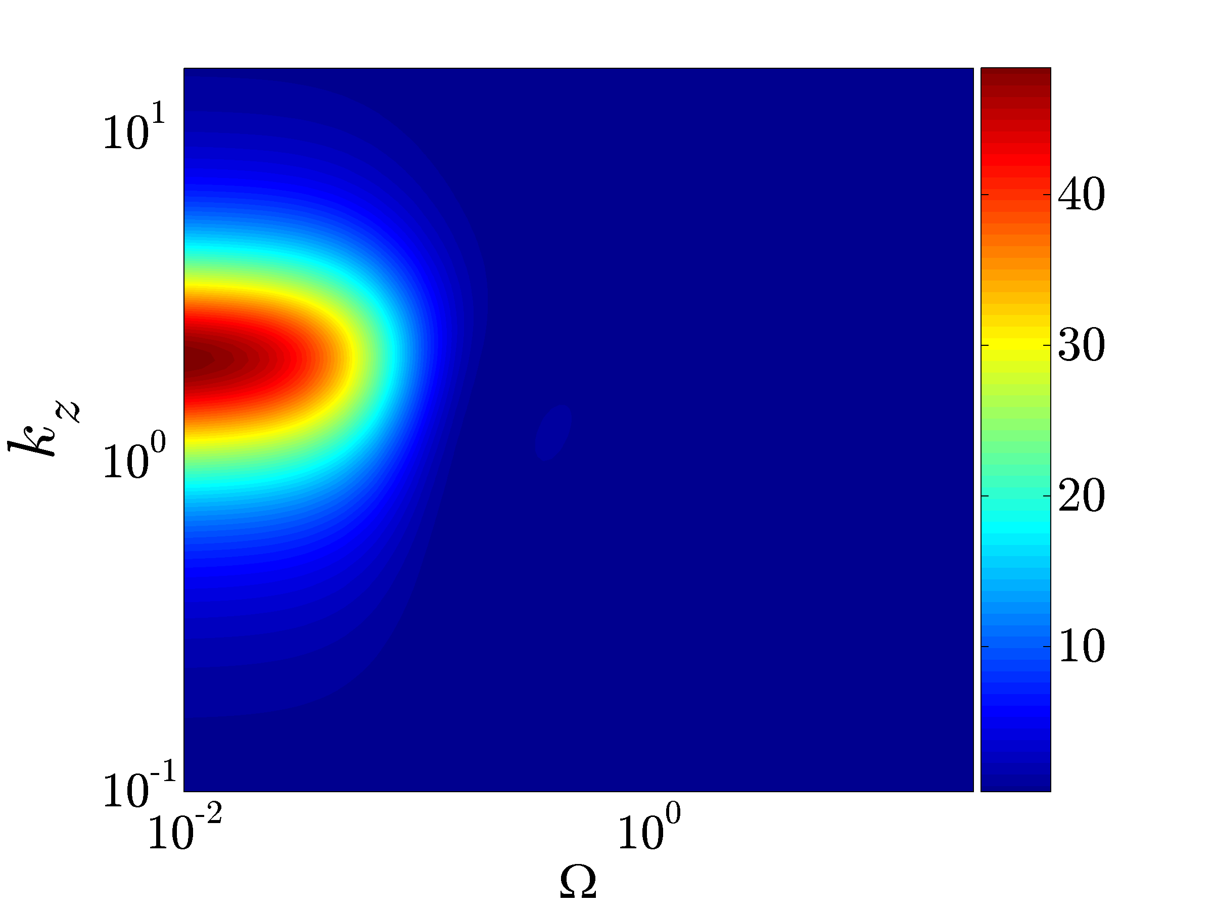
Figure 7: Plots of $\bar{\Pi}_{b}(k_{z},\Omega;\beta,\mu)\,=\,\bar{\Pi}_{u2}(k_{z},\Omega;\beta,\mu)\,+\,\bar{\Pi}_{u3}(k_{z},\Omega;\beta,\mu)$ in Couette flow with $\beta\,=\,0.1$, $\mu\,=\,\{0.1$, $2$, $10$, $100\}$.

We have also studied the effects of $\mu$ and $\beta$ on the maximum value of power spectral densities. We briefly highlight several important points. First, the maximum values of all power spectral densities decrease with an increase in $\beta$ and a decrease in $\mu$. This suggests that amplification becomes weaker as one approaches the Newtonian fluid limit. A similar dependence of the maximum value of the growth function on Deborah (Weissenberg) number was reported by Sureshkumar et al. (1999) in their study of two-dimensional time-dependent simulations of creeping plane Couette flow of Oldroyd-B fluids. Second, the peak values of the base-flow-dependent power spectral densities $\bar{\Pi}_{u2}$ and $\bar{\Pi}_{u3}$ monotonically increase with $\mu$. On the other hand, the peak values of the base-flow-independent power spectral densities $\bar{\Pi}_{u1}$ and $\bar{\Pi}_{rj}$, $\{r=v,w;\;j=2,3\}$, first increase with an increase in $\mu$ and then plateau after $\mu$ becomes sufficiently large. The monotonic increase of $\bar{\Pi}_{u2}$ and $\bar{\Pi}_{u3}$ with the elasticity number demonstrates the significance of the coupling operator $\mathbf{C}_{p2}$, which captures the work done by the polymer stresses on the flow. An in-depth study of the physical mechanisms behind this viscoelastic amplification is given in § 6. Third, the spanwise wavenumbers corresponding to the maxima in the components of the frequency response increase with an increase in $\mu$ and a decrease in $\beta$. This suggests that the dominant structures become less spread in the spanwise direction with an increase in $\mu$ and a decrease in $\beta$.

6 Energy amplification mechanisms

In order to elucidate the energy amplification mechanisms in Oldroyd-B fluids, we next analyze the Reynolds-Orr equation for streamwise-constant channel flow. As is well known, the Reynolds-Orr equation describes the evolution of the energy of velocity fluctuations around a given base flow condition (Schmid & Henningson, 2001). In our study, the initial conditions on velocity and polymer stress fluctuations are set to zero, but the flow is driven by the spatio-temporal stochastic body forcing ${\bf d}$. This random body forcing generates the velocity field ${\bf v}$ and polymer stresses $\tau$, which are also of stochastic nature Farrell & Ioannou (1993).

The energy-evolution equation is derived by multiplying the Navier-Stokes equations by the velocity vector, followed by integration over the wall-normal direction and ensemble averaging in time. The equations are further simplified using the divergence theorem and the boundary conditions on ${\bf v}$. For streamwise-constant perturbations, the Reynolds-Orr equation for an Oldroyd-B fluid is given by:

$$\begin{array}[]{l}\dfrac{1}{2}\dfrac{\mathrm{d}E}{\mathrm{d}t}\;=\;-\,\dfrac{\beta k_{z}^{2}}{Re}E\;-\;\left<u,U^{\prime}v\right>\;+\;\left<{\bf v},{\bf d}\right>\;+\;\dfrac{\beta}{Re}\left(\left<u,\partial_{yy}u\right>\,+\,\left<v,\partial_{yy}v\right>\,+\,\left<w,\partial_{yy}w\right>\right)\\[8.5359pt] -\,\dfrac{1\,-\,\beta}{Re}\left(\left<\tau_{xy},\partial_{y}u\right>\,+\,\left<\tau_{yz},\partial_{y}v\right>\,+\,\left<\tau_{xz},\partial_{y}w\right>\,+\,\mathrm{i}k_{z}\left(\left<\tau_{xz},u\right>\,+\,\left<\tau_{yz},v\right>\,+\,\left<\tau_{zz},w\right>\right)\right),\end{array}$$

where $\left<\cdot,\cdot\right>$ denotes integration in $y$ and ensemble averaging in $t$, and $E\,=\,E(t,k_{z};Re,\beta,\mu)$ represents the kinetic energy, that is

$$E\;=\;\left<{\bf v},{\bf v}\right>\;=\;\int_{-1}^{1}{\cal E}\left({\bf v}^{*}(y,k_{z},t){\bf v}(y,k_{z},t)\right)\,\mathrm{d}y.$$

Here, the asterisk denotes the complex-conjugate-transpose of vector ${\bf v}$, and ${\cal E}$ denotes ensemble averaging McComb (1991)

$${\cal E}\left({\bf v}(\cdot,t)\right)~{}=~{}\lim_{T\,\rightarrow\,\infty}\dfrac{1}{T}\int_{0}^{T}{\bf v}(\cdot,t+\tau)\,\mathrm{d}\tau.$$

In the steady-state limit, the kinetic energy $E$ is given by

$$\begin{array}[]{l}E\;=\;\dfrac{Re}{\beta k_{z}^{2}}\left(-\langle u,U^{\prime}v\rangle\;+\;\left<{\bf v},{\bf d}\right>\right)\;+\;\dfrac{1}{k_{z}^{2}}\left(\left<u,\partial_{yy}u\right>\,+\,\left<v,\partial_{yy}v\right>\,+\,\left<w,\partial_{yy}w\right>\right)\\[8.5359pt] -\,\dfrac{1\,-\,\beta}{\beta k_{z}^{2}}\left(\left<\tau_{xy},\partial_{y}u\right>\,+\,\left<\tau_{yz},\partial_{y}v\right>\,+\,\left<\tau_{xz},\partial_{y}w\right>\,+\,\mathrm{i}k_{z}\left(\left<\tau_{xz},u\right>\,+\,\left<\tau_{yz},v\right>\,+\,\left<\tau_{zz},w\right>\right)\right).\end{array}$$

In this equation, the first two terms on the right-hand-side are contributions due to the Reynolds stress and the work done by the body forces; the third group of terms accounts for viscous dissipation, and the last group of terms corresponds to the work done by the polymer stresses on the flow. This last contribution to kinetic energy is – in general – sign indefinite and it is also referred to as an energy-exchange term Doering et al. (2006).

Two points are worth highlighting. First, as in Newtonian fluids Schmid & Henningson (2001), the nonlinear terms do not contribute to the kinetic energy (they are conservative and only redistribute energy between different modes). Thus, the Reynolds-Orr equations for viscoelastic fluids derived using linearized and fully non-linear equations correspond to each other. Second, the steady-state energy $E$ defined here is exactly the same as the ensemble-average energy density defined in Hoda et al. (2008). As a matter of fact, this quantity is precisely determined by the $H_{2}$ norm of a stochastically forced linearized system. Thus, the energy density of the LNSE can be efficiently computed using Lyapunov equations, which circumvents the need for running costly stochastic numerical simulations.

The explicit scaling of the steady-state energy density with $Re$ is given in § 4. Based on this, for asymptotically large times, $E$ can be written as:

$$E(k_{z};Re,\beta,\mu)\;=\;f(k_{z};\beta,\mu)Re\;+\;g(k_{z};\beta,\mu)Re^{3},$$

where functions $f$ and $g$ correspond to the Reynolds-number-independent terms in Eq. (9). This equation suggests that at higher $Re$ values, $g$ is expected to contribute most to the energy, whereas at smaller $Re$ values, $f$ is expected to contribute most to the energy; we will show that the latter observation holds only at moderate values of $\mu$ and $\beta$. From § 4, it follows that only streamwise velocity contributes to $g$; this contribution arises due to amplification from $d_{2}$ and $d_{3}$ to $u$. On the other hand, amplification from $d_{1}$ to $u$ and $(d_{2},d_{3})$ to $(v,w)$ is captured by function $f$. The explicit $Re$-scaling of various terms in the steady-state Reynolds-Orr equation can be obtained by analyzing the Lyapunov equation (see Appendix B); let the overbar designate the velocity and polymer stress fluctuations at $Re=1$, and let $u_{1}$ and $u_{2,3}$ denote the components of $u$ arising due to the action of $d_{1}$ and ($d_{2},d_{3}$), respectively. Then, the $Re$-independent terms $f(k_{z};\beta,\mu)$ and $g(k_{z};\beta,\mu)$ in the expression for the steady-state energy are given by

$$\begin{array}[]{rcl}f&\!\!=\!\!&\dfrac{1}{\beta k_{z}^{2}}\bigg{(}\left<\bar{{\bf v}},{\bf d}\right>\,+\,\beta\left(\left<\bar{u}_{1},\partial_{yy}\bar{u}_{1}\right>\,+\,\left<\bar{v},\partial_{yy}\bar{v}\right>\,+\,\left<\bar{w},\partial_{yy}\bar{w}\right>\right)\,-\,(1-\beta)\big{(}\left<\bar{\tau}_{xy},\partial_{y}\bar{u}_{1}\right>\\[7.11317pt] &\!\!\!\!&+\,\left<\bar{\tau}_{yz},\partial_{y}\bar{v}\right>\,+\,\left<\bar{\tau}_{xz},\partial_{y}\bar{w}\right>\,+\,\mathrm{i}k_{z}\left(\left<\bar{\tau}_{xz},\bar{u}_{1}\right>\,+\,\left<\bar{\tau}_{yz},\bar{v}\right>\,+\,\left<\bar{\tau}_{zz},\bar{w}\right>\right)\big{)}\bigg{)},\\[7.11317pt] g&\!\!=\!\!&\dfrac{1}{\beta k_{z}^{2}}\left(-\left<\bar{u},U^{\prime}\bar{v}\right>\,+\,\beta\left<\bar{u}_{2,3},\partial_{yy}\bar{u}_{2,3}\right>\,-\,(1\,-\,\beta)\left(\left<\bar{\tau}_{xy},\partial_{y}\bar{u}_{2,3}\right>\,+\,\mathrm{i}k_{z}\left<\bar{\tau}_{xz},\bar{u}_{2,3}\right>\right)\right)\\[7.11317pt] &\!\!=\!\!&g_{\left<u,U^{\prime}v\right>}\,+\,g_{\left<u,\partial_{yy}u\right>}\,+\,g_{\left<\tau_{xy},\partial_{y}u\right>}\,+\,g_{\left<\tau_{xz},\mathrm{i}k_{z}u\right>}.\end{array}$$

We note that function $f$ is the same for all channel flows and only function $g$ depends on the underlying base flow; for further analysis of function $g$, we restrict our attention to Couette flow. Unless noted otherwise, all plots in this section are given in the log-log scale. Figures 8 and 9 show the variations in $f$ and $g$ with $k_{z}$ at different $\beta$ and $\mu$ values. Below, we discuss the important observations concerning the results.

We note that the magnitudes of both $f$ and $g$ increase with an increase in $\mu$ and a decrease in $\beta$. This indicates that energy amplification becomes weaker as one approaches the Newtonian fluid limit. Furthermore, in all the cases, $f$ monotonically decreases with $k_{z}$, while $g$ achieves a maximum at $O(1)$ values of $k_{z}$. This suggests that the contribution from $g$ is responsible for the energy density peaks observed at higher Reynolds numbers Hoda et al. (2008), confirming our earlier claim that at higher $Re$, $E\,\approx\,gRe^{3}$.

Plots in figure 9 suggest that $g$ increases monotonically with $\mu$, while $f$ reaches a saturation limit for sufficiently large values of $\mu$. Thus, even in low inertial regimes, the contribution of $g$ to the energy density can be significant if the elasticity number, $\mu$, is large enough. In particular, this demonstrates that energy density peaks observed by Hoda et al. (2008) at $\{k_{x}=0$, $Re=0.1$, $\beta=0.1$, $\mu=10^{6}\}$ arise due to the contribution of $g$.

Moreover, function $g$ approximately scales linearly with $\mu$ for large values of elasticity number. Figure 9 shows the $k_{z}$-dependence of $g(k_{z};\beta,\mu)/\mu$ in Couette flow with $\beta=0.1$ for five different values of the elasticity number, $\mu\,=\,\{0.1$, $1$, $10$, $10^{2}$, $10^{6}\}$. It is evident that the five curves almost collapse onto each other. This is a remarkable discovery in view of rather complicated dependence of the underlying equations on $\mu$ and the range of elasticity numbers considered. Our ongoing theoretical effort is directed towards development of an explicit scaling of $f$ and $g$ with $\mu$; we conjecture that – for large enough values of elasticity number – $f$ approximately becomes $\mu$-independent, while $g$ approximately scales linearly with $\mu$. This would suggest the following approximate scaling of the energy density with elasticity number for $\mu\,\gg\,1$, $E(k_{z};Re,\beta,\mu)\,\approx\,Re\tilde{f}(k_{z};\beta)\,+\,\mu Re^{3}\tilde{g}(k_{z};\beta)$, where $\tilde{f}$ and $\tilde{g}$ are $\mu$-independent functions. If this scaling turns out to be correct, our results would indicate an interesting interplay between inertial and viscoelastic effects in energy amplification of Oldroyd-B fluids with low Reynolds/high elasticity numbers (Larson, 2000; Groisman & Steinberg, 2000).

$f(k_{z};\beta,\mu)$	$g(k_{z};\beta,\mu)$

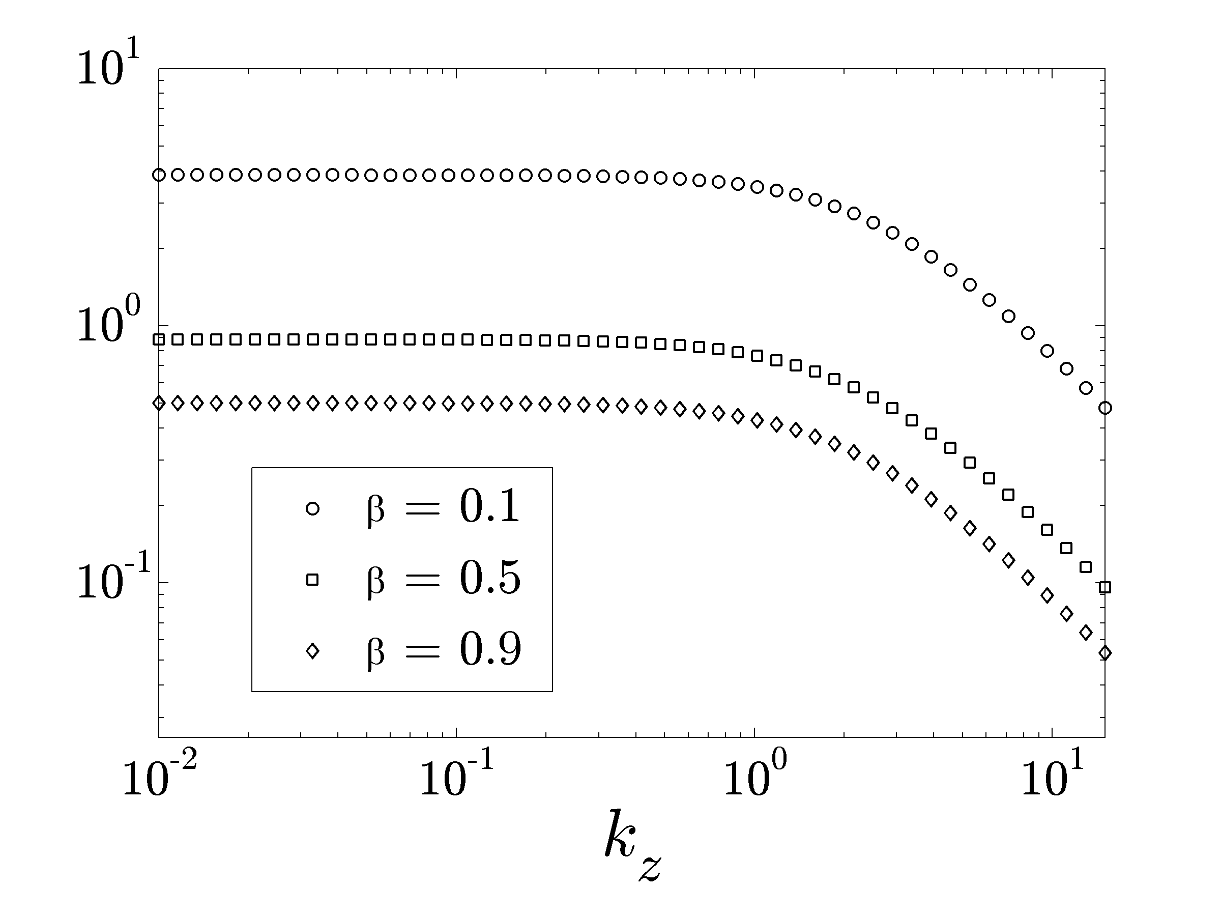
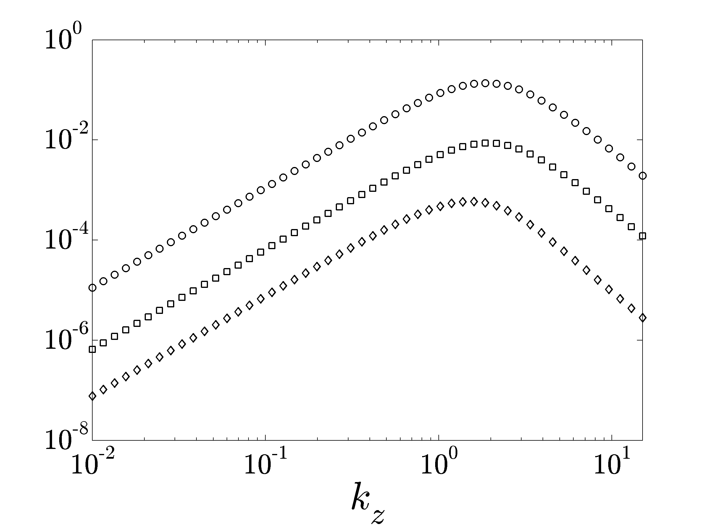
Figure 8: Variation in $f$ and $g$ with $k_{z}$ for $\mu\,=\,10$ and $\beta\,=\,\{0.1$, $0.5$, $0.9\}$; $g$ in Couette flow is shown.

$f(k_{z};\beta,\mu)$	$g(k_{z};\beta,\mu)$	$g(k_{z};\beta,\mu)/\mu$

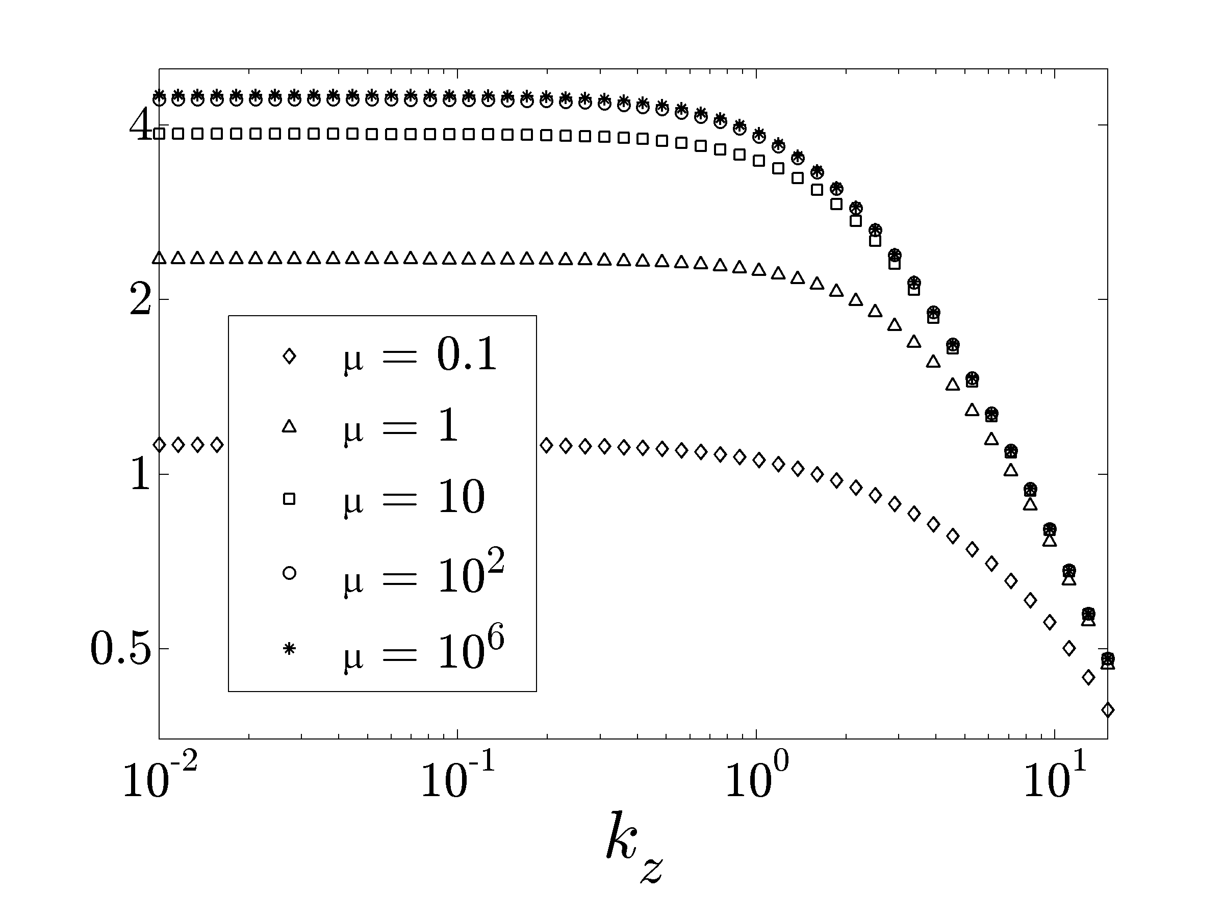
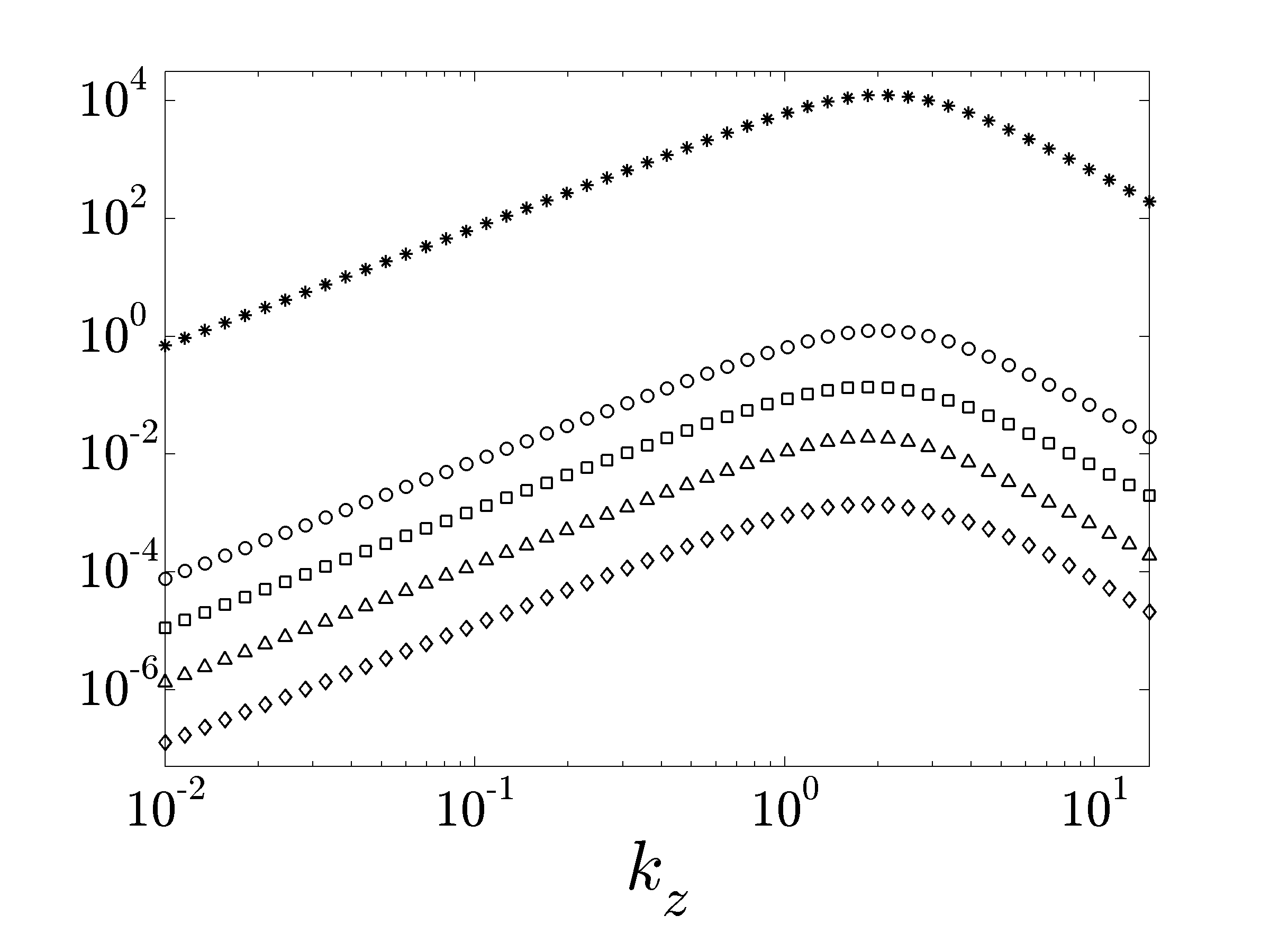
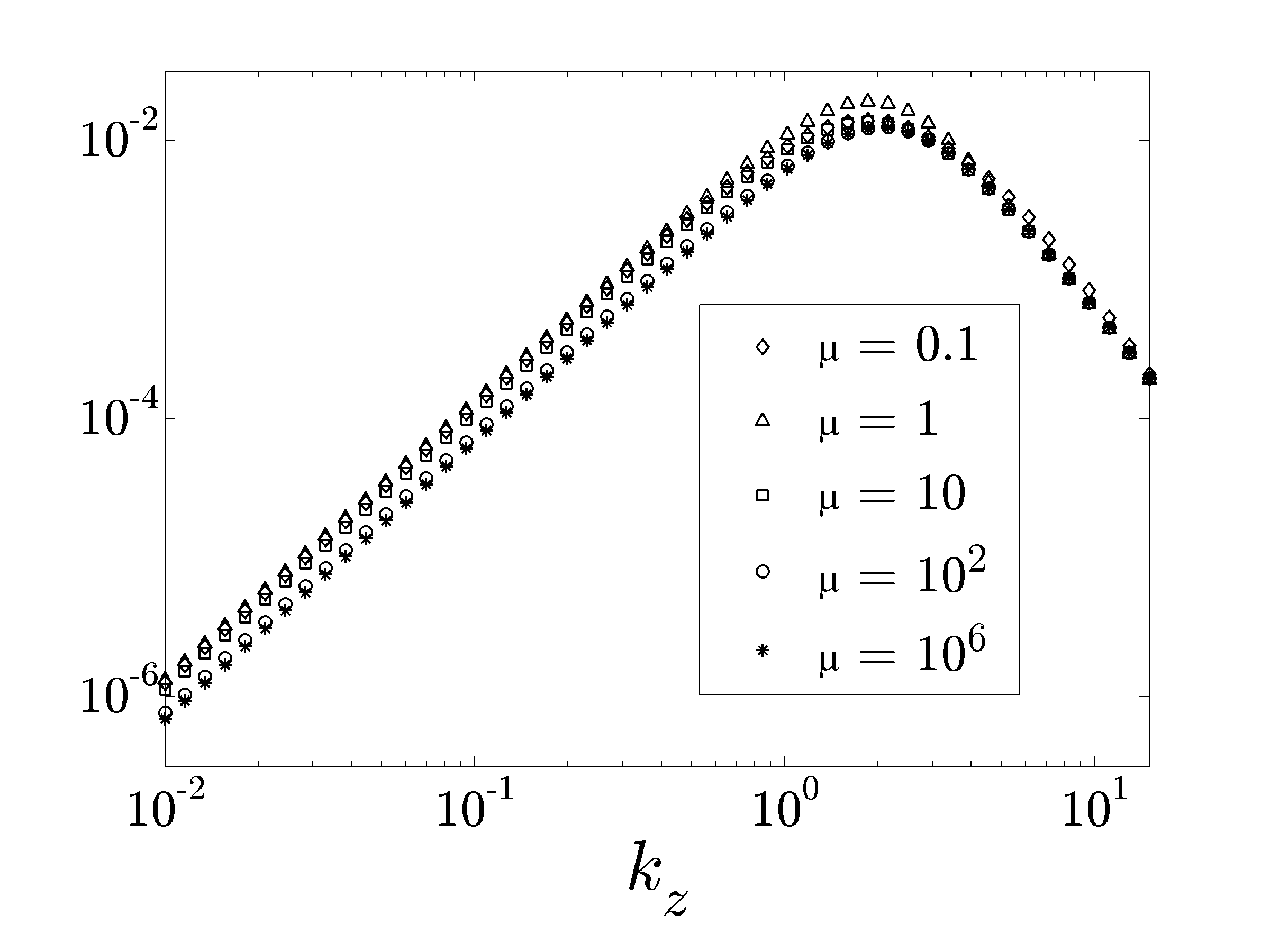
Figure 9: Variation in $f$, $g$, and $g/\mu$ with $k_{z}$ for $\beta\,=\,0.1$ and $\mu\,=\,\{0.1$, $1$, $10$, $10^{2}$, $10^{6}\}$; $g$ in Couette flow is shown.

We have also closely examined the terms in the steady-state Reynolds-Orr equation that contribute to the $Re^{3}$-scaling of energy (results not shown; for details see Hoda (2008)). We observed that the Reynolds-stress and the energy-exchange terms, $g_{\left<u,U^{\prime}v\right>}$ and $g_{\left<\tau_{xy},\partial_{y}u\right>}$, are positive, suggesting that they lead to energy amplification; the viscous dissipation and the energy-exchange terms, $g_{\left<u,\partial_{yy}u\right>}$ and $g_{\left<\tau_{xz},\mathrm{i}k_{z}u\right>}$, are negative, suggesting that they lead to energy suppression. Furthermore, the absolute values of all the terms contributing to $g$ increase with an increase in $\mu$ and a decrease in $\beta$. The Reynolds stress term, $g_{\left<u,U^{\prime}v\right>}$, appears to reach a saturation limit for sufficiently large $\mu$, while there does not appear to be any upper bound on the absolute values of the other terms contributing to $Re^{3}$-scaling as $\mu$ increases. In view of this, we conclude that the energy-exchange terms are mainly responsible for energy amplification in flows with pronounced elasticity effects.

Figure 10 shows the $k_{z}$-dependence of the energy-exchange term $g_{\left<\tau_{xy},\partial_{y}u\right>}$ $+$ $g_{\left<\tau_{xz},\mathrm{i}k_{z}u\right>}$ in Couette flow with $\beta=0.1$ and $\mu=\{0.1$, $1$, $10$, $10^{2}$, $10^{6}\}$. This term contributes to the $Re^{3}$-scaling of the steady-state energy and it can lead to energy suppression (for small $\mu$) or energy amplification (for large $\mu$). Also, the left plot illustrates the sign-indefiniteness of the energy-exchange term for moderate values of $\mu$. Clearly, the role of the energy-exchange term becomes more prominent with increase in elasticity number; in particular, for $\mu\gg 1$ this term creates a much larger contribution to the energy amplification than the Reynolds stress term.

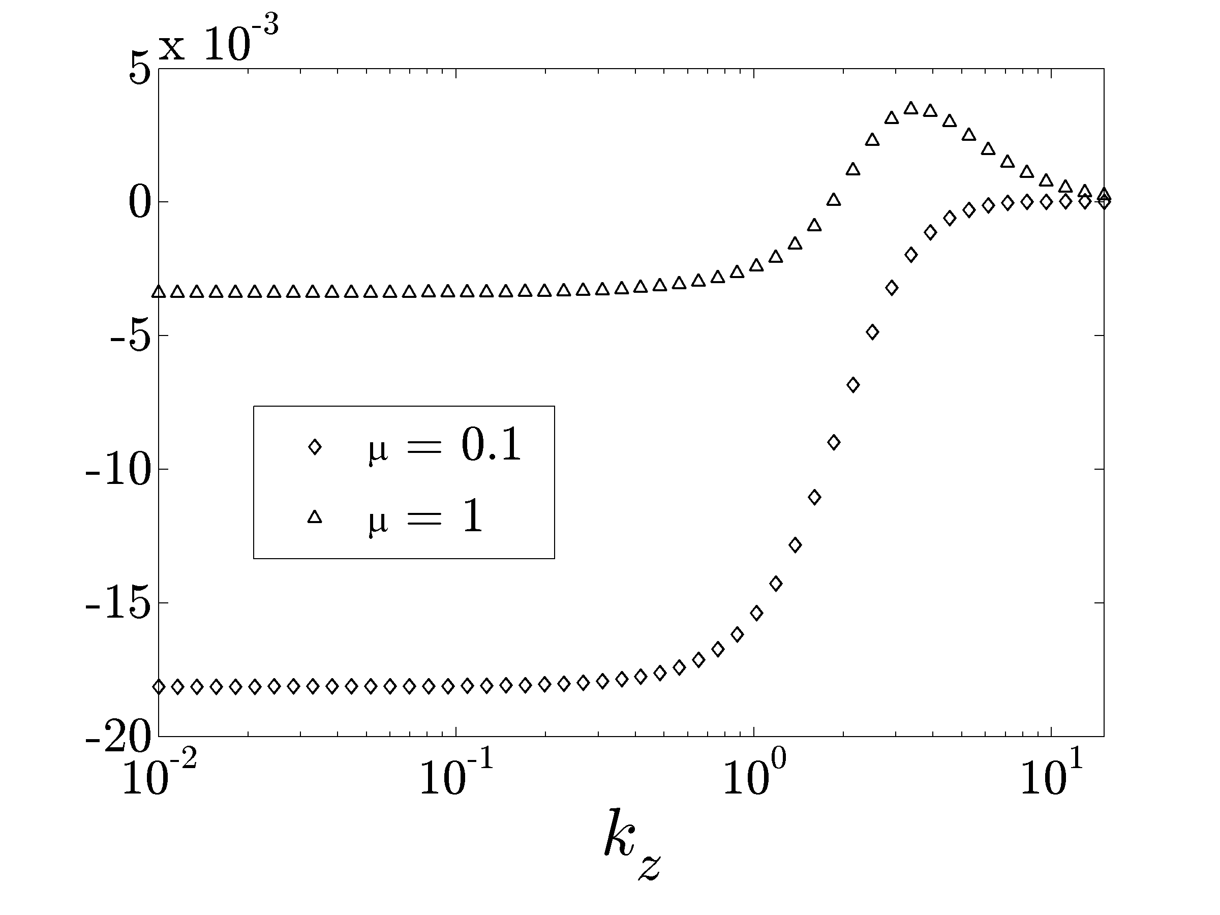
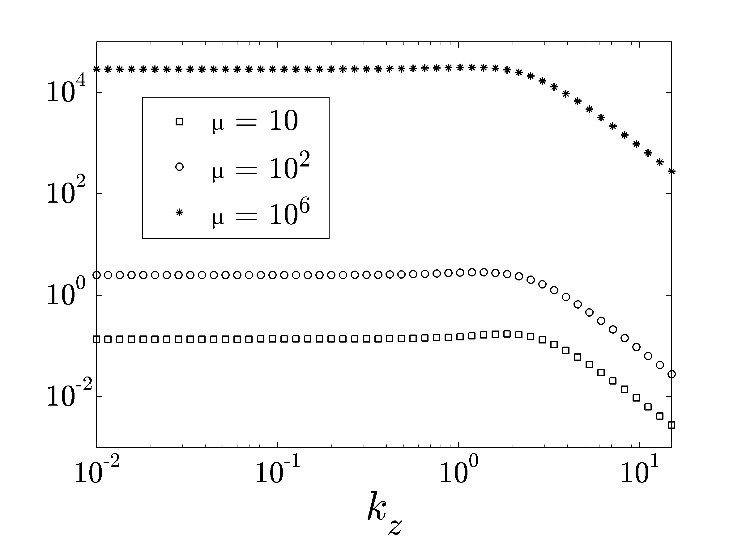
Figure 10: The $k_{z}$-dependence of the energy-exchange term $g_{\left<\tau_{xy},\partial_{y}u\right>}\,+\,g_{\left<\tau_{xz},\mathrm{i}k_{z}u\right>}$ in Couette flow with $\beta=0.1$, $\mu=\{0.1$, $1$, $10$, $10^{2}$, $10^{6}\}$. The left plot is shown in the log-linear scale and the right plot is shown in the log-log scale.

It is interesting to contrast the above results with those of Sadanandan & Sureshkumar (2002), who studied budgets of the perturbation vorticity and kinetic energy in plane Poiseuille flow of Oldroyd-B fluids. Their analysis made use of the linearized equations and a normal-mode decomposition, and considered two-dimensional perturbations. They observed that the temporal frequency near the critical conditions is a non-monotonic function of viscosity ratio, and that perturbation shear stresses have a destabilizing effect. In our work, which does not use a normal-mode decomposition and considers three-dimensional streamwise constant perturbations, $\Omega_{\max}$ is observed to be a monotonic function of $\beta$ (but a non-monotonic function of $\mu$), and perturbation shear stresses are found to create larger energy amplification. We ascribe the differences in these observations to the different assumptions used in the two studies.

Finally, we briefly comment on the terms that contribute to the $Re$-scaling of energy. Apart from work done by the body forces and $-(1-\beta)/(\beta k_{z}^{2})\left<\tau_{yz},\partial_{y}w\right>$, all other terms contributing to $f$ are negative, which suggests that they suppress energy amplification; the most dominant of these terms are $\left<w,\partial_{yy}w\right>$, $\left<u_{1},\partial_{yy}u_{1}\right>$, and $\left<\tau_{xy},\partial_{y}u_{1}\right>$. The absolute values of all the terms, except for the work done by the body forces – which is independent of both $\beta$ and $\mu$ – decrease with an increase in $\beta$. However, the dependence on $\mu$ is more subtle. The absolute values of the viscous-dissipation terms contributing to $f$ increase with an increase in $\mu$, whereas the absolute values of all other terms decrease. The most striking observation is that the absolute values of both $\left<\tau_{xy},\partial_{y}u_{1}\right>$ and $\left<\tau_{xz},\mathrm{i}k_{z}u_{1}\right>$ decrease with an increase in $\mu$, whereas the absolute values of $\left<\tau_{xy},\partial_{y}u_{2,3}\right>$ and $\left<\tau_{xz},\mathrm{i}k_{z}u_{2,3}\right>$ increase with an increase in $\mu$, suggesting competing effects of these energy-exchange terms at $Re=1$.

7 Conclusions

We have investigated the frequency responses of channel flows of Oldroyd-B fluids. Our analysis is based on the 2D/3C model, which simply means that only streamwise-constant perturbations around base values are considered. The disturbances enter the linearized governing equations as a body force that can vary in space and time. The frequency responses are described by an operator having nine blocks, with a given block relating the component $r$ of the velocity perturbation to the disturbance in direction $j$. Characterization of the frequency responses can be performed through calculation of the Hilbert-Schmidt and $H_{2}$ norms; physical interpretations of each of these were discussed.

Our analysis shows that the frequency responses for channel flows of Oldroyd-B fluids scale with the Reynolds number in exactly the same way as in Newtonian fluids. Examination of the associated block diagram reveals that the frequency responses of the spanwise and wall-normal disturbances to streamwise velocity scale as $Re^{2}$, whereas all other frequency responses scale linearly with $Re$. It is also seen that streamwise disturbances do not affect the wall-normal and spanwise velocities. These results indicate that at high Reynolds numbers, channel flows of both Newtonian and viscoelastic fluids are most sensitive to spanwise and wall-normal disturbances, and these disturbances have the largest effect on the streamwise velocity. This is also reflected in the behavior of the various norms, which have the same scalings with $Re$ as is seen for Newtonian fluids. The presence of viscoelasticity causes the frequency responses and their norms to depend on two additional parameters: the elasticity number and viscosity ratio.

A parametric study of the Hilbert-Schmidt norms, or power spectral densities, shows that these peak at non-zero temporal frequencies for viscoelastic fluids. For Newtonian fluids, the peaks occur at zero frequency, indicating that viscoelasticity reduces the time scales over which disturbances develop. The frequencies at which the peaks occur decrease as the solvent contribution to the total viscosity increases, and the peaks are only present if the elasticity number is greater than a critical value. An analytical expression which was derived describes both of these trends accurately. The peak values of the power spectral densities and the corresponding spanwise wavenumbers increase with an increase in elasticity number and a decrease in viscosity ratio. This indicates that elasticity helps amplify spanwise-dependent disturbances and reduces their length scale.

Since each component of the frequency response has its own peak in the Hilbert–Schmidt and $H_{2}$ norms, different amplification mechanisms may occur in a given flow. The componentwise analysis used in the present work makes it easy to detect this, whereas the aggregate analysis used in our previous work does not Hoda et al. (2008). The study of the power spectral and steady-state energy densities also shows that at low Reynolds and elasticity numbers, the flow is most sensitive to streamwise disturbances, and these affect the streamwise velocity the most. At low Reynolds and high elasticity numbers, the flow is most sensitive to wall-normal and spanwise disturbances, and these again affect the streamwise velocity the most.

To elucidate how elasticity amplifies disturbances, we have analyzed a Reynolds-Orr equation for the kinetic energy. Its steady-state value is exactly the same as the $H_{2}$ norm. Our analysis shows that the energy-exchange term involving the polymer stress component $\tau_{xy}$ and the wall-normal gradient of the streamwise velocity $\partial_{y}u$ promotes energy amplification. In contrast, the energy-exchange term involving the polymer stress component $\tau_{xz}$ and the spanwise gradient of the streamwise velocity $\mathrm{i}k_{z}u$ leads to energy suppression. The energy-exchange term that promotes energy amplification becomes increasingly important relative to the Reynolds stress term as the elasticity number increases, and is thus the main driving force for amplification in flows with strong viscoelastic effects.

The results of the present work significantly extend our knowledge of how viscoelastic channel flows respond to external disturbances. They clearly demonstrate how streamwise-constant disturbances can produce significant energy amplification, and clarify the relationship between the components of the disturbances and velocity field. Notably, the results cover both inertia- and elasticity-dominated flows. We expect that they will provide a useful basis for studies exploring nonlinear aspects of transition to inertial and/or elastic turbulence in channel flows of viscoelastic fluids. It might also be possible to extend the ideas developed here to study interfacial instabilities, where the linearized governing equations are also non-normal in nature Lin, Khomami & Sureshkumar (2004).

Appendix A Frequency response operators

The Reynolds-number-independent frequency response operators $\bar{\mathbf{H}}_{rj}$ can be obtained by applying the temporal Fourier transform to Eqs. (3). Equation (3b) can be used to express polymer stresses $\mbox{\boldmath$\phi$}_{2}\,=\,\left[\,\tau_{yy}~{}\tau_{yz}~{}\tau_{zz}\,\right]^{T}$ in terms of wall-normal velocity $\phi_{1}\,=\,v$

$$\mbox{\boldmath$\phi$}_{2}\;=\;\dfrac{\mathbf{F}_{21}}{1\,+\,\mathrm{i}\mu\Omega}\phi_{1},~{}~{}~{}\Omega\;=\;\omega Re.$$ (10)

Substitution of Eq. (10) into the Fourier transform of Eq. (3a) yields

$$\phi_{1}\;=\;Re\left(\mathrm{i}\Omega\mathbf{I}\,-\,\beta\mathbf{F}_{11}\,-\,\dfrac{1\,-\,\beta}{1\,+\,\mathrm{i}\mu\Omega}\mathbf{F}_{12}\mathbf{F}_{21}\right)^{-1}\left(\mathbf{B}_{2}d_{2}\,+\,\mathbf{B}_{3}d_{3}\right).$$ (11)

Using Eq. (3n) and the fact that $\mathbf{F}_{12}\mathbf{F}_{21}\,=\,\mathbf{F}_{11}\,=\,\mbox{\boldmath$\Delta$}^{-1}\mbox{\boldmath$\Delta$}^{2}$, the expressions for operators $\bar{\mathbf{H}}_{rj}(k_{z},\Omega;\beta,\mu),$ $\{r=v,w;\;j=2,3\},$ are readily established (cf. § 4).

The following relation between the wall-normal velocity/vorticity ($\phi_{1},\phi_{3}$) and polymer stresses $\mbox{\boldmath$\phi$}_{4}\,=\,\left[\,\tau_{xy}~{}\tau_{xz}\,\right]^{T}$ can be established by substituting Eq. (10) to the Fourier transform of Eq. (3d)

$$\mbox{\boldmath$\phi$}_{4}\;=\;\dfrac{\mu Re}{1\,+\,\mathrm{i}\mu\Omega}\left(\mathbf{F}_{41}\,+\,\dfrac{\mathbf{F}_{42}\mathbf{F}_{21}}{1\,+\,\mathrm{i}\mu\Omega}\right)\phi_{1}\;+\;\dfrac{1}{1\,+\,\mathrm{i}\mu\Omega}\mathbf{F}_{43}\phi_{3}.$$

Substituting the above equation in the Fourier transform of Eq. (3c) yields

$$\begin{array}[]{rcl}\phi_{3}&\!\!=\!\!&Re\left(\mathrm{i}\Omega\mathbf{I}-\beta\mathbf{F}_{33}-\dfrac{(1-\beta)}{1+\mathrm{i}\mu\Omega}\mathbf{F}_{34}\mathbf{F}_{43}\right)^{-1}\left(\mathbf{F}_{31}+\dfrac{\mu(1-\beta)\mathbf{F}_{34}}{1+\mathrm{i}\mu\Omega}\left(\mathbf{F}_{41}+\dfrac{\mathbf{F}_{42}\mathbf{F}_{21}}{1+\mathrm{i}\mu\Omega}\right)\right)\phi_{1}\\[7.11317pt] &\!\!+\!\!&Re\left(\mathrm{i}\Omega\mathbf{I}-\beta\mathbf{F}_{33}-\dfrac{(1-\beta)}{1+\mathrm{i}\mu\Omega}\mathbf{F}_{34}\mathbf{F}_{43}\right)^{-1}\mathbf{B}_{1}d_{1}.\end{array}$$ (12)

Now, since $u\,=\,\mathbf{C}_{u}\phi_{3}$, the expressions for operators $\bar{\mathbf{H}}_{uj}(k_{z},\Omega;\beta,\mu)$, $\{j=1,2,3\}$, given in § 4 follow immediately from this equation and the fact that in Couette and Poiseuille flows we have $\{{\mathbf{F}}_{34}{\mathbf{F}}_{43}={\mathbf{F}}_{33}=\mbox{\boldmath$\Delta$},$ ${\mathbf{F}}_{34}{\mathbf{F}}_{41}=0,$ ${\mathbf{F}}_{34}{\mathbf{F}}_{42}{\mathbf{F}}_{21}=\mathrm{i}k_{z}\left(U^{\prime}(y)\mbox{\boldmath$\Delta$}+2U^{\prime\prime}(y)\partial_{y}\right)\}.$ The latter expression appears in the coupling operator $\mathbf{C}_{p2}$ of § 4. A careful examination of the governing equations shows that this term arises due to the tensor involving polymer stress fluctuations and gradients in the base velocity profile (the $\mbox{\boldmath$\tau$}\cdot\mbox{\boldmath$\nabla$}\mathbf{\overline{v}}$ term in Eq. (1)).

Appendix B Determination of the $H_{2}$ norm using Lyapunov equation

Next, we outline the procedure that is most convenient for determination of the Reynolds-number-independent functions $f$ and $g$ in the expression for the energy amplification. This method exploits the fact that the steady-state energy density of the frequency response operator $\mathbf{H}$ can be determined from the Lyapunov equation, and it is very suitable for uncovering the explicit scaling with $Re$ of various terms in the steady-state Reynolds-Orr equation.

B.1 Lyapunov equation and steady-state energy density

Equations (3a)-(3d) from § 2 can be compactly rewritten as

$$\left[\begin{array}[]{c}\partial_{t}\,\mbox{\boldmath$\varphi$}_{1}\\ \partial_{t}\,\mbox{\boldmath$\varphi$}_{2}\end{array}\right]\;=\;\left[\begin{array}[]{cc}(1/Re)\mathbf{A}_{11}&0\\ \mathbf{A}_{21}&(1/Re)\mathbf{A}_{22}\end{array}\right]\left[\begin{array}[]{c}\mbox{\boldmath$\varphi$}_{1}\\ \mbox{\boldmath$\varphi$}_{2}\end{array}\right]\;+\;\left[\begin{array}[]{c}\mathbf{B}_{11}\\ \mathbf{B}_{21}\end{array}\right]{\bf d},$$

where $\mbox{\boldmath$\varphi$}_{1}=\left[\,\phi_{1}~{}~{}\mbox{\boldmath$\phi$}_{2}^{T}\,\right]^{T}$, $\mbox{\boldmath$\varphi$}_{2}=\left[\,\phi_{3}~{}~{}\mbox{\boldmath$\phi$}_{4}^{T}\,\right]^{T}$, and

$$\begin{array}[]{c}\mathbf{A}_{11}\;=\;\left[\begin{array}[]{cc}\beta\mathbf{F}_{11}&(1-\beta)\mathbf{F}_{12}\\ (1/\mu)\mathbf{F}_{21}&-(1/\mu)\mathbf{I}\end{array}\right],~{}~{}\mathbf{A}_{22}\;=\;\left[\begin{array}[]{cc}\beta\mathbf{F}_{33}&(1-\beta)\mathbf{F}_{34}\\ (1/\mu)\mathbf{F}_{43}&-(1/\mu)\mathbf{I}\end{array}\right],\\[9.95863pt] \mathbf{A}_{21}\;=\;\left[\begin{array}[]{cc}\mathbf{F}_{31}&0\\ \mathbf{F}_{41}&\mathbf{F}_{42}\end{array}\right],~{}~{}\mathbf{B}_{11}\;=\;\left[\begin{array}[]{ccc}0&\mathbf{B}_{2}&\mathbf{B}_{3}\\ 0&0&0\end{array}\right],~{}~{}\mathbf{B}_{21}\;=\;\left[\begin{array}[]{ccc}\mathbf{B}_{1}&0&0\\ 0&0&0\end{array}\right].\end{array}$$

Furthermore, the structure of operators $\mathbf{B}_{11}$ and $\mathbf{B}_{21}$ yields

$$\mathbf{M}\;=\;\left[\begin{array}[]{c}\mathbf{B}_{11}\\ \mathbf{B}_{21}\end{array}\right]\left[\begin{array}[]{cc}\mathbf{B}_{11}^{*}&\mathbf{B}_{21}^{*}\end{array}\right]\;=\;\left[\begin{array}[]{cc}\mathbf{M}_{11}&0\\ 0&\mathbf{M}_{22}\end{array}\right],$$

where the asterisk denotes the adjoint of a given operator. From the definitions of operators $\mathbf{B}_{j}$, $j=1,2,3$, and their respective adjoints Jovanović & Bamieh (2005) we have

$$\mathbf{M}_{11}\,=\,\left[\begin{array}[]{cc}\mathbf{B}_{2}\mathbf{B}_{2}^{*}+\mathbf{B}_{3}\mathbf{B}_{3}^{*}&0\\ 0&0\end{array}\right]\,=\,\left[\begin{array}[]{cc}\mathbf{I}&0\\ 0&0\end{array}\right],~{}~{}\mathbf{M}_{22}\,=\,\left[\begin{array}[]{cc}\mathbf{B}_{1}\mathbf{B}_{1}^{*}&0\\ 0&0\end{array}\right]\,=\,\left[\begin{array}[]{cc}\mathbf{I}&0\\ 0&0\end{array}\right].$$

The partition of operators $\mathbf{M}_{11}$ and $\mathbf{M}_{22}$ is done conformably with the partition of vectors $\mbox{\boldmath$\varphi$}_{1}=\left[\,\phi_{1}~{}~{}\mbox{\boldmath$\phi$}_{2}^{T}\,\right]^{T}$ and $\mbox{\boldmath$\varphi$}_{2}=\left[\,\phi_{3}~{}~{}\mbox{\boldmath$\phi$}_{4}^{T}\,\right]^{T}$, respectively.

The steady-state energy density (that is, the $H_{2}$ norm of operator $\mathbf{H}$) can be expressed in terms of the solution to the following operator Lyapunov equation

$$\mathbf{A}\mathbf{P}\;+\;\mathbf{P}\mathbf{A}^{*}\;=\;-\mathbf{M}$$

as $E(k_{z};Re,\beta,\mu)\,=\,\mathrm{trace}\,(\mathbf{N}\mathbf{P}),$ where $\mathbf{P}$ and $\mathbf{N}$ are $2\times 2$ self-adjoint block operators with the following structure

$$\begin{array}[]{c}\mathbf{P}\;=\;\left[\begin{array}[]{cc}\mathbf{P}_{11}&\mathbf{P}_{21}^{*}\\ \mathbf{P}_{21}&\mathbf{P}_{22}\end{array}\right],~{}~{}\mathbf{N}\;=\;\left[\begin{array}[]{cc}\mathbf{N}_{11}&0\\ 0&\mathbf{N}_{22}\end{array}\right],\\[9.95863pt] \mathbf{N}_{11}\,=\,\left[\begin{array}[]{cc}\mathbf{C}_{v}^{*}\mathbf{C}_{v}+\mathbf{C}_{w}^{*}\mathbf{C}_{w}&0\\ 0&0\end{array}\right]\,=\,\left[\begin{array}[]{cc}\mathbf{I}&0\\ 0&0\end{array}\right],~{}~{}\mathbf{N}_{22}\,=\,\left[\begin{array}[]{cc}\mathbf{C}_{u}^{*}\mathbf{C}_{u}&0\\ 0&0\end{array}\right]\,=\,\left[\begin{array}[]{cc}\mathbf{I}&0\\ 0&0\end{array}\right].\end{array}$$

Using the structure of operators $\mathbf{P}$ and $\mathbf{N}$, it follows that $E(k_{z};Re,\beta,\mu)$ is determined by $E(k_{z};Re,\beta,\mu)\,=\,\mathrm{trace}\,(\mathbf{N}\mathbf{P})\,=\,\mathrm{trace}\,(\mathbf{N}_{11}\mathbf{P}_{11})+\mathrm{trace}\,(\mathbf{N}_{22}\mathbf{P}_{22}).$ The same argument as in Bamieh & Dahleh (2001); Jovanović & Bamieh (2005) can be used to show $\{\mathbf{P}_{11}\,=\,Re\,\mathbf{X},$ $\mathbf{P}_{21}\,=\,Re^{2}\,\mathbf{Y},$ $\mathbf{P}_{22}\,=\,Re\,\mathbf{Z}_{1}\,+\,Re^{3}\,\mathbf{Z}_{2}\},$ where the Reynolds-number-independent operators $\mathbf{X}$, $\mathbf{Y}$, and $\mathbf{Z}$ satisfy the following system of conveniently coupled equations

$$\mathbf{A}_{11}\mathbf{X}\;+\;\mathbf{X}\mathbf{A}_{11}^{*} \;=\;-\mathbf{M}_{11},$$

$$\mathbf{A}_{22}\mathbf{Y}\;+\;\mathbf{Y}\mathbf{A}_{11}^{*} \;=\;-\mathbf{A}_{21}\mathbf{X},$$

$$\mathbf{A}_{22}\mathbf{Z}_{2}\;+\;\mathbf{Z}_{2}\mathbf{A}_{22}^{*} \;=\;-(\mathbf{A}_{21}\mathbf{Y}^{*}\;+\;\mathbf{Y}\mathbf{A}_{21}^{*}),$$

$$\mathbf{A}_{22}\mathbf{Z}_{1}\;+\;\mathbf{Z}_{1}\mathbf{A}_{22}^{*} \;=\;-\mathbf{M}_{22}.$$

Hence,

$$\begin{array}[]{rcl}E(k_{z};Re,\beta,\mu)&=&Re\left(\mathrm{trace}\,(\mathbf{N}_{11}\mathbf{X})\,+\,\mathrm{trace}\,(\mathbf{N}_{22}\mathbf{Z}_{1})\right)\;+\;Re^{3}\,\mathrm{trace}\,(\mathbf{N}_{22}\mathbf{Z}_{2})\\ &=&Re\,f(k_{z};\beta,\mu)\;+\;Re^{3}\,g(k_{z};\beta,\mu),\end{array}$$

which provides an efficient way of computing functions $f$ and $g$ in the expression for the steady-state energy density.

B.2 Lyapunov equation and steady-state Reynolds-Orr equation

We next illustrate how the terms on the right-hand side of the steady-state Reynolds-Orr equation can be obtained from the solution of the Lyapunov equation. This allows us to determine the explicit $Re$-scaling of these terms, which clarifies the importance of different energy amplification mechanisms.

We begin by observing that the solution of Lyapunov equation, $\mathbf{P}$, represents the steady-state correlation operator of $\mbox{\boldmath$\varphi$}=\left[\,\mbox{\boldmath$\varphi$}_{1}^{T}~{}~{}\mbox{\boldmath$\varphi$}_{2}^{T}\,\right]^{T}$, that is

$$\mathbf{P}\;=\;\lim_{t\,\rightarrow\,\infty}{\cal E}\left\{\mbox{\boldmath$\varphi$}(\cdot,t)\otimes\mbox{\boldmath$\varphi$}(\cdot,t)\right\},$$

where $\mbox{\boldmath$\varphi$}\otimes\mbox{\boldmath$\varphi$}$ denotes the tensor product of $\varphi$ with itself. This operator contains all the second-order steady-state statistics of the velocity and polymer stress fields. For example, operator $\mathbf{P}_{22}$ carries information about the steady-state correlation of $\mbox{\boldmath$\varphi$}=\left[\,\omega_{y}~{}~{}\tau_{xy}~{}~{}\tau_{xz}\,\right]^{T}$ with itself, and a simple kinematic relationship between $\omega_{y}$ and $u$ (at $k_{x}=0$, $u=\mathbf{C}_{u}\omega_{y}=-(\mathrm{i}/k_{z})\omega_{y}$) can be used to obtain all possible correlations between $u$, $\tau_{xy}$, and $\tau_{xz}$. In particular, owing to the convenient scaling of $\mathbf{P}_{22}$ with the Reynolds number ($\mathbf{P}_{22}=Re\,\mathbf{Z}_{1}\,+\,Re^{3}\,\mathbf{Z}_{2}$), we conclude that all these correlations contain a part that scales as $Re$ and a part that scales as $Re^{3}$. (The streamwise force is responsible for the $Re$-scaling and the wall-normal and spanwise forces are responsible for the $Re^{3}$-scaling.) Now, since the inner product of two fields is equal to the trace of their outer (tensor) product, we conclude that the terms $\left<u,\partial_{yy}u\right>$, $\left<\tau_{xy},\partial_{y}u\right>$, and $\left<\tau_{xz},\mathrm{i}k_{z}u\right>$ in the steady-state Reynolds-Orr equation scale as $f_{i}(k_{z};\beta,\mu)Re+g_{i}(k_{z};\beta,\mu)Re^{3}$, $\{i=\left<u,\partial_{yy}u\right>$, $\left<\tau_{xy},\partial_{y}u\right>$, $\left<\tau_{xz},\mathrm{i}k_{z}u\right>\}$. Since the Reynolds stress term $-\left<u,U^{\prime}v\right>$ can be determined from $\mathbf{P}_{21}=Re^{2}\mathbf{Y}$, it follows that its contribution to the steady-state energy scales as $Re^{3}$ (cf. § 6). The contributions of all other terms scale as $Re$.