Cross-fertilization of Ferreira’s Hopfions And Electromagnetic Knots

Abstract

The interrelation between Ferreira’s Hopf solitons of a conformal nonlinear $\sigma$ model and the electromagnetic knots found by Ra$\tilde{\rm{n}}$ada et al. is investigated. It is shown that the electromagnetic knots yield exact solutions of the conformal nonlinear $\sigma$ model different from those obtained by Ferreira. Conversely, It is discussed that Ferreira’s solutions realize magnetic knots. The energy associated with these two kinds of knots are compared. The structure of the electric charge distribution and the electric current density associated with the magnetic knots is investigated.

———————————————————————————————

Corresponding author: Chang-Guang Shi, shichangguang@shiep.edu.cn

1 Introduction

Recently, the electromagnetic knots have attracted much attention[1, 2, 3]. They are the solutions of the Maxwell equations in the vacuum possessing knot structures. As every physicist knows, the Maxwell equations in the vacuum are given by

$$\partial_{\mu}F^{\mu\nu}=0,\quad\partial_{\mu}\tilde{F}^{\mu\nu}=0,$$ (1)

where $F_{\mu\nu}$ and $\tilde{F}^{\mu\nu}$ are defined by

$$F_{\mu\nu}=\partial_{\mu}A_{\nu}-\partial_{\nu}A_{\mu},\quad\tilde{F}^{\mu\nu}=\frac{1}{2}\varepsilon^{\mu\nu\alpha\beta}F_{\alpha\beta}$$ (2)

in terms of the $4$-potential $A_{\mu}$. Here $\varepsilon^{\mu\nu\alpha\beta}$ is the totally anti-symmetric Levi-Civita tensor. They might be important in plasma physics and fluid dynamics. Besides theoretical interests, it was discussed that the electromagnetic knots might be the origin of the phenomenon of ball lightning[4, 5, 6].
On the other hand, Ferreira[7] succeeded in obtaining the $3+1$ dimensional solutions of a model, which we refer to as the conformal nonlinear $\sigma$ model (CNLSM) in this paper, for a complex scalar field. It is expected that the CNLSM has connections to the low energy limit of the Yang-Mills theory and the Skyrme-Faddeev model[8, 9].
Because of the conformal symmetry of the electromagnetism and the CNLSM, the solutions of both theories can involve a parameter specifying the space-time scale and the energies associated with these solutions are proportional to the inverse of this scale parameter. Therefore they cannot be energetically-stable configurations. The solutions of both theories, however, can be topologically-stable in the sense that conserved topological numbers can be defined for them.
Two Hopf indices are defined for an electromagnetic knot, while a single Hopf index is defined for a solution of the CNLSM.
The Lagrangian density of the CNLSM is given by[7]

$$\mathcal{L}_{F}=-\frac{1}{4}H_{\mu\nu}H^{\mu\nu},$$ (3)

where $H_{\mu\nu}$ is defined by

$$H_{\mu\nu}=\frac{1}{2}\bm{n}\cdot(\partial_{\mu}\bm{n}\times\partial_{\nu}\bm{n})=\frac{1}{i}\frac{(\partial_{\mu}u\partial_{\nu}u^{*}-\partial_{\nu}u\partial_{\mu}u^{*})}{(1+uu^{*})^{2}}.$$ (4)

Here $\bm{n}$ denotes a point on $S^{2}$

$$\bm{n}=\left(n^{1},n^{2},n^{3}\right),\quad{\bm{n}}^{2}=\bm{n}\cdot\bm{n}=\sum\limits_{a=1}^{3}n^{a}n^{a}=1$$ (5)

which is related to the complex field $u$ by the stereographic projection

$$\bm{n}=\frac{1}{1+uu^{*}}\left(u+u^{*},-i(u-u^{*}),uu^{*}-1\right)\quad{\rm{or}}\quad u=\frac{n_{1}+in_{2}}{1-n_{3}}.$$ (6)

Regarding $u$ and $u^{*}$ as the fundamental fields, the field equations are given by

$$\partial_{\mu}\left(H^{\mu\nu}\partial_{\nu}u\right)=0,\quad\partial_{\mu}\left(H^{\mu\nu}\partial_{\nu}u^{*}\right)=0.$$ (7)

In this paper, we discuss that these two theories can cross-fertilise each other. We show that the electromagnetic configurations discussed in the theory of electromagnetic knots supplies us with a new class of solutions of the CNLSM different from those obtained by Ferreira.

Conversely, we show also that Ferreira’s solution of the CNLSM, which we hereafter refer to as F-Hopfions, supplies us with a class of exact magnetic knot configurations in some electric charge and current distributions. We investigate the electric field, magnetic field, electromagnetic energy, electric charge density and the electric current density which arise from F-Hopfions. If we adopt the same scale parameter in the simplest nontrivial examples of the two theories, it turns out that the energy of the electromagnetic field obtained from F-Hopfion is equal to the half of that of the configuration discussed in the theory of electromagnetic knot.

This paper is organized as follows. In Sec.2, we first discuss that F-Hopfions are the $3+1$-dimensional generalizations of the Hopf fibration. We then compare the simplest F-Hopfion with the configuration of the complex scalar fields appearing in the electromagnetic knots. We next obtain new solutions of the CNLSM which are different from F-Hopfions. In Sect.3, we investigate the electromagnetism implied by F-Hopfions. It corresponds to the electromagnetism not in the vacuum but in non-vanishing electric charge and current distributions. We discuss some properties of them. The final section is devoted to summary.

2 F-Hopfion and Hopf fibration

Guided by the invariance of CNLSM under the conformal group $SO(4,2)$ of the four-dimensional Minkowski space-time[10], the following variables $Y,\zeta,\varphi$ and $\xi$ are introduced in [7]. Expressing $(x^{0},x^{1},x^{2},x^{3})$ as $(t,x,y,z)$, they are defined by

$$\displaystyle{t=\frac{a}{p}\sin\zeta,\quad x=\frac{a}{p}\frac{\cos\varphi}{\sqrt{1+Y}}},\quad\displaystyle{y=\frac{a}{p}\frac{\sin\varphi}{\sqrt{1+Y}}},\quad\displaystyle{z=\frac{a}{p}\sin\xi\sqrt{\frac{Y}{1+Y}}},$$

$$\displaystyle{p=\cos\zeta-\cos\xi\sqrt{\frac{Y}{1+Y}},}$$ (8)

where $a$ is an arbitrary constant parameter of the dimension of length which fixes the space-time scale. For simplicity we hereafter set $a=1$. Then we have

$$\displaystyle{Y=\frac{\left(1+s^{2}\right)^{2}+4z^{2}}{4\rho^{2}},\quad\tan\varphi=\frac{y}{x}},\quad\displaystyle{\tan\zeta=\frac{2t}{1-s^{2}}},\quad\displaystyle{\tan\xi=-\frac{2z}{1+s^{2}}.}$$

$$\displaystyle{s^{2}=t^{2}-r^{2},\quad r^{2}=\rho^{2}+z^{2},\quad\rho^{2}=x^{2}+y^{2}.}$$ (9)

It is striking that the Ansatz

$$u=\sqrt{\frac{1-g}{g}}{\rm{e}}^{i\Phi},\quad g=g(Y),\quad\Phi=\Phi(\xi,\varphi,\zeta)=m_{1}\xi+m_{2}\varphi+m_{3}\zeta,$$ (10)

with $m_{1},m_{2},m_{3}$ being integers and $m_{1}+m_{2}+m_{3}$ being an even integer is compatible with the field equation and the single-valuedness of $u$ [7].
Under the Ansatz (10), the field equation (7) is reduced to a linear ordinary differential equation

$$\frac{d}{dY}\left(\Lambda\frac{dg}{dY}\right)=0,\quad\Lambda=m_{1}^{2}(1+Y)+m_{2}^{2}Y(1+Y)-m_{3}^{2}Y.$$ (11)

The solutions of this equation can be classified by the parameters $\Delta$ and $b$ defined by $\Delta=\frac{1}{4m_{2}^{2}}\left[(m_{1}+m_{3})^{2}-m_{2}^{2}\right]\left[(m_{1}-m_{3})^{2}-m_{2}^{2}\right],b=\frac{m_{1}^{2}+m_{2}^{2}-m_{3}^{2}}{2m_{2}^{2}}$ and the Hopf index of the solution was calculated to be $Q_{H}=m_{1}m_{2}[g(0)-g(\infty)]$ [7].

We first discuss the simplest nontrivial case ($m_{1}=m_{2}=1,~{}m_{3}=0$) briefly. In this case, the field equation becomes $\frac{d}{dY}\left[(Y+1)^{2}\frac{dg}{dY}\right]=0$. If we adopt the boundary condition $g(0)=0,g(\infty)=1$, we obtain $g(Y)=\frac{Y}{Y+1}$, from which we have

$$u=\frac{{\rm{e}}^{i(\xi+\varphi)}}{\sqrt{Y}}.$$ (12)

We then find

$$u=i\phi_{H}\quad{\rm{at}}\quad t=0,$$ (13)

where $\phi_{H}$ is the Hopf fibration

$$\phi_{H}=\frac{2(x+iy)}{2z+i(r^{2}-1)}.$$ (14)

In other words, the simplest example of F-Hopfion is a $3+1$-dimensional generalization of the Hopf fibration. We note that the Hopf index of the above $u$ is equal to $-1$.
The $3+1$-dimensional generalizations of $\phi_{H}$ different from the above $u$ are given by [2, 3, 4, 6]

$$\displaystyle{\eta_{m}=-\frac{[Ky+t(K-1)]+i(tz-Kx)}{(Kz+tx)+i[K(K-1)-ty]}},$$

$$\displaystyle{\eta_{e}=i\frac{(Kz+tx)+i[Ky+t(K-1)]}{(tz-Kx)+i[K(K-1)-ty]},}$$

$$K\displaystyle{\equiv\frac{1}{2}(1-s^{2})=\frac{1}{2}(r^{2}-t^{2}+1)}.$$ (15)

Although we can introduce the scale parameter $a$ similarly to the case of F-Hopfion, we consider the case of $a=1$ again for simplicity. The remarkable property of the pair ($\eta_{e}$, $\eta_{m}$) is that they satisfy

$$\displaystyle{\frac{1}{i(1+\eta_{m}\eta_{m}^{*})^{2}}\frac{\partial(\eta_{m},\eta_{m}^{*})}{\partial(y,z)}=\frac{1}{i(1+\eta_{e}\eta_{e}^{*})^{2}}\frac{\partial(\eta_{e},\eta_{e}^{*})}{\partial(t,x)},}$$

$$\displaystyle{\frac{1}{i(1+\eta_{e}\eta_{e}^{*})^{2}}\frac{\partial(\eta_{e},\eta_{e}^{*})}{\partial(y,z)}=-\frac{1}{i(1+\eta_{m}\eta_{m}^{*})^{2}}\frac{\partial(\eta_{m},\eta_{m}^{*})}{\partial(t,x)}}.$$ (16)

We also have the relations obtained by replacing $\{(y,z),(t,x)\}$ in (16) by $\{(z,x),(t,y)\}$ and $\{(x,y),(t,z)\}$. It is easy to find

$$\eta_{m}=i\phi_{H},\quad\eta_{e}=\left(i\phi_{H}\right)_{(x,y,z)\rightarrow(z,y,-x)}\quad{\rm{at}}~{}t=0.$$ (17)

They were the starting configurations of the discussion of the electromagnetic knots [2, 3].
Comparing (17) with (13), we see that the simplest F-Hopfion coincides with $\eta_{m}$ at $t=0$. Rewriting $\eta_{m}$ and $\eta_{e}$ in terms of $Y,\zeta,\varphi,\xi$, we have

$$\displaystyle{\eta_{m}=-\frac{\rm{e}^{i\varphi}-\sqrt{Y}\rm{e}^{i\xi}\tan\zeta}{\sqrt{Y}\rm{e}^{-i\xi}+i\rm{e}^{-i\varphi}\tan\zeta}},$$ (18)

$$\displaystyle{\eta_{e}=-\left(\frac{\rm{e}^{i\varphi}-\sqrt{Y}\rm{e}^{i\xi}\tan\zeta}{\sqrt{Y}\rm{e}^{-i\xi}+i\rm{e}^{-i\varphi}\tan\zeta}\right)_{(x,y,z)\rightarrow(z,y,-x)}}.$$ (19)

With the help of (16) and the others, it can be readily seen that both $\eta_{m}$ and $\eta_{e}$ also solve the CNLSM. It is clear that neither $\eta_{m}$ nor $\eta_{e}$ satisfy Ferreira’s Ansatz (10). Thus we have found new solutions of the CNLSM from the configurations found in the theory of the electromagnetic knots.

3 Electromagnetism implied by F-Hopfion

As for the electromagnetic knots, the following elctric field $\bm{E}$ and the magnetic field $\bm{B}$ were discussed in [6]:

$$\bm{E}=\frac{1}{i}\frac{\nabla\eta_{e}\times\nabla\eta_{e}^{*}}{(1+\eta_{e}\eta_{e}^{*})^{2}},\quad\bm{B}=\frac{1}{i}\frac{\nabla\eta_{m}\times\nabla\eta_{m}^{*}}{(1+\eta_{m}\eta_{m}^{*})^{2}}.$$ (20)

From the definition (15) and the property (16), $\bm{E}$ and $\bm{B}$ satisfy the Maxwell equations in the vacuum :

$$\displaystyle{{\nabla\cdot\bm{B}}=0,}\quad\displaystyle{\frac{\partial{\bm{B}}}{\partial t}+{\nabla\times\bm{E}}=0,}$$

$$\displaystyle{{\nabla\cdot\bm{E}}=0},\quad\displaystyle{\frac{\partial{\bm{E}}}{\partial t}-\nabla\times\bm{B}}$$ (21)

and the constraint

$$\bm{E}\cdot\bm{B}=0.$$ (22)

We now define the electric and magnetic fields associated with Ferreira’s solution by

$$\bm{B}_{F}=\left(B_{F,x},B_{F,y},B_{F,z}\right)=-\left(H_{23},H_{31},H_{12}\right),$$

$$\bm{E}_{F}=\left(E_{F,x},E_{F,y},E_{F,z}\right)=\left(H_{01},H_{02},H_{03}\right).$$ (23)

From the definition (4), we obtain $\varepsilon^{\mu\nu\alpha\beta}\partial_{\nu}H_{\alpha\beta}=0$ which is equivalent to

$${\nabla\cdot\bm{B}_{F}}=0,\quad\frac{\partial{\bm{B}_{F}}}{\partial t}+{\nabla\times\bm{E}_{F}}=0.$$ (24)

The definition (4) also yields

$${\bm{E}_{F}\cdot\bm{B}_{F}}=0.$$ (25)

The field equation (7) yields the constraints

$$\rho_{F}\frac{\partial Y}{\partial t}+\bm{j}_{F}\cdot\nabla Y=0,\quad\rho_{F}\frac{\partial\Phi}{\partial t}+\bm{j}_{F}\cdot\nabla\Phi=0,$$ (26)

where $\rho_{F}$ and $\bm{j}_{F}$ are defined by

$${\nabla\cdot\bm{E}_{F}}=\rho_{F},\quad\nabla\times\bm{B}_{F}-\frac{\partial{\bm{E}_{F}}}{\partial t}=\bm{j}_{F}.$$ (27)

Regarding (24) and (27) as the Maxwell equations, $\rho_{F}$ and $\bm{j}_{F}$ can be interpreted as the electric charge and current densities, respectively. The definition (27) ensures the continuity relation

$$\frac{\partial\rho_{F}}{\partial t}+\nabla\cdot\bm{j}_{F}=0.$$ (28)

From the constraint (26), we obtain

$${\bm{E}_{F}\cdot\bm{j}_{F}}=0,$$ (29)

which guarantees that $\varepsilon_{F}$ defined by

$$\varepsilon_{F}\equiv=\frac{1}{2}\int\!\!\!\int\!\!\!\int dxdydz\left(\bm{E}_{F}^{2}+\bm{B}_{F}^{2}\right)$$ (30)

is conserved. In [7], it was shown that there exist infinite number of conserved quantities in the CNLSM and how to construct them. We also find

$${\bm{B}_{F}\cdot\bm{j}_{F}}=\bm{B}_{F}\cdot(\nabla\times\bm{B}_{F})-\bm{E}_{F}\cdot(\nabla\times\bm{E}_{F}),$$ (31)

each term on its r.h.s. being of the Chern-Simons type. Hence the integral of ${\bm{B}_{F}\cdot\bm{j}_{F}}$ is invariant under a wide class of gauge transformations.

The components of $\bm{B}_{F}$ and $\bm{E}_{F}$ are calculated as

$$\displaystyle{B_{F,x}=\frac{C}{\rho^{4}\Lambda}\left[yLm_{1}-xz(1-s^{2})m_{2}+2tyzm_{3}\right]},$$

$$\displaystyle{B_{F,y}=-\frac{C}{\rho^{4}\Lambda}\left[xLm_{1}+yz(1-s^{2})m_{2}+2txzm_{3}\right],}$$

$$\displaystyle{B_{F,z}=-\frac{C}{2\rho^{4}\Lambda}\left[(t^{2}-z^{2})^{2}-\rho^{4}+2(t^{2}+z^{2})+1\right]m_{2},}$$

$$\displaystyle{L=1+t^{2}+r^{2},}$$ (32)

and

$$\displaystyle{E_{F,x}=-\frac{C}{\rho^{4}\Lambda}\left[2txzm_{1}-ty(1+s^{2})m_{2}+x(1+s^{2}+2z^{2})m_{3}\right],}$$

$$\displaystyle{E_{F,y}=-\frac{C}{\rho^{4}\Lambda}\left[2tyzm_{1}+tx(1+s^{2})m_{2}+y(1+s^{2}+2z^{2})m_{3}\right],}$$

$$\displaystyle{E_{F,z}=\frac{2C}{\rho^{2}\Lambda}\left(tm_{1}+zm_{3}\right)m_{2},}$$ (33)

where $C$ is a constant. In the case that $g$ satisfies the boundary conditions $g(0)=1,g(\infty)=0$, it is fixed as $C=\frac{(m_{1}^{2}+m_{2}^{2}-m_{3}^{2})w}{\ln\left(\frac{1+w}{1-w}\right)},w=\frac{\sqrt{\Delta}}{b}.$
It is tedious but straightforward to obtain $\rho_{F}$ and $\bm{j}_{F}=(j_{F,x},j_{F,y},j_{F,z})$. They are given by

$$\displaystyle{\left(-\frac{{\rho^{4}\Lambda^{2}}}{2C}\right)\rho_{F}=Lm_{3}(Y^{2}m_{2}^{2}-m_{1}^{2})+2tzm_{1}[(Y+1)^{2}m_{2}^{2}-m_{3}^{2}]}$$ (34)

and

$$\left(-\frac{\rho^{4}\Lambda^{2}}{4C}\right)j_{F,x}= Y^{2}(txm_{2}+ym_{3})m_{2}m_{3}$$

$$+(Y+1)^{2}(xzm_{2}-ym_{1})m_{1}m_{2}-x(tm_{1}+zm_{3})m_{1}m_{3},$$

$$\left(-\frac{\rho^{4}\Lambda^{2}}{4C}\right)j_{F,y}= Y^{2}(tym_{2}-xm_{3})m_{2}m_{3}$$

$$+(Y+1)^{2}(xm_{1}+yzm_{2})m_{1}m_{2}-y(tm_{1}+zm_{3})m_{1}m_{3},$$

$$\left(-\frac{\rho^{4}\Lambda^{2}}{C}\right)j_{F,z}= 4tzm_{3}(Y^{2}m_{2}^{2}-m_{1}^{2})$$

$$+\left[4\rho^{2}Y+1-s^{4}\right][(Y+1)^{2}m_{2}^{2}-m_{3}^{2}]m_{1}.$$ (35)

Up to now, we have presented discussions for general $m_{1},m_{2}$ and $m_{3}$. We now consider the simplest nontrivial case $(m_{1}=m_{2}=1,m_{3}=0)$. We set the boundary condition $g(0)=1$ and $g(\infty)=0$. For this F-Hopfion, the Hopf index is equal to $1$ and we have

$$\displaystyle{||\bm{B}_{F}||=\frac{\sqrt{Y+1+t^{2}}}{\rho^{3}(Y+1)^{2}}},$$ (36)

$$\displaystyle{||\bm{E}_{F}||=\frac{2|t|}{\rho^{2}(Y+1)^{3/2}},}$$ (37)

$$\displaystyle{\bm{B}_{F}^{2}+\bm{E}_{F}^{2}=\frac{(1+4t^{2}\rho^{2})(Y+1)+t^{2}}{\rho^{6}(Y+1)^{4}}.}$$ (38)

In Fig.1$\sim$3, we show the time-development of $||\bm{B}_{F}||$, $||\bm{E}_{F}||$ and $\bm{B}_{F}^{2}+\bm{E}_{F}^{2}$ on the plane $z=1$.

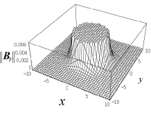
(a) t=3

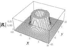
(b) t=4

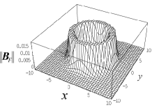
(c) t=5

Figure 1: Behavior of $||\bm{B}_{F}||$  on the plane $z=1$.

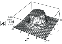
(a) t=3

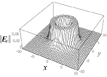
(b) t=4

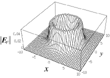
(c) t=5

Figure 2: Behavior of $||\bm{E}_{F}||$   on the plane $z=1$.

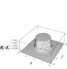
(a) t=3

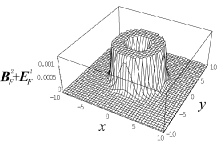
(b) t=4

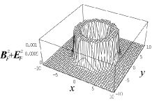
(c) t=5

Figure 3: Behavior of ${\bm{B}}_{F}^{2}+{\bm{E}}_{F}^{2}$ on the plane $z=1$.

We find that these quantities are concentrated on a circle $\sqrt{x^{2}+y^{2}}$=$f(t)$ with $f(t)$ an increasing function of $t$.
The electric current density becomes

$$\displaystyle{j_{F,x}=\frac{-4(xz-y)}{\rho^{4}(Y+1)^{2}}},\quad\displaystyle{j_{F,y}=\frac{-4(x+yz)}{\rho^{4}(Y+1)^{2}},}\quad\displaystyle{j_{F,z}=\frac{-2(1+z^{2}+t^{2}-\rho^{2})}{\rho^{4}(Y+1)^{2}}}$$ (39)

and hence

$$||\bm{j}_{F}||=\frac{2\sqrt{L^{2}-4t^{2}\rho^{2}}}{\rho^{4}(Y+1)^{2}}.$$ (40)

In Fig.4, we show the time-development of $||\bm{j}_{F}||$. We find a behavior similar to those of $||\bm{B}_{F}||$, $||\bm{E}_{F}||$ and $\bm{B}_{F}^{2}+\bm{E}_{F}^{2}$.

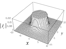
(a) t=3

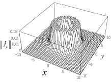
(b) t=4

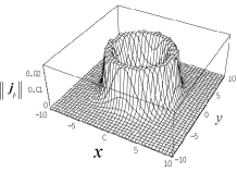
(c) t=5

Figure 4: Behavior of $||\bm{j}_{F}||$   on the plane $z=1$.

The electric charge density $\rho_{F}$ becomes

$$\displaystyle{\rho_{F}=\frac{-4tz}{\rho^{4}(Y+1)^{2}}}=\frac{-64tz}{\left[(1+t^{2}-r^{2})^{2}+4r^{2}\right]^{2}}.$$ (41)

In Fig.5, we show the time-development of $\rho_{F}$ on the plane $z=1$.

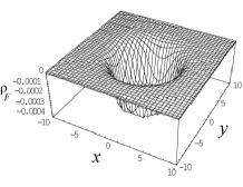
(a) t=1

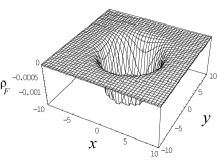
(b) t=2

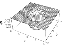
(c) t=3

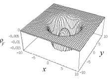
(d) t=4

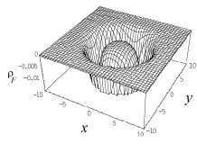
(e) t=5

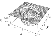
(f) t=6

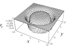
(g) t=7

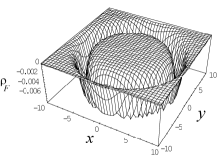
(h) t=8

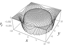
(i) t=9

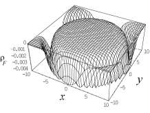
(j) t=10

Figure 5: Behavior of $\rho_{F}$   on the plane $z=1$.

On the other hand, defining $\varepsilon$ by

$$\displaystyle{\varepsilon\equiv\frac{1}{2}\int\!\!\!\int\!\!\!\int dxdydz\left(\bm{E}^{2}+\bm{B}^{2}\right)},$$ (42)

and observing

$$\displaystyle{\bm{E}^{2}=\bm{B}^{2}=\frac{64\left(1+t^{2}+r^{2}+2ty\right)^{2}}{\left[t^{4}-2t^{2}(r^{2}-1)+(r^{2}+1)^{2}\right]^{3}}},$$ (43)

we obtain

$$\varepsilon_{F}=\frac{1}{2}\varepsilon=4\pi^{2}$$ (44)

from (30), (38). This result is expected from the observation

$$\bm{B}_{F}^{2}=\bm{B}^{2}=\bm{E}^{2},\quad\bm{E}_{F}=0\quad{\rm{at}}\quad t=0.$$ (45)

At $t=0$, $\rho_{F}$ vanishes and $\bm{j}_{F}$ satisfies the relation

$$\bm{j}_{F}=\frac{8\bm{B}_{F}}{r^{2}+1}.$$ (46)

$||\bm{j}_{F}||$ simplifies to the spherically symmetric configuration $\frac{32}{(r^{2}+1)^{3}}$. The net current defined by

$$\bm{J}_{F}=\int\!\!\!\int\!\!\!\int dxdydz\bm{j}_{F}$$ (47)

is non-vanishing and is given by $\left(0,0,-\frac{8\pi^{2}}{3}\right)$.

4 Summary

We have seen that Ferreira’s solution of CNLSM defined by (1) gives rize the electromagnetic fields $\bm{E}_{F}$ and $\bm{B}_{F}$ for the charge density $\rho_{F}$ and the current density $\bm{j}_{F}$ satisfying the constraints (26). We have investigated some of their properties. We have shown that we can construct exact solutions of the CNLSM from the examples considered in the theory of electromagnetic knots. We finally note that the fields $\bm{B}_{F}$ and $\bm{E}_{F}$ are described by a simple $4$-potential [7]

$$A_{F,\mu}=\frac{1}{2}\left[(g(Y)-1)(m_{1}\partial_{\mu}\xi+m_{3}\partial_{\mu}\zeta)+m_{2}g(Y)\partial_{\mu}\varphi\right],$$ (48)

while the $4$-potential $A_{\mu}$ realising $\bm{B}_{F}$ and $\bm{E}_{F}$ is somewhat complicated [6]. The knot structure of $\bm{B}_{F}$ is inherited by the Hopf index associated with $u$. On the other hand, the knot structures of $\bm{B}$ and $\bm{E}$ are inherited by the Hopf indices associated with $\eta_{m}$ and $\eta_{e}$, respectively.

References

- [1] A.Trautman, Int. J. Theor. Phys. 16 561 (1977).
- [2] A.F.Raada, Lett. Math. Phys.18, 97 (1989).
- [3] A.F.Raada, J. Phys. A:Math. Gen. 23 L815 (1990).
- [4] A.F.Raada and J.L.Trueba, Phys. Lett. A 202 (1995).
- [5] A.F.Raada M.Solar and J.L.Trueba, Phys. Rev. E 62 7181 (2000).
- [6] W.T.M.Irvine and D.Bouwmeester, Nature Physics 4 716 (2008).
- [7] L. Ferreira, J. High En. Phys. 0603 (2006) 075. arXiv:hep-th/060123v2.
- [8] L. Faddeev, Lett. Math. Phys. 1 289 (1976).
- [9] L. Faddeev and A. J. Niemi, Nature 387 58 (1997).
- [10] O.Babelon and L. Ferreira, J. High En. Phys. 0211 (2002) 020. arXiv:hep-th/0210154v1.