Tunable pseudogap Kondo effect and quantum phase transitions in Aharonov-Bohm interferometers

Abstract

We study two quantum dots embedded in the arms of an Aharonov-Bohm ring threaded by a magnetic flux. The system can be described by an effective one-impurity Anderson model with an energy- and flux-dependent density of states. For specific values of the flux, this density of states vanishes at the Fermi energy, yielding a controlled realization of the pseudogap Kondo effect. The conductance and transmission phase shifts reflect a nontrivial interplay between wave interference and interactions, providing clear signatures of quantum phase transitions between Kondo and non-Kondo ground states.

Nanoscale quantum-dot devices are a formidable tool for probing the inherent quantum-mechanical nature of electrons. Manifestations of quantum electronic properties in these devices include wave interference in Aharonov-Bohm (AB) rings QD:interference ; Aharony:156802:2003 ; Zaffalon:226601:2008 and many-body phenomena such as the Kondo effect (the screening of a localized magnetic moment by conduction electrons) QD:Kondo ; QD:Kondo-rings ; QD:QPTs ; Zaffalon:226601:2008 and quantum phase transitions (QPTs) QD:QPTs . The interplay between quantum interference and the Kondo effect can be studied by inserting a quantum dot in an AB ring, as shown both experimentally QD:Kondo-rings and theoretically QD:Kondo-rings-theory ; Lopez:115312:2005 ; Simon:245313:2005 .

This Letter focuses on a system in which two quantum dots are embedded in the same AB ring. Interesting effects have been proposed Lopez:115312:2005 in cases where both dots are in the Kondo regime. Here, we consider instead a device in which the presence of one, effectively noninteracting dot creates for a second, Kondo-regime dot, an energy-dependent effective density of states that depends on the magnetic flux applied through the ring. Varying this flux can dramatically affect the Kondo state in the interacting dot, causing the Kondo temperature $T_{K}$—the characteristic energy scale of the Kondo state—to range over many orders of magnitude.

This two-dot AB device can also realize the conditions necessary for observation of the pseudogap Kondo effect Withoff:1835:1990 ; pseudogap-Anderson , in which coupling of a magnetic impurity to a power-law-vanishing density of conduction states gives rise to a pair of QPTs between Kondo ($T_{K}>0$) and non-Kondo ($T_{K}=0$) phases. Pseudogap Kondo physics has previously been predicted to occur in double-quantum-dot devices Dias:096603:2006 ; Dias:0804.0805:2008 , but the ring geometry of the present setup allows a deeper exploration of the interplay between coherent quantum interference and the Kondo effect. The conductance and transmission phase shift through the system exhibit clear signatures of each zero-temperature transition within a quantum-critical region that extends up to temperatures of order the maximum Kondo scale of the interacting dot. This robustness plus the relative ease of experimental control make the proposed device very promising for experimental investigation of pseudogap Kondo physics.

Model.—Quantum dots (“1” and “2”) are embedded in opposite arms of an AB interferometer that is connected to left (“$L$”) and right (“$R$”) metallic leads, as shown in Fig. 1(a). Dot 1 is in a Coulomb blockade valley and is occupied by an odd number of electrons, while dot 2 has a single noninteracting level in resonance with the leads. An external AB flux $\Phi$ passes through the interferometer, causing a phase difference $\phi=2\pi\Phi/\Phi_{0}$ ($\Phi_{0}=hc/e$) between electrons that tunnel from $L$ to $R$ via dot 1 and those that tunnel via dot 2. Provided that the flux through each quantum dot (as opposed to the entire ring) is much smaller than $\Phi_{0}$, orbital effects can be neglected. The low $g$-factor in typical GaAs devices allows one also to disregard the Zeeman splitting in the dots. In this approximation, the Hamiltonian for the setup is

$$H=\sum_{j,\sigma}\varepsilon_{j}a^{{\dagger}}_{j\sigma}a^{\phantom{{\dagger}}}_{j\sigma}+U_{1}a^{{\dagger}}_{1\uparrow}a^{\phantom{{\dagger}}}_{1\uparrow}a^{{\dagger}}_{1\downarrow}a^{\phantom{{\dagger}}}_{1\downarrow}+\sum_{\ell,\mathbf{k},\sigma}\!\varepsilon_{\ell\,\mathbf{k}}c^{{\dagger}}_{\ell\mathbf{k}\sigma}c^{\phantom{{\dagger}}}_{\ell\mathbf{k}\sigma}\\[-2.15277pt] +\sum_{j,\ell,\mathbf{k},\sigma}\bigl{(}W_{j\ell}\,a^{{\dagger}}_{j\sigma}c^{\phantom{{\dagger}}}_{\ell\mathbf{k}\sigma}+\text{H.c.}\bigr{)}\,,$$ (1)

where $a_{j\sigma}$ destroys a spin-$\sigma$ electron in dot $j$ ($j=1,2$) and $c_{\ell\,\mathbf{k}\sigma}$ destroys a spin-$\sigma$ electron of wave vector $\mathbf{k}$ and energy $\varepsilon_{\ell\,\mathbf{k}}$ in lead $\ell$ ($\ell=L,R$). Each lead is assumed to have a constant density of states $\rho(\varepsilon)=\rho_{0}\Theta(D-|\varepsilon|)$, as well as a local ($\mathbf{k}$-independent) coupling to the dots. The gauge degree of freedom allows one to write $W_{1L}=V_{1L}e^{+i\phi/4}$, $W_{1R}=V_{1R}e^{-i\phi/4}$, $W_{2L}=V_{2L}e^{-i\phi/4}$, and $W_{2R}=V_{2R}e^{+i\phi/4}$ where $V_{j\ell}$ is real. For simplicity, we consider symmetric couplings $V_{jR}=V_{jL}\equiv V_{j}/\sqrt{2}$.

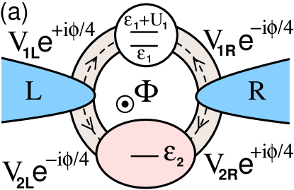
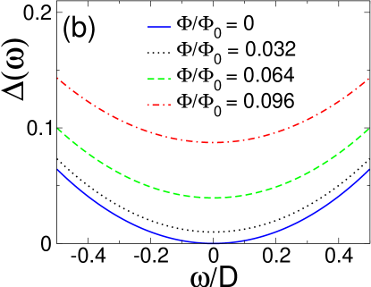
Figure 1: (Color online) (a) Schematic of the AB interferometer with embedded quantum dots, coupled to external leads ($L$ and $R$) and threaded by a magnetic flux $\Phi$. (b) Hybridization function $\Delta(\omega)$ for $\varepsilon_{2}=0$ and different values of $\Phi$.

At small bias and low temperatures, transmission through an interacting system can be described by a Landauer-like formula Meir:2512:1992 . The conductance $g$ and the transmission phase shift $\theta_{t}$ of the device are given by

$$g =\frac{2e^{2}}{h}\int d\omega\,\left(-\frac{\partial f}{\partial\omega}\right)\,|t_{LR}(\omega)|^{2}\,,$$ (2)

$$\theta_{t} =\arg\,\int d\omega\,\left(-\frac{\partial f}{\partial\omega}\right)\,t_{LR}(\omega)\,,$$ (3)

where $f(\omega,T)$ is the Fermi function at energy $\omega$ (measured from the Fermi level) and temperature $T$, and $t_{LR}(\omega)\!=\!2\pi\rho_{0}\sum_{ij}W^{*}_{iL}G_{ij}(\omega)W_{jR}$ is the transmission coefficient. Here, $G_{ij}(\omega)=-i\int_{0}^{\infty}\!dt\,e^{i\omega t}\langle\{a^{\phantom{{\dagger}}}_{i\sigma}(t),a^{{\dagger}}_{j\sigma}(0)\}\rangle$ is a standard retarded Green’s function.

The dot-1 Green’s function (calculated in the presence of dot 2 and the leads, and taking the $U_{1}$ interaction into full account) can formally be written $G_{11}(\omega)=[\omega-\varepsilon_{1}-\Sigma_{11}^{*}(\omega)-\Sigma^{(0)}_{11}(\omega)]^{-1}$, where $\Sigma_{11}^{*}$ and $\Sigma_{11}^{(0)}$ are, respectively, the interacting and noninteracting contributions to the self-energy. Standard equations of motion techniques can be used to express the remaining $G_{ij}$’s in terms of $G_{11}$ and known quantities, and to obtain the exact result

$$\Sigma^{(0)}_{11}=\sum_{\ell,\mathbf{k}}\frac{|W_{1\ell}|^{2}}{\omega\!-\!\varepsilon_{\ell\mathbf{k}}}+\!\!\!\sum_{\ell,\ell^{\prime},\mathbf{k},\mathbf{k}^{\prime}}\!\!\frac{W^{\phantom{*}}_{1\ell}W^{*}_{2\ell}}{\omega\!-\!\varepsilon_{\ell\mathbf{k}}}\frac{1}{{\omega\!-\!\varepsilon_{2}\!+\!i\Delta_{2}}}\frac{W^{\phantom{*}}_{2\ell^{\prime}}W^{*}_{1\ell^{\prime}}}{\omega\!-\!\varepsilon_{\ell^{\prime}\mathbf{k}^{\prime}}},$$ (4)

where $\Delta_{j}=\pi\rho_{0}V_{j}^{2}$. The first term in Eq. (4) describes the effect on dot 1 of coupling purely to the leads, while the second term represents an indirect coupling between the dots. In the wide-band limit $|\omega|\ll D$, these processes combine to yield an energy-dependent hybridization width $-\mbox{Im}\Sigma^{(0)}_{11}(\omega)\equiv\pi\rho_{\mathrm{eff}}(\omega)V_{1}^{2}$, with

$$\rho_{\mathrm{eff}}(\omega)=\rho_{0}\frac{(\omega-\varepsilon_{2})^{2}+\Delta_{2}^{2}\sin^{2}(\pi\Phi/\Phi_{0})}{(\omega-\varepsilon_{2})^{2}+\Delta_{2}^{2}}.$$ (5)

Then $G_{11}(\omega)$ corresponds to the Green’s function of a single Anderson impurity coupled to a density of conduction states $\rho_{\mathrm{eff}}(\omega)$ that is periodic in the applied flux. Note that $\rho_{\mathrm{eff}}(\omega)=\rho_{0}$ for $\Phi=(n+\frac{1}{2})\Phi_{0}$, where $n$ is any integer. More generally, $\rho_{\mathrm{eff}}(\omega)\simeq\rho_{0}$ for $|\omega-\varepsilon_{2}|\gg\Delta_{2}$, dipping to $\rho_{\mathrm{eff}}(\omega)\simeq\rho_{0}\sin^{2}(\pi\Phi/\Phi_{0})$ for $|\omega-\varepsilon_{2}|\ll\Delta_{2}$. For special cases where $\varepsilon_{2}=0$ and $\Phi=n\Phi_{0}$, $\rho_{\mathrm{eff}}(\omega)$ vanishes at the Fermi energy as $\omega^{2}$ [solid line in Fig. 1(b)], and the low-energy physics is that of the pseudogap Anderson model pseudogap-Anderson . In all other cases, $\rho_{\mathrm{eff}}$ is metallic and one recovers a conventional Anderson model, albeit one with a field-modulated impurity-host coupling.

This analysis raises the intriguing prospect of realizing a flux-tuned pseudogap in a two-dot AB ring device. We have solved the effective one-impurity model suggested by Eq. (5) using the numerical renormalization-group method KrishnamurthyWW80_1 ; Bulla:395:2008 to obtain properties of the full system. Below, we fix $U_{1}=0.5D$, $\Delta_{1}=0.05D$, and $\Delta_{2}=0.02D$, and show results for different values of $\varepsilon_{1}$ and $\varepsilon_{2}$ (controlled in experiments by plunger gate voltages on dots 1 and 2, respectively) and of the AB flux $\Phi$.

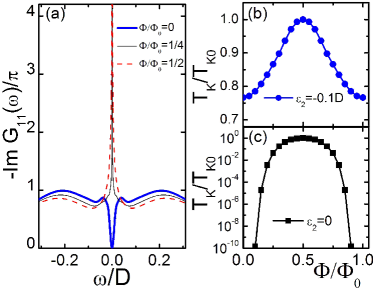
Figure 2: (Color online) (a) Dot-1 spectral function $A_{11}(\omega)$ for $\varepsilon_{1}=-U_{1}/2$, $\varepsilon_{2}=0$, and different magnetic fluxes $\Phi$. (b,c) Kondo temperature $T_{K}/T_{K0}$ vs $\Phi/\Phi_{0}$ for $\varepsilon_{1}=-\frac{1}{2}U_{1}$ and (b) $\varepsilon_{2}=-0.1D$, (c) $\varepsilon_{2}=0$. The characteristic many-body scale $T_{K0}=T_{K}(\varepsilon_{1}=-\frac{1}{2}U_{1},\Phi=\frac{1}{2}\Phi_{0})$ is independent of $\varepsilon_{2}$.

Variation of the Kondo scale.—Figure 2(a) shows the dot-1 spectral density $A_{11}(\omega)=-\pi^{-1}\mathrm{Im}G_{11}(\omega)$ for several $\Phi$ values at the special point $\varepsilon_{1}=-U_{1}/2$, $\varepsilon_{2}=0$ where the system exhibits strict particle-hole ($p$-$h$) symmetry. For a general flux, $A_{11}(\omega)$ features a Kondo resonance centered on $\omega=0$. For $\Phi=n\Phi_{0}$, however, $A_{11}(\omega)$ vanishes at $\omega=0$, signaling suppression of the Kondo effect by the pseudogap in $\rho_{\mathrm{eff}}(\omega)$ Dias:096603:2006 .

The Kondo resonance width is proportional to the Kondo temperature $T_{K}$, which we define in terms of the impurity susceptibility via the condition $T_{K}\chi_{\mathrm{imp}}(T_{K})=0.0701$ KrishnamurthyWW80_1 . $T_{K}$ values varying over three orders of magnitude under an applied magnetic field have been predicted for small AB rings containing one quantum dot Simon:245313:2005 . The present setup can greatly amplify this variation. For $|\varepsilon_{2}|\gtrsim\Delta_{2}$ [see, e.g., Fig. 2(b)], the dip in $\rho_{\mathrm{eff}}(\omega)$ around $\omega=\varepsilon_{2}$ produces only a weak field-modulation of $T_{K}$. The range of $T_{K}$ is much greater for $|\varepsilon_{2}|\lesssim\Delta_{2}$. In the extreme case $\varepsilon_{2}=0$ [Fig. 2(c)], $T_{K}$ varies from $T_{K0}$ for $\Phi=(n\!+\!\frac{1}{2})\Phi_{0}$ to zero for the pseudogap case $\Phi=n\Phi_{0}$. Here and below, $T_{K0}=T_{K}(\varepsilon_{1}\!=\!-\frac{1}{2}U_{1},\Phi\!=\!\frac{1}{2}\Phi_{0})\simeq 7\!\times\!10^{-4}D$ is a characteristic Kondo scale for dot 1 in the absence of dot 2.

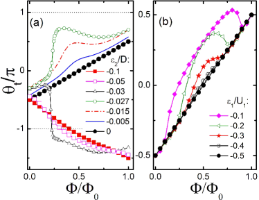
Figure 3: (Color online) Phase shift $\theta_{t}$ vs AB flux $\Phi$ at $T=0.59T_{K0}$ for (a) $\varepsilon_{1}=-U_{1}/2$ and different values of $\varepsilon_{2}$ and (b) $\varepsilon_{2}=0$ and different values of $\varepsilon_{1}$. In (a), phase lapses $\Delta\theta_{t}\simeq\pm\pi$ occur around $\varepsilon^{\mathrm{pl}}_{2}=-0.0292D$.

Quantum phase transitions.—As noted in the introduction, the presence of a pseudogap in $\rho_{\mathrm{eff}}(\omega)$ gives rise to a pair of QPTs separating Kondo and local-moment phases Dias:096603:2006 ; Dias:0804.0805:2008 . These QPTs occur in the double-dot AB setup for $\Phi=n\Phi_{0}$ and $\varepsilon_{2}=0$ when $\varepsilon_{1}$ is tuned to one of two critical values $\varepsilon_{1c}^{\pm}$. The paragraphs below describe how the system can be brought into the vicinity of one of these zero-temperature transitions by measuring the transmission phase shift $\theta_{t}(\Phi)$ and/or the conductance $g(\Phi)$ at relatively high temperatures of order $T_{K0}$.

The first step in reaching the QPT is to bring the dot-2 level $\varepsilon_{2}$ to the Fermi energy. We find that this can be most efficiently accomplished by monitoring $\theta_{t}(\Phi)$. Figure 3(a) plots $\theta_{t}$ at $T=0.59T_{K0}$ over the range $0\leq\Phi\leq\Phi_{0}$ for $\varepsilon_{1}=-U_{1}/2$ and various values of $\varepsilon_{2}$. The most striking feature is the linear variation of $\theta_{t}$ with $\Phi$ that can be used to identify the target case $\varepsilon_{2}=0$. The origin of this linearity can be seen most readily at $T=0$, where for $\varepsilon_{2}=0$, $\theta_{t}=\pi(\Phi/\Phi_{0}-\frac{1}{2})+\bar{\theta}_{t}$, with

$$\bar{\theta}_{t}=\tan^{-1}\frac{\Delta_{1}\text{Re}\,G_{11}(0)\sin^{2}(\pi\Phi/\Phi_{0})}{\Delta_{1}\text{Im}\,G_{11}(0)\sin^{2}(\pi\Phi/\Phi_{0})-1}.$$ (6)

At the pseudogap points $\Phi=n\Phi_{0}$, $\sin(\pi\Phi/\Phi_{0})=0$ and $\bar{\theta}_{t}=0$. Everywhere else, a conventional Kondo ground state forms. The special case $\varepsilon_{1}=-U_{1}/2$ and $\varepsilon_{2}=0$ shown in Fig. 3(a) exhibits an exact $p$-$h$ symmetry that ensures $\text{Re}\,G_{11}(0)=0$ and $\bar{\theta}_{t}=0$ for all $\Phi$.

Figure 3(a) also reveals interesting features away from $\varepsilon_{2}=0$. For large $|\varepsilon_{2}|$, $\theta_{t}$ evolves with increasing $\Phi$ to pass through $-\pi$ from above; since phase shifts $\theta_{t}$ and $\theta_{t}\pm 2\pi$ are equivalent, any such curve can instead be plotted with a phase jump from $-\pi$ to $\pi$, so that in all cases, $\theta_{t}(\Phi_{0})=\theta_{t}(0)+\pi$. Around $\varepsilon_{2}=\varepsilon^{\mathrm{pl}}_{2}$, “phase lapses” $\Delta\theta_{t}\simeq\pm\pi$ (not $\pm 2\pi$) appear over narrow ranges of $\Phi$ phase_lapses . For $\varepsilon_{2}>\varepsilon^{\mathrm{pl}}_{2}$, $\theta_{t}$ does not pass through $\pm\pi$, but rather varies smoothly between $\theta_{t}(0)$ and $\theta_{t}(\Phi_{0})=\theta_{t}(0)+\pi$.

For general $\varepsilon_{1}$, $\varepsilon_{2}$, and $T$, $\bar{\theta}_{t}\equiv\theta_{t}-\pi(\Phi/\Phi_{0}-\frac{1}{2})$ is small whenever $T_{K}\ll T$, and is appreciably nonzero for $T_{K}\gtrsim T$. This is illustrated in Fig. 3(b), which plots the phase shift at $T=0.59T_{K0}$ for $\varepsilon_{2}=0$ and different values of $\varepsilon_{1}$. In each case, the Kondo temperature vanishes for $\Phi=n\Phi$ and reaches its maximum value $T_{K,\max}$ at $\Phi=(n+\frac{1}{2})\Phi_{0}$. With increasing $p$-$h$ asymmetry (increasing $|\varepsilon_{1}+U_{1}/2|$), $T_{K,\max}$ decreases and the points of first noticeable deviation from linearity in $\theta_{t}$ vs $\Phi$ move closer to $\Phi=n\Phi_{0}$.

These results suggest an experimental procedure for tuning to the pseudogap: Measure $\theta_{t}$ vs $\Phi$ for different dot-2 plunger gate voltages, holding all other parameters constant, and seek to maximize the range of fluxes around $\Phi=n\Phi_{0}$ over which the phase shift satisfies $\bar{\theta}_{t}=0$. If one has truly found the dot-2 gate voltage corresponding to $\varepsilon_{2}=0$, it should in general be possible to increase the flux range over which $\bar{\theta}_{t}=0$ by stepping the plunger gate voltage on dot 1 until one achieves $\varepsilon_{1}\simeq-U_{1}/2$.

Once the dot-2 level is locked at the Fermi level, the system can be steered through (or, at any $T>0$, above) a QPT by further fine-tuning of $\varepsilon_{1}$, guided by measurements of $g(\Phi)$ and $\theta_{t}(\Phi)$. We focus on the QPT at $\varepsilon_{1}=\varepsilon_{1c}^{+}$, where $-U_{1}/2<\varepsilon_{1c}^{+}<0$, and define $\Delta\varepsilon_{1}=\varepsilon_{1}-\varepsilon_{1c}^{+}$. (A $p$-$h$ transformation maps the system from $\varepsilon_{1c}^{+}$ to the other QPT at $\varepsilon_{1c}^{-}=-U_{1}-\varepsilon_{1c}^{+}$.) As illustrated in Fig. 4, the properties at temperatures of order $T_{K0}$ reveal clear signatures of the $T=0$ transition between the local-moment ($\Delta\varepsilon_{1}<0$ and $\Phi=n\Phi_{0}$) and Kondo ($\Delta\varepsilon_{1}>0$ and/or $\Phi\neq n\Phi_{0}$) phases.

At $\Delta\varepsilon_{1}=0$ and $\Phi=n\Phi_{0}$, the finite-temperature conductance reaches a near-unitary value $g\simeq g_{0}$ [Fig. 4(a) for $n=0$] while the transmission phase shift $\theta_{t}=-\pi/2$ [Fig. 4(b)]. However, these characteristics may not be reliable experimental locators for the underlying QPT because absolute measurements of $g$ or $\theta_{t}$ may be complicated by contributions from additional (spurious) channels Aharony:156802:2003 or by the presence of stray external flux that prevents accurate identification of the point $\Phi=n\Phi_{0}$.

The derivatives of the transport properties with respect to applied flux provide a superior method for locating the transition. The critical value $\Delta\varepsilon_{1}=0$ is distinguished by two features around the pseudogap location $\Phi=n\Phi_{0}$: (i) $g$ is at a maximum [Fig. 4(a)] and (ii) $\theta_{t}$ vs $\Phi$ is linear over a significant window in $\Phi$ with a temperature-dependent slope smaller than that of the line $\bar{\theta}_{t}=0$ [Fig. 4(b)]. Figures 4(c) and 4(d) show that at three different temperatures of order $T_{K0}$, $dg/d\Phi|_{\Phi=0}$ and $d^{2}\theta_{t}/d\Phi^{2}|_{\Phi=0}$ vs $\Delta\varepsilon_{1}$ both pass through zero at $\Delta\varepsilon_{1}=0$.

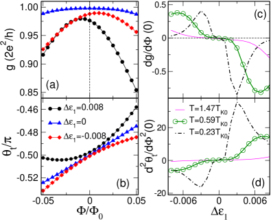
Figure 4: (Color online) Variation with $\Phi/\Phi_{0}$ of (a) the conductance $g$ and (b) the phase shift $\theta_{t}$, for $\varepsilon_{2}=0$, $T=0.59T_{K0}$, and different $\Delta\varepsilon_{1}\equiv\varepsilon_{1}-\varepsilon_{1c}^{+}$. For $\varepsilon_{2}=0$, $\Phi=0$, and different temperatures $T$, both (c) $dg/d\Phi$ and (d) $d^{2}\theta_{t}/d\Phi^{2}$ change sign at the critical value $\Delta\varepsilon_{1}=0$.

The most important conclusion to be drawn from Fig. 4 is that features indicative of the QPT are evident in the transport at least up to temperatures of order $T_{K0}$, the characteristic scale of conventional Kondo physics in the interacting dot, and one likely to be readily accessible in experiments. Figures 4(c) and 4(d) also illustrate the general property of continuous QPTs that with increasing temperature, quantum-critical behavior extends over a wider region of the parameter space. The crossings of $dg/d\Phi|_{\Phi=0}$ and $d^{2}\theta_{t}/d\Phi^{2}|_{\Phi=0}$ through zero spread over a range of $\varepsilon_{1}$ that grows roughly linearly with $T$. Similar behavior (not shown) occurs at small but nonzero $|\Phi|$ and/or $|\varepsilon_{2}|$. Away from the true critical values, however, the locations of key features (the peak in $g$ and the sign change in $d^{2}\theta_{t}/d\Phi^{2}$) depend on $T$, and below a crossover temperature these features fade away as the system enters the stable Kondo or local-moment regime.

In summary, we have studied the Kondo regime of two quantum dots embedded in the arms of an Aharonov-Bohm ring threaded by a magnetic flux. The system is described by an effective Anderson model with an effective density of states that is modulated by the external flux, allowing the Kondo temperature to be tuned over a wide range. When the ring encloses an integer multiple of the quantum of flux, the effective density of states vanishes at the Fermi energy and the setup maps onto a pseudogap Anderson model. The transmission phase shift at temperatures of order the characteristic Kondo scale of a single, interacting dot can be used to tune the device to the pseudogap regime, where the phase shift and the linear conductance exhibit clear finite-temperature signatures of underlying zero-temperature phase transitions.

We acknowledge support under NSF-DMR grants 0312939 and 0710540 (University of Florida), 0336431, 0304314 and 0710581 (Ohio University), and 0706020 (University of Tennessee/ORNL).

References

- (1) A. Yacoby, M. Heiblum, D. Mahalu, and H. Shtrikman, Phys. Rev. Lett. 74, 4047 (1995); R. Schuster et al., Nature (London) 385, 417 (1997); E. Buks et al., ibid. 391, 871 (1998); D. Sprinzak, E. Buks, M. Heiblum, and H. Shtrikman, Phys. Rev. Lett. 84, 5820 (2000); A. W. Holleitner et al., ibid. 87, 256802 (2001); K. Kobayashi, H. Aikawa, S. Katsumoto, and Y. Iye, ibid. 88, 256806 (2002); M. Sigrist et al., ibid. 93, 066802 (2004).
- (2) A. Aharony, O. Entin-Wohlman, and Y. Imry, Phys. Rev. Lett. 90, 156802 (2003).
- (3) M. Zaffalon et al., Phys. Rev. Lett. 100, 226601 (2008).
- (4) D. Goldhaber-Gordon et al., Nature (London) 391, 156 (1998); S. M. Cronenwett, T. H. Oosterkamp, and L. P. Kouwenhoven, Science 281, 540 (1998).
- (5) W. G. van der Wiel et al., Science 289, 2105 (2000); Y. Ji et al., ibid. 290, 779 (2000); Y. Ji, M. Heiblum, and H. Shtrikman, Phys. Rev. Lett. 88, 076601 (2002); U. F. Keyser et al., ibid. 90, 196601 (2003); A. Fuhrer et al., ibid. 93, 176803 (2004); R. Leturcq et al., ibid. 95, 126603 (2005).
- (6) R. M. Potok et al., Nature (London) 446, 167 (2007); N. Roch et al., ibid. 453, 633 (2008).
- (7) W. Izumida, O. Sakai, and Y. Shimizu, J. Phys. Soc. Japan 66, 717 (1997); W. Hofstetter, J. König, and H. Schoeller, Phys. Rev. Lett. 87, 156803 (2001); T. Rejec and A. Ramšak, Phys. Rev. B 68, 033306 (2003). C. H. Lewenkopf and H. A. Weidenmüller, Phys. Rev. B 71, 121309(R) (2005).
- (8) R. Lopez et al., Phys. Rev. B 71, 115312 (2005).
- (9) P. Simon, O. Entin-Wohlman, and A. Aharony, Phys. Rev. B 72, 245313 (2005).
- (10) D. Withoff and E. Fradkin, Phys. Rev. Lett. 64, 1835 (1990).
- (11) K. Ingersent, Phys. Rev. B 54, 11936 (1996); R. Bulla, T. Pruschke, and A. C. Hewson, J. Phys. Cond. Mat. 9, 10463 (1997); C. Gonzalez-Buxton and K. Ingersent, Phys. Rev. B 57, 14254 (1998); M. Vojta and R. Bulla, ibid. 65, 014511 (2001); L. Fritz and M. Vojta, ibid. 70, 214427 (2004).
- (12) L. G. G. V. Dias da Silva, N. P. Sandler, K. Ingersent, and S. E. Ulloa, Phys. Rev. Lett. 97, 096603 (2006).
- (13) L. G. G. V. Dias da Silva, K. Ingersent, N. P. Sandler, and S. E. Ulloa, Phys. Rev. B 78, 153304 (2008).
- (14) Y. Meir and N. S. Wingreen, Phys. Rev. Lett. 68, 2512 (1992).
- (15) R. Bulla, T. A. Costi, and T. Pruschke, Rev. Mod. Phys. 80, 395 (2008).
- (16) H. R. Krishna-murthy, J. W. Wilkins, and K. G. Wilson, Phys. Rev. B 21, 1003 (1980).
- (17) Phase lapses arise from a vanishing of defined by the integral in Eq. (3). With increasing , traverses the complex plane from quadrant IV to quadrant II, passing via quadrant III for , via quadrant I for , and directly through the origin for .