Optimization of mapping modes for heterodyne instruments

Abstract

Context. Astronomic line mapping with single-pixel heterodyne instruments is usually performed in an on-the-fly (OTF) or a raster-mapping mode depending on the capabilities of the telescope and the instrument. The observing efficiency can be increased by combining several source-point integrations with a common reference measurement. This is implemented at many telescopes, but a thorough investigation of the optimum calibration of the modes and the best way of performing these observations is still lacking.

Aims. We derive optimum mapping strategies and the corresponding calibration schemes based on the known instrumental performance in terms of system stability and slew times.

Methods. We use knowledge of the instrumental stability obtained by an Allan variance measurement to derive a mathematical formalism for optimizing the setup of mapping observations. Special attention has to be paid to minimizing of the impact of correlated noise introduced by the common OFF integrations and to the correction of instrumental drifts. Both aspects can be covered using a calibration scheme that interpolates between two OFF measurements and an appropriate OFF integration time.

Results. The total uncertainty of the calibrated data consisting of radiometric noise and drift noise can be minimized by adjusting the source integration time and the number of data points observed between two OFF measurements. It turns out that OTF observations are very robust. They provide a low relative noise, even if their setup deviates considerably from the optimum. Fast data readouts are often essential to minimize the drift contributions. In particular, continuum measurements may be easily spoiled by instrumental drifts. The main drawback of the described mapping modes is the limited use of the measured data at different spatial or spectroscopic resolutions obtained by additional rebinning.

1 Introduction

Mapping of astronomical objects with single pixel receivers requires a dynamical scanning of the object with the telescope, so that different coordinates are observed at different times. The observing scheme is complicated by the fact that all astronomical receivers are affected by gain instabilities (see e.g. Kraus, 1980; Rohlfs & Wilson, 1986), so that the sensitivity is a function of time as well. This dilemma can be solved by regular observations of a reference position on short time scales compared to the drift time scale. Thus all mapping schemes include a short loop for source-reference measurements and a longer timescale for scanning the whole map. One can distinguish between symmetric observing modes, where one reference measurement is done for each source point, using equal integration times in both phases, and asymmetric modes where a reference measurement is done only after observing a number of source map points. Examples of symmetric modes are dual-beam switch raster maps or frequency-switch on-the-fly maps. Each point can be treated individually and the optimum timing can be computed following the formalism developed in Ossenkopf (2008, paper I).

Asymmetric modes are position-switch on-the-fly (OTF) maps and asymmetric raster maps. In an OTF map, the telescope continuously scans the area to be mapped, while the detector integrates and data are read out at a high rate. Every individual data dump represents one point on the map, and their distance is determined by the readout rate and the scan velocity. After a finite number of points, defining one scan, the telescope slews to a position free of emission (OFF) for the reference measurement and then returns to the map for the next scan. The theoretical foundations for efficient OTF mapping schemes were laid by Mangum et al. (2000); Beuther et al. (2000), and Schieder & Kramer (2001). Asymmetric raster maps are similar to OTF maps except that dead times occur when the telescope moves between different points on a map. Because of the similarity we restrict ourselves here to analysis of OTF maps and discuss the differences for raster maps only in Appendix C. Mangum et al. (2000) has shown that OTF mapping is a very efficient mode for the observation of large fields in the sky with single-pixel receivers. The high efficiency results from the continuous scanning and integration avoiding dead times between the observation of adjacent points and from the reuse of the observation of a single reference position for the calibration of several data points. The OTF mapping imposes, however, harder requirements to the pointing and timing behavior of the telescope, which may not always be fulfilled.

Schieder & Kramer (2001) show that the knowledge of the system stability can be used to derive the optimum approach for performing actual observations. They computed the timing parameters that provide the minimum uncertainty of the calibrated data, composed of radiometric noise and drift noise, per unit observing time. Unfortunately, their computations were restricted to fluctuations with an $1/f^{\alpha}$ power spectrum with a spectral index $\alpha$ of 2 and 3. When designing the mapping observing modes for HIFI, the heterodyne instrument of the Herschel Space Observatory, to be launched in 2008 (de Graauw & Helmich, 2000), we measured, however, a wide variety of spectral drift indices (Ossenkopf, 2008). We noticed that it is important to distinguish between spectroscopic drifts, which characterize the variation of spectra after a zero-order baseline subtraction, i.e. after the correction for fluctuations that affect all channels in the same way, and total-power drifts, which characterize the variation of the raw spectra, thus being typically dominated by fluctuations of the overall gain of the instrument. Spectroscopic drifts often show values between 2 and 3, but we also noticed that many instrumental fluctuations were dominated by $1/f$ noise, i.e. following a spectral index $\alpha$ close to unity (Ossenkopf, 2008). In particular total-power drifts often show very shallow spectra. Consequently, the results from Schieder & Kramer (2001) cannot be directly applied. This requires a revision with respect to generalizing the spectral index. Moreover, Schieder & Kramer (2001) assumed a special calibration scheme for all mapping modes where single lines in a map are combined with a single reference measurement for calibration, although other calibration schemes are possible as well. We had to evaluate the profit from exploiting the possibility to scan a series of lines in alternating directions before going to the reference position. Thus we have repeated their computations in a more general framework allowing for various calibration schemes and arbitrary spectral indices resulting in general guidelines for an optimum performance and calibration of mapping observations.

Apart from the optimization of individual OTF scans discussed here, there exists a number of methods to reduce striping effects in OTF maps, in particular baseline offsets, either by an appropriate a posteriori data manipulation, assuming purely linear drifts or special correlations in the observed structures, or by a combination of multiple maps observed in different scanning directions (see e.g. Steer et al., 1984; Emerson & Gräve, 1984; Maino et al., 1999; Ashdown et al., 2007). In fact both approaches should be combined. Here we will focus on the optimum observational setup which minimizes drift effects from the very beginning, so that the measured data for all individual data points show a high quality, independent of the number of coverages in which an object is observed, so that it is also applicable to mappings of bright lines which are well detected in a single OTF map coverage. Altogether, the strategies discussed here should be

The outline of the paper follows our basic approach to the optimization problem. In Sect. 2 we introduce the properties of the OTF mapping mode and discuss the possible ways how measured data will be calibrated to obtain scientific data. In Sect. 3 we evaluate the different calibration schemes with respect to their sensitivity to drift effects. In Sect. 4 we demonstrate the application of the different calibration schemes to actual observations performed at the KOSMA 3 m telescope. From the best calibration scheme we optimize the exact timing of the observations with respect to total noise in Sect. 5. Sect. 6 discussed some limitations of OTF modes and the conclusions for the observing mode efficiencies are summarized in Sect. 7.

2 Introduction to OTF observations

2.1 The general measurement scheme

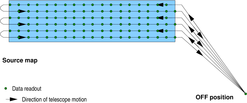
Figure 1: Sketch of an OTF observation. The dots symbolize the moments when the backends are read out. The integration starts when the telescope enters the rectangular area of the map. In this example, the OFF position is visited after every two lines and the scanning direction is alternating.

A general introduction to OTF mapping was given by Mangum et al. (2000) and Beuther et al. (2000). The general sequence of operations is demonstrated in Fig. 1. A map observation is split into individual scans and their corresponding OFF measurements. Every scan consists of $N$ source integrations obtained while continuously scanning the map. Each integration covers the time $t_{\rm s}$ spent between the edge of the map and the first readout or between two subsequent readouts, symbolized by the dots in the picture. In the example, multiple lines are combined within one scan and a turn is performed between subsequent lines so that they are scanned in opposite directions. At the end of a scan, the OFF position is visited and the reference measurement is performed with an integration time $t_{\rm OFF}$. In principle, it is possible to go from an arbitrary position within the map to the reference position. We will show later that it is preferable to complete an integer number of lines in a scan.

The measurable signal can be described by a continuous function $s(t)$. For each source point $i$ within a scan the integration provides a source count rate

$$c_{{\rm s},i}={1\over t_{\rm s}}\int_{(i-1)t_{s}}^{it_{s}}dt\;s(t)$$ (1)

if we assign $t=0$ to the start of the scan. Analogously, we can define the count rate for the OFF position as the average of the signal during the OFF integration. Because of the telescope motion during the source integration time $t_{\rm s}$, the source count rate $c_{{\rm s},i}$ corresponds to a broadened effective beam along the scanning direction. Beuther et al. (2000) have shown that for OTF maps where the readout is performed on a spatial grid corresponding to a Nyquist sampling of the map, the effective beam broadening is less than 4 %. They assumed a 14 dB edge taper corresponding to a Nyquist sampling of FPBW/2.4.

However, many observations are not performed exactly on Nyquist sampling, either by ignoring the difference between half beam width sampling and full Nyquist sampling or by using a common sampling for different tracers observed at different frequencies and consequently different beam widths. In Appx. A we show that the OTF mode does not provide a noticeable beam broadening as long as the data readout is performed on a time scale corresponding to a telescope motion of less than about 0.65 HPBW. When observations ask for a lower spatial resolution, e.g. for the comparison of line ratios, or a coarser sampling, it is possible to integrate longer, thus reducing the noise. Nevertheless, even in those cases, one should always prefer to integrate for shorter periods, if this is technically possible, to enable a further analysis of the data with the full resolution. To foresee a later manual smearing to the goal resolution, the observations then have to use a somewhat longer OFF integration time as discussed in Sect. 6, but this is usually justified by the gained flexibility.

2.2 The calibration by a reference measurement

The actual correction of the instrumental drift is done by subtracting the count rate obtained during the reference measurements at the OFF position from the count rate at the source points (Kutner & Ulich, 1981; Ossenkopf, 2002).

$$C_{{\rm s},i}=c_{{\rm s},i}-c_{\rm OFF}$$ (2)

The radiometric noise in the calibrated data for each pixel thus consists of noise contributions from the source and from the OFF integrations, $\sigma_{\rm noise}\propto\sqrt{1/t_{\rm s}+1/t_{\rm OFF}}$. In case of no dead times it can be easily shown that the radiometric noise for any total scan time $N\times t_{\rm s}+1t_{\rm OFF}$ is minimized when using an OFF integration time $t_{\rm OFF}=\sqrt{N}t_{\rm s}$, if the $N$ source integrations of one scan are calibrated with the same OFF measurement (Ball, 1976). Although this relation is not strictly fulfilled in the situation of non-negligible overheads, it remains approximately valid (Schieder & Kramer, 2001) and is thus widely used in current implementations of OTF observing modes at ground-based telescopes.

However, it is not clear that the OFF measurement at the end of an OTF scan is always the optimum reference to be used in the subtraction. Alternatively, averages of different OFF integrations may be used as reference. Therefore, we consider general case of an arbitrary reference count rate $c_{\rm R}$ with an effective integration time $t_{\rm R}$. We can distinguish three main calibration approaches:
i) single OFF: The reference position is observed for $t_{\rm R}=t_{\rm OFF}$ before (or after) a series of $N$ source points and the OFF count rate is subtracted from all source points in the scan:

$$C_{{\rm s},i}=c_{{\rm s},i}-c_{\rm R}$$ (3)

where the index $i$ running from 1 to $N$ characterizes the different source points in a series. This approach is currently used as standard calibration for OTF observations at the JCMT, MOPRA and KOSMA telescopes.

ii) interpolated OFF: The total OFF integration time $t_{\rm OFF}$ is split into two OFF observations with half the integration time, $t_{\rm R}=t_{\rm OFF}/2$, before and after the series of $N$ source points. The reference count rate subtracted from each source count rate is given by the linear interpolation between the two OFF measurements

$$C_{{\rm s},i}=c_{{\rm s},i}-[(1-l)c_{\rm R,1}+lc_{\rm R,2}]\;,$$ (4)

i.e. we use a new reference that is constructed from two OFF measurements with the half duration. Here, $l$ is a time interpolation factor being $l=0$ if the source count rate is measured at the time of the first OFF observation and $l=1$ if it is measured at the time of the second OFF. It can be obtained from

$$l={{t_{\rm R}/2+t_{\rm d,1}+(i-1/2)t_{\rm s}}\over{t_{\rm R}+t_{\rm d,1}+t_{\rm d,2}+Nt_{\rm s}}}={{t_{\rm R}/2+t_{\rm d,1}+(i-1/2)t_{\rm s}}\over{t_{\rm R}+t_{\rm scan}}}$$ (5)

where the terms $t_{\rm d,1}$ and $t_{\rm d,2}$ stand for the dead times due to the telescope from the OFF position to the first source point and from the last source point to the OFF position. The number $i$ denotes the index of the source point in the current scan and $t_{\rm scan}=t_{\rm d,1}+Nt_{\rm s}+t_{\rm d,2}$ denotes the total duration of a scan.

The actual timing of the observation can be almost identical to case i because the OFF measurements between the scans are simply split into two subsequent OFF measurements with half duration. The only difference is that the whole observation is bracketed between two OFF measurements with $t_{\rm R}=t_{\rm OFF}/2$. This approach is currently the default setting for the OTF calibration at the IRAM 30 m telescope.

iii) double OFF: This approach uses the same splitting of the OFF measurement into two parts before and after the source series as case ii but uses the average of both count rates for the calibration instead of applying a linear interpolation in time:

$$C_{{\rm s},i}=c_{{\rm s},i}-\left[{1\over 2}c_{\rm R,1}+{1\over 2}c_{\rm R,2}\right]\;.$$ (6)

It corresponds to Eq. (4) with a fixed value $l=0.5$. In this approach all source points in a scan are calibrated with the fixed OFF count rate corresponding to the value at the center of the scan in the linear interpolation. This calibration scheme is available as optional mode at several ground-based telescopes.

For all following computations we will stick to Eq. (4), which can be used for all calibration schemes when applying the appropriate weighting factors $l$ and $1-l$. For the case of the single OFF $l$ is set to 1 or 0, for the interpolated OFF Eq. (5) is used, and for the double OFF $l=1/2$.

The obvious advantage of the linear interpolation (ii) is the complete cancellation of linear drifts. The disadvantage is the production of a varying noise across each series of source points resulting from the variable OFF contributions. In the center of each series, where $l=0.5$, the noise from the OFF position corresponds to an integration time of $t_{\rm OFF}$, but at the ends, where $l=0$ or $l=1$, the noise from the OFF is higher by $\sqrt{2}$ because only a single measurement with $t_{\rm R}=t_{\rm OFF}/2$ contributes. This is actually visible in some IRAM observations where the noise is minimal in the center of each line but increasing towards the edges of the maps (Teyssier, priv.comm.). The effect is relatively small for long scans with $t_{\rm OFF}=\sqrt{N}t_{\rm s}$ because the contribution from the OFF integration to the total noise is small. Its change by a factor $\sqrt{2}$ is hardly noticeable in most cases.

2.3 Correlated noise

The calibration of data from several source points with a common OFF measurement always produces some artificial correlation in the final maps because the noise from the OFF measurement shows up in multiple points. When smoothing such a map to lower resolution the noise does not decrease with the square root of the number of points averaged, but the noise contribution from the OFF will remain constant. We can describe this as “correlated noise given by the noise variance contribution from the OFF measurement and the number of map points affected by this contribution. From Eq. (4) we can see that the noise variance contribution from the OFF measurement to an individual source point follows

$$\sigma_{\rm R}^{2}\propto{(1-l)^{2}\over t_{\rm R,1}}+{l^{2}\over t_{\rm R,2}}$$ (7)

assuming statistically independent noise in the OFF measurements involved.

The different ways of adding the noise from the neighboring OFF measurements in the different calibration approaches result in a different amount of correlated noise throughout an OTF map. For the single-OFF calibration, with $l=0$ or $1$ and $t_{\rm R}=t_{\rm OFF}$ we find a constant contribution from one reference measurement to all points of a scan.

When splitting the OFF measurement between the OTF scans into two parts with half the integration time, $t_{\rm R}=t_{\rm OFF}/2$, the noise variance in each of these parts is twice the noise of the original measurement. For the double-OFF calibration with a fixed ratio $l=1/2$ each source point inherits a quarter of the noise variance from each of the OFF measurements. Consequently their individual contribution falls at half of the level from the single-OFF calibration. The sum of their contributions provides a noise level identical to the single-OFF treatment.

When the calibration involves a temporal change as for the linearly interpolated-OFF calibration, the OFF noise will also vary from point to point. The linear interpolation between the two OFF measurements bracketing a scan with $t_{\rm R}=t_{\rm OFF}/2$ creates an OFF noise contribution that increases quadratically towards the boundaries of the scans. Compared to the single-OFF calibration the noise sum is higher by the factor $1+4(l-1/2)^{2}$. The noise variance changes within a factor two matching the value for the single-OFF calibration at the scan center, but being two times as high at the boundaries.

We can quantify the impact of this OFF noise as correlated noise within the map by the simple parameter $\sigma_{\rm combined}^{2}$, given by the product of the number of pixels showing the same noise contribution and the variance of this noise. This definition reflects the visual effect of correlated noise in a map where the eye automatically tends to integrate over parts of the map to detect structures. The product of variance and pixel number corresponds to this integration. For all calibration schemes discussed so far, the correlated noise is restricted to single scans and can be approximated by integrating the individual noise contributions in Eq. (7) over the scan length ignoring the discretization of the scan in terms of source points.

The single-OFF calibration and the double-OFF calibration produce the same correlated noise sum, as each point of a scan is treated with the same OFF noise variance in both cases. For the interpolated-OFF calibration, however, we find a correlated noise sum, $\sigma_{\rm combined}^{2}$, which amounts to only 2/3 of the value in the single-OFF calibration, because the contributions from the individual noise measurements vary quadratically across a scan (Eq. 7). Although the average total noise sum amounts to 4/3 of the value from the single-OFF calibration we have a lower correlated noise. The linear interpolation thus shows a slightly increased total noise but a decreased correlated noise contribution compared to the single-OFF scheme.

An obvious further step towards an increase of the efficiency of the observations is the reuse of an OFF measurement for two two adjacent scans so that the OFF integration time can be reduced by a factor two. When using the full OFF integration time for the reference time, i.e. $t_{\rm R}=t_{\rm OFF}$, all the equations from Sect. 2.2 are still valid. The total noise variance is not changed, but we create additional correlations between the noise in different pixels. The correlated noise sum is increased by a factor two, because the noise from one OFF measurement is spread across the two adjacent scans. For the interpolated-OFF calibration with a reuse of the OFF data for both adjacent scans the correlated noise sum and the average total noise variances are larger by a factor 4/3 relative to the value obtained in the single-OFF calibration. Vice versa we can use an OFF calibration time of 2/3 of the time used in the single-OFF calibration to obtain the same amount of total noise and correlated noise in the interpolated-OFF calibration.

With respect to the radiometric noise we have thus the situation that single-OFF and double-OFF calibration produce the same total noise contribution and the same correlated noise contribution from the OFF measurement to each source measurement.For the double-OFF integration we could reduce the OFF integration time by a factor two still maintaining the same total noise contribution, but at cost of a higher correlated noise. In the interpolated-OFF calibration we need only an OFF integration time of 2/3 compared to the single-OFF calibration to obtain the same noise values, but on top of that we achieve a complete cancellation of all linear drift errors.

After these general considerations we will actually compute the error in the calibrated data due to both instrumental drift and the radiometric noise both from the source points and from the OFF subtraction in the next section.

3 The data uncertainty due to noise and drift

3.1 Quantitative estimate

The total uncertainty of the measured data is given by the sum of the uncertainties from radiometric noise and instrumental drifts. With known fluctuation spectra $S(f)\propto 1/f^{\alpha}$ for the two contributions the total data uncertainty can be computed as demonstrated by Schieder & Kramer (2001). They performed the estimate for the special case of a single-OFF calibration and spectral indices of the instrumental fluctuations $\alpha=2,3$. Here, we repeat these computations for the general case.

If we write the expression for the calibrated data (Eq. 2) for an arbitrary start time $t$ and the general calibration approach expressed by the weighting factor $l$ we obtain

$$C_{{\rm s},i} = c_{{\rm s},i}(t)-(1-l)c_{\rm R,1}(t)-lc_{\rm R,2}(t)$$ (9)

$$= {1\over t_{\rm s}}\int_{t+t_{\rm R}+t_{\rm D,1}}^{t+t_{\rm R}+t_{\rm D,1}+t_{\rm s}}dt^{\prime}\;s(t^{\prime})$$

$$-(1-l){1\over t_{\rm R}}\int_{t}^{t+t_{\rm R}}dt^{\prime}\;s(t^{\prime})-l{1\over t_{\rm R}}\int_{t+t_{\rm scan}+t_{\rm R}}^{t+t_{\rm scan}+2t_{\rm R}}dt^{\prime}\;s(t^{\prime})\;.$$

To abbreviate the notation we use here the total delay time before a given source measurement $i$, $t_{\rm D,1}=t_{\rm d,1}+(i-1)t_{\rm s}$. In the same way we define $t_{\rm D,2}$ as the total delay time after a given source measurement $i$, $t_{\rm D,2}=t_{\rm scan}-t_{\rm D,1}-t_{\rm s}=t_{\rm d,2}+(N-i)t_{\rm s}$. With the appropriate weighting factors $l$ and $1-l$, the equation can be used for all calibration schemes discussed above. In all schemes where the OFF measurement is split into two separate contributions we use $t_{\rm R}=t_{\rm OFF}/2$, otherwise $t_{\rm R}=t_{\rm OFF}$.

Assuming ergodicity we can obtain the average total uncertainty of the count rate from a time-average

$$\sigma_{C}^{2}(i)=\left\langle(C_{{\rm s},i}-\langle C_{{\rm s},i}\rangle_{t})^{2}\right\rangle_{t}$$ (10)

where we treat the measurement as a continuous function, ignoring that it is performed only in discrete steps.

It can be easily seen that the maximum uncertainty occurs for weak signals where the count rates on the source and on the OFF position basically are the same. Thus we consider the worst case assuming $\langle c_{{\rm s},i}(t)-(1-l)c_{\rm R,1}(t)-lc_{\rm R,2}(t)\rangle_{t}=0$. Then the second term in Eq. (10) vanishes and we can rewrite it as

$$\sigma_{C}^{2}(i) = \left\langle c_{{\rm s},i}(t)^{2}\right\rangle_{t}+(1-l)^{2}\left\langle c_{\rm R,1}(t)^{2}\right\rangle_{t}+l^{2}\left\langle c_{\rm R,2}(t)^{2}\right\rangle_{t}$$ (11)

$$-2(1-l)\left\langle c_{{\rm s},i}(t)c_{\rm R,1}(t)\right\rangle_{t}-2l\left\langle c_{{\rm s},i}(t)c_{\rm R,2}(t)\right\rangle_{t}$$

$$+2l(1-l)\left\langle c_{\rm R,1}(t)c_{\rm R,2}(t)\right\rangle_{t}\;.$$

The first three contributions contain the variation representing the noise within each of the three measurements involved. The other terms represent the cross correlation between them containing the mutual drift terms.

The computation of all six terms follows the same approach. We demonstrate it here only for $\left\langle c_{{\rm s},i}(t)c_{\rm R,1}(t)\right\rangle_{t}$:

$$\left\langle c_{{\rm s},i}(t)c_{\rm R,1}(t)\right\rangle_{t}={1\over t_{\rm s}t_{\rm R}}\left\langle\int_{t}^{t+t_{\rm R}}dt^{\prime}\int_{t+t_{\rm R}+t_{\rm D,1}}^{t+t_{\rm R}+t_{\rm D,1}+t_{\rm s}}dt^{\prime\prime}\;s(t^{\prime})s(t^{\prime\prime})\right\rangle_{t}\;.$$ (12)

With the coordinate transformation to time variables $\tau^{\prime}=t+t_{\rm R}-t^{\prime}$ and $\tau^{\prime\prime}=t+t_{\rm R}-t^{\prime\prime}$ we obtain

$$\left\langle c_{{\rm s},i}(t)c_{\rm R,1}(t)\right\rangle_{t}\! =\! {1\over t_{\rm s}t_{\rm R}}$$

$$\times\! \int_{0}^{t_{\rm R}}d\tau^{\prime}\int_{0}^{t_{\rm s}}d\tau^{\prime\prime}\left\langle s(t-\tau^{\prime})s(t-\tau^{\prime\prime}+t_{\rm D,1}+t_{\rm s})\right\rangle_{t}$$

where we have also exchanged the sequence of integration and time-averaging. The integrals can be evaluated using the auto-correlation function of the fluctuation spectrum. For a power-law noise spectrum $S(f)\propto 1/f^{\alpha}$ with spectral indices $0<\alpha\leq 3$ the auto-correlation function can be evaluated as

$$\gamma(\tau) = \langle s(t+\tau)s(t)\rangle_{t}$$ (14)

$$= g_{0}-g_{\alpha}|\tau|^{\alpha-1}$$

assuming zero averages (Schieder & Kramer, 2001). This relation and the properties of this kind of autocorrelation functions are extensively used in studies of fractal and turbulent processes (e.g. Peitgen & Saupe, 1988; Bunde & Havlin, 1994; Frisch, 1995).

Exploiting this relation, the integration can be carried out as demonstrated in Appendix B resulting in

$$\left\langle c_{{\rm s},i}(t)c_{\rm R,1}(t)\right\rangle_{t} = g_{0}-{g_{\alpha}\over\alpha(\alpha+1)t_{\rm s}t_{\rm R}}\left\{[t_{\rm D,1}+t_{\rm s}+t_{\rm R}]^{\alpha+1}\right.$$

$$\qquad\left.-[t_{\rm D,1}+t_{\rm R}]^{\alpha+1}-[t_{\rm D,1}+t_{\rm s}]^{\alpha+1}+t_{\rm D,1}^{\alpha+1}\right\}$$

We can perform the integration for all terms in Eq. (11) and obtain

$$\sigma_{C,\alpha}^{2}(i)={-2g_{\alpha}\over\alpha(\alpha+1)}\bigg{\{}t_{\rm s}^{\alpha-1}+(1-2l+2l^{2})t_{\rm R}^{\alpha-1}$$

$$+l(1-l){(2t_{\rm R}+t_{\rm scan})^{\alpha+1}-2(t_{\rm R}+t_{\rm scan})^{\alpha+1}+t_{\rm scan}^{\alpha+1}\over t_{\rm R}^{2}}$$

$$-(1-l){(t_{\rm R}+t_{\rm D,1}+t_{\rm s})^{\alpha+1}\!-\!(t_{\rm R}+t_{\rm D,1})^{\alpha+1}\!-\!(t_{\rm D,1}+t_{\rm s})^{\alpha+1}\!+\!t_{\rm D,1}^{\alpha+1}\over t_{\rm R}t_{\rm s}}$$

$$\left.-l{(t_{\rm R}+t_{\rm D,2}+t_{\rm s})^{\alpha+1}-(t_{\rm R}+t_{\rm D,2})^{\alpha+1}-(t_{\rm D,2}+t_{\rm s})^{\alpha+1}+t_{\rm D,2}^{\alpha+1}\over t_{\rm R}t_{\rm s}}\right\}\;.$$

The first two terms contain the fluctuations within the source and the OFF measurements (Eq. 26), the third term represents the drift between the two involved OFF measurements and the last two terms characterize the drift between the source measurement and the two OFF measurements.

The coefficient $g_{\alpha}$ giving the amplitude of the fluctuations can be determined by an Allan variance measurement (Allan, 1966). The Allan variance measures the variance of the difference of the signal between subsequent intervals in a long time series of data dumps as a function of the length of the intervals. A comprehensive introduction to this technique was given in paper I. The Allan variance spectrum can be computed in the same way as laid out above assuming zero delays For $l=0$, $t_{\rm s}=t_{\rm R}=t_{\rm bin}$, and $t_{\rm D,2}=t_{\rm D,2}=0$ we can transform Eq. (3.1) into

$$\sigma_{\rm A,\alpha}^{2}={2g_{\alpha}\over\alpha(\alpha+1)}\;4(2^{\alpha-1}-1)t_{\rm bin}^{\alpha-1}$$ (17)

where $t_{\rm bin}$ denotes the length of the data intervals. This allows us to express the uncertainty of the calibrated OTF data in terms of the Allan variance spectrum.

However, the fluctuations of any signal are not only characterized by a single power spectrum but they consist at least of a superposition of white noise with a spectral index $\alpha=0$ and an instrumental drift contribution with some steeper spectral index $\alpha$. Fortunately, we expect no correlation between the radiometric white noise and the instrumental drift, so that both the Allan variance spectrum and the uncertainty of the calibrated data from an OTF observation simply are the sum of both contributions, $\sigma_{\rm A}^{2}=\sigma_{\rm A,0}^{2}+\sigma_{\rm A,\alpha}^{2}$ and $\sigma_{\rm C}^{2}=\sigma_{\rm C,0}^{2}+\sigma_{\rm C,\alpha}^{2}$. The Allan variance of the white noise contribution is given by

$$\sigma_{\rm A,0}^{2}={2\langle s(t)\rangle_{t}^{2}\over B_{\rm Fl}t_{\rm bin}}$$ (18)

and the white noise contribution to the OTF measurement is

$$\sigma_{\rm C,0}^{2}={\langle s(t)\rangle_{t}^{2}\over B_{\rm Fl}}\left({1\over t_{\rm s}}+{1-2l+2l^{2})\over t_{\rm R}}\right)$$ (19)

where $B_{\rm Fl}$ denotes the fluctuation bandwidth of the radiometric noise.

With the definition of the Allan time $t_{\rm A}$ as the bin size $t_{\rm bin}$ where the drift contribution and the radiometric noise in the measured Allan variance spectrum show the same magnitude (paper I), we can relate the radiometric noise to the coefficient $g_{\alpha}$. We obtain the coefficient of the drift contribution as

$$g_{\alpha}={\alpha(\alpha+1)\langle s(t)\rangle_{t}^{2}\over 4(2^{\alpha-1}-1)B_{\rm Fl}t_{\rm A}^{\alpha}}\;.$$ (20)

Finally we can compare the total uncertainty of the calibrated data $\sigma_{C}^{2}(i)$ to the unavoidable uncertainty due to the radiometric noise in an equivalent measurement with an ideal instrument without any drifts, in an ideal observation without the need for an OFF measurement. If we assume that this observation uses the total observing time for the $N$ points of an OTF cycle in a given map, $t_{\rm tot}=t_{\rm OFF}+t_{\rm scan}$, the resulting data uncertainty is

$$\sigma_{C,{\rm ideal}}^{2}={N\langle s(t)\rangle_{t}^{2}\over B_{\rm Fl}t_{\rm tot}}\;.$$ (21)

When we combine Eqs. (20) and (21) to substitute $g_{\alpha}$, add the radiometric and drift noise contributions $\sigma_{\rm C,0}^{2}$ and $\sigma_{\rm C,\alpha}^{2}$ and normalize the resulting noise of the real OTF observation relative to the limiting ideal observation we obtain a measure for the actual impact of all instrumental effects on the data quality

$${\sigma_{C}^{2}(i)\over\sigma_{C,{\rm ideal}}^{2}}={x_{\rm tot}\over N}\left\{{1\over x_{\rm s}}+{1-2l+2l^{2}\over x_{\rm R}}\right.$$

$$-{2\over 4(2^{\alpha-1}-1)}\bigg{[}x_{\rm s}^{\alpha-1}+(1-2l+2l^{2})x_{\rm R}^{\alpha-1}$$

$$+l(1-l){(2x_{\rm R}\!+\!x_{\rm scan})^{\alpha+1}\!-\!2(x_{\rm R}\!+\!x_{\rm scan})^{\alpha+1}\!+\!x_{\rm scan}^{\alpha+1}\over x_{\rm R}^{2}}$$

$$-(1-l){(x_{\rm R}\!+\!x_{\rm D,1}\!+\!x_{\rm s})^{\alpha+1}\!-\!(x_{\rm R}\!+\!x_{\rm D,1})^{\alpha+1}\!-\!(x_{\rm D,1}\!+\!x_{\rm s})^{\alpha+1}\!+\!x_{\rm D,1}^{\alpha+1}\over x_{\rm R}x_{\rm s}}$$

$$\left.\left.-l{(x_{\rm R}\!+\!x_{\rm D,2}\!+\!x_{\rm s})^{\alpha+1}\!-\!(x_{\rm R}\!\!+\!x_{\rm D,2})^{\alpha+1}\!-\!(x_{\rm D,2}\!+\!x_{\rm s})^{\alpha+1}\!+\!x_{\rm D,2}^{\alpha+1}\over x_{\rm R}x_{\rm s}}\right]\right\}$$

where we have transformed all time scales relative to the Allan time $t_{\rm A}$ with $x_{\rm tot}=t_{\rm tot}/t_{\rm A}$, $x_{\rm s}=t_{\rm s}/t_{\rm A}$ and so on.

We find two essential contributions: the first two terms characterize the radiometric noise of the observations. This noise is higher than the radiometric noise in the ideal observation due to the $x_{\rm R}$-term containing the noise from the OFF measurement. Without this term the radiometric noise ratio would be unity. All terms in the brackets characterize the drift contribution to the total data uncertainty. The different terms stand here for the drift occurring during the different time lags involved in the measurement. The ratio between the drift noise and the radiometric noise of the observed data can be computed by simply dividing these two contributions.

3.2 Comparison of the different calibration schemes

With Eq. (3.1) we can draw quantitative conclusions on the different calibration schemes. We have computed the data uncertainty $\sigma_{C}^{2}(i)/\sigma_{C,{\rm ideal}}^{2}$ as a function of the scan length $N$, the spectral index of the instrumental drift $\alpha$, the position of a source point within the OTF scan i, the source point integration time $x_{\rm s}$, and the dead times between the OFF measurement and the source integrations in the scan. To avoid too many parameters in the following examples we simplify them by assuming that the two dead times for moving from the source to the OFF position and vice versa are the same, $x_{\rm d,1}=x_{\rm d,2}$. This is well fulfilled for most observations with the Herschel satellite and still a reasonable approximation for most ground-based telescopes. Moreover, we assume in this section that the total integration time on the OFF position follows the standard rule $x_{\rm OFF}=\sqrt{N}x_{\rm s}$ derived for an ideal telescope.

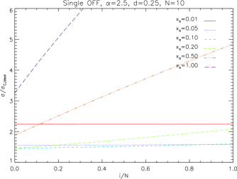
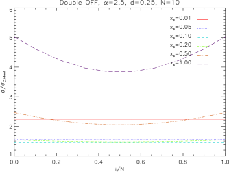
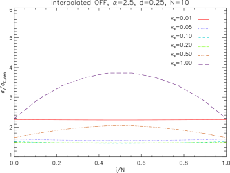
Figure 2: Variation of the total data uncertainty across an OTF scan obtained in the different OTF calibration schemes. The RMS of the fluctuations is plotted relative to the RMS which would be obtained by an ideal instrument in the same total time. Part a shows the result from the single-OFF calibration with the OFF measured before the scan, b the double-OFF calibration, and c the interpolated-OFF calibration. A scan length $N=10$, a spectral index $\alpha=2.5$, and a total dead time $x_{\rm d,1}+x_{\rm d,2}=0.25$ were used.

In Fig. 2 we compare the three standard calibration schemes from Sect. 2.2 for an example scan consisting of $N=10$ points. In the simulation a spectral index of the instrumental drift $\alpha=2.5$ was used, typical of spectroscopic fluctuations (Schieder & Kramer, 2001; Ossenkopf, 2008), and the total dead time given as the sum of the dead times before and after an OFF measurement was assumed to be a quarter of the Allan time which is a typical value for many Herschel observations. The figure shows the normalized total noise RMS as a function of the position of a source point within the scan for different source integration times $x_{\rm s}$.

For all three cases we find that the shortest integration time, $x_{\rm s}=0.01$, results in a relatively high noise. This can be easily understood by the low efficiency of this observation where only a short integration time is spent on the source but a large fraction of the total cycle is occupied by the dead times. In this relatively fast cycle no instrumental drifts are seen and the noise is barely varying across the scan. The variation of the radiometric noise across the scan by up to 11 % for a 10-points scan in the interpolated-OFF calibration scheme discussed in Sect. 2.2 actually is much lower because all 10 points are measured close to the center of the time interval between the two OFF measurements.

In contrast, we find a strong noise variation across the scan for all calibration schemes when the source integration time per point is in the order of the Allan time. All data are dominated by instrumental drifts also leading to a high total noise. An intermediate integration time per source point results in the lowest overall data uncertainty. In this example the optimum falls between about 0.1 Allan times for the single-OFF calibration and 0.2 Allan times for the interpolated-OFF calibration. Further parameter studies show that the optimum falls at shorter integration times for shorter dead times and for larger numbers of source points in a scan.

Comparing the calibration schemes shows extreme differences in the impact of the instrumental drift. The single-OFF calibration has a huge sensitivity to instrumental drifts. When using the OFF measurement before the scan for calibration, as shown in the figure, the total data uncertainty grows monotonically towards the end of the scan, for $x_{s}=1$ it exceeds even the selected plot range going up to a value of 11. For the corresponding scheme using the OFF after the scan, the plot would be mirrored. The advantage of the interpolated-OFF calibration relative to the double-OFF calibration is also clearly visible. The latter has a much larger data uncertainty at the ends of the scan due to instrumental drifts. Compared to this uncertainty, the variation of the radiometric noise from the OFF calibration in the interpolated-OFF scheme, well noticeable only for $x_{\rm s}=0.05$, is a very small contribution. In the center of the scan double-OFF and interpolated-OFF calibration necessarily have to agree. For all cases with a noticeable instrumental drift, the interpolated-OFF calibration is superior to the double-OFF calibration. The latter one is slightly better for fast scans where instrumental drifts play no role.

When performing the same computations for longer OTF scans, which are usually used when mapping large areas on the sky with ground-based telescopes, we find the same qualitative behavior as shown in Fig. 2, but an increase of all drift effects, due to the longer times covered, and a further reduction of the radiometric noise variation across the scan, so that this turns invisible in the corresponding plots. An extended parameter study has shown that the data uncertainty due to drift effects grows with the spectral index of the fluctuation spectrum $\alpha$ and with the dead times before and after the OFF measurements. For $1/f$ spectra, we obtain a very weak dependence of the maximum drift noise on the integration time, the scan length or the dead time. For moderate scan lengths, $\la 100$ points, and integration times covering a noticeable fraction of the Allan time, the maximum total noise RMS is always approximately twice the ideal noise RMS. However, $1/f$ spectra are often also correlated with very short Allan times, then limiting the observations. One has to be aware that all time scales have to be considered relative to the Allan time. For steeper noise spectra, the drift provides the main limitation to the possible scan lengths. Dead time, Allan time and drift index are determined by instrument and telescope so that their design should be directed towards a minimization. The main prerequisite for any accurate mapping observation is a a low instrumental drift expressed by a long Allan time and/or a shallow drift index.

One can still improve the observing efficiency by an appropriate calibration scheme and an optimized setup of the observations. The drift uncertainty is increased by a larger number of source points in each scan but reduced in the case of shorter integration times per source point. The mutual optimization of these two parameters leads in general to the smallest uncertainties for scans with a large number of points but very short integration times. This may be limited, of course, by the size of the region to be mapped and data rate which can be taken with the instrument. A detailed optimization taking both effects into account is given in Sect. 5.1.

Looking at the overall pictures it is clear that the interpolated-OFF approach is in general the most robust one. The single-OFF calibration is easily disqualified compared to the other two schemes. The double-OFF calibration can be slightly better than the interpolated-OFF calibration if the integration time is very short and we have an accurate knowledge of the instrumental drift behavior. Taking the usual uncertainty and the statistical fluctuations of the actual drift behavior into account, leads us, however, to the general preference of the interpolation scheme. These results hold independent of the possible split or combination of the OFF integrations with respect to the neighboring scans (Sect. 2.3) as this would only affect the correlated noise sum, not changing the noise amplitude computed here.

4 Application to observed data

The different calibration schemes were tested using existing molecular line observations performed with the KOSMA 3 m telescope. An arbitrary OTF patch was taken from a larger survey ¹³CO 2-1 survey of the Cygnus X region (Schneider et al., 2006). The observations were taken in the ordinary OTF mode where after each line of the patch, containing 20 source integrations of 5 s, one OFF integration of 23 s, corresponding to $\sqrt{20}\times 5$ s, was performed. For the slew from the end of an OTF scan to the OFF position a dead time of 19 s was needed, the slew from the OFF position to the beginning of the subsequent OTF scan took 12 s. The spectral resolution of the used backend is 360 kHz and the corresponding fluctuation bandwidth 560 kHz. The spectroscopic Allan time of the instrument at this resolution is about 120 s. The Allan time of the whole system including the atmosphere is estimated to be approximately 80 s. The drift index of the fluctuations falls between 2 and 3. For all computations we assume 2.5 here. The single-sideband system temperature during the observations was about 350 K.

To emphasize the drift effects we first consider maps of line integrated intensities, where the full velocity range of the ¹³CO line from 4 to 8 km/s was integrated corresponding to an effective bin width of 2.9 MHz. As the binning reduces the radiometric noise of the data, this corresponds to a reduction of the Allan time, where radiometric and drift noise have equal amplitudes. Following the formalism developed in Ossenkopf (2008) we can compute an effective Allan time at 2.9 MHz bin width of about 30 s. One OTF cycle corresponds to approximately five Allan times at this resolution so that we expect to notice drift effects in the integrated maps.

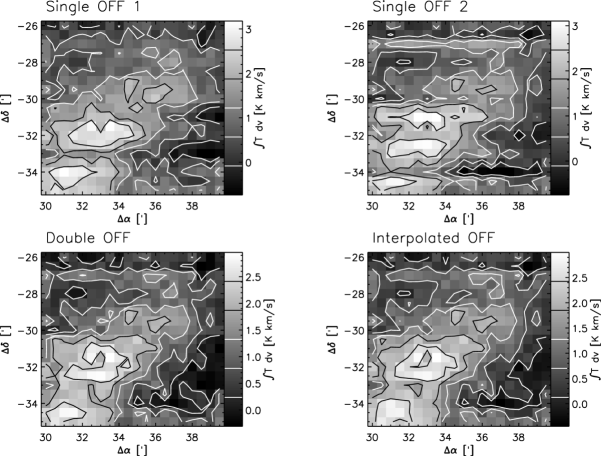
Figure 3: Demonstration of the influence of the different calibration schemes on the appearance of the produced line maps. The maps in the upper panels were obtained when calibrating with the single OFF measurement before and after each line. The lower left panel shows the result with a fixed sum from the two adjacent OFF measurements ($l=1/2$) and the lower right panel shows the result when using a time interpolation between both OFF measurements. The map was measured in horizontal stripes. After each line an OFF measurement was taken.

Figure 3 shows the integrated line maps obtained in the different calibration schemes. We can compare the observed structure with the noise computed from Eq. (3.1). An ideal observation, spending all the observing time for the map integration, would result in a radiometric noise of $\sigma\approx 0.1$ K (see Eq. 21). Due to overheads and the noise contribution from the OFF measurement, the actual radiometric noise is higher by a factor between 1.31, obtained for the double-OFF calibration and in the scan center for the interpolated-OFF calibration, and 1.37 for the single-OFF calibration. The drift noise $\sigma_{C,{\rm drift}}$ varies across the 20 points of the scan between 0.65 and 0.72 $\sigma_{C,{\rm rad.}}$ for the double-OFF calibration, between 0.56 and 0.65 $\sigma_{C,{\rm rad.}}$ for the interpolated-OFF calibration, between 0.77 and 1.45 $\sigma_{C,{\rm rad.}}$ for the single-OFF calibration using the OFF before the scan, and between 0.82 and 1.49 $\sigma_{C,{\rm rad.}}$ for the single-OFF calibration using the OFF after the scan. While the drift noise should be hidden in the radiometric noise for the double-OFF and the interpolated-OFF calibrated data, it should be clearly noticeable in the single-OFF calibrated maps towards the ends of the scans which are most apart from the corresponding OFF measurement.

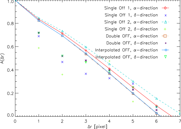
Figure 4: Autocorrelation function for the maps from Fig. 3 measured in the two perpendicular directions $\alpha$ and $\delta$. To emphasize the scan direction $\alpha$, the symbols for that direction are connected by lines. For an isotropic structure both directions should show the same values.

We can clearly recognize the very “stripy” structure in the two single-OFF calibration maps, but the stripes are not restricted to one end of the scans but cover large parts of the map. The drift effects are visible as global structures in the integrated line maps, but for each single source point they could still be hidden in the radiometric noise. We have to keep in mind that the Allan variance is only a statistical measure to characterize the drift behavior. Thus we cannot expect to find uniform drift effects in all scans but we will always find lines with stronger and weaker indications of instabilities. Eq. (3.1) only gives the $1\sigma$ uncertainties of a stochastic process.

We can quantify the “stripiness” of the maps by comparing variations in the map in the direction of the OTF scans and perpendicular to them assuming that the observed astrophysical structure will be more or less isotropic. Figure 4 shows the autocorrelation functions $A(\@vec{\Delta r})=\langle C(\@vec{r})C(\@vec{r}+\@vec{\Delta r})\rangle_{\@vec{r}}/\langle C(\@vec{r})^{2}\rangle_{\@vec{r}}$ when using $\@vec{\Delta r}$ parallel and perpendicular to the scan direction for all four calibrated maps. For an isotropic structure the autocorrelation function should decay in both directions in the same way. We notice, however, significantly lower values of the autocorrelation function measured in the $\delta$-direction for all four maps at shifts of one or two pixels indicating variations due to the mapping structure. The effect is largest for the single-OFF map using the OFF after the scan with the strongest stripes also visible by eye in Fig. 3. The maps resulting from the double-OFF calibration and the interpolated-OFF calibration have almost the same, still significant, anisotropy which is, however, reduced by a factor two compared to the single-OFF map with the OFF after the scan.

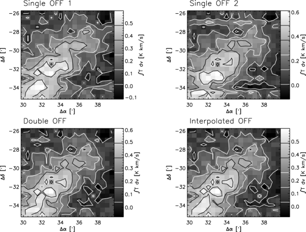
Figure 5: Channel map at 5.7 km/s obtained in the different calibration schemes from the same data as used for the integrated line maps in Fig. 3.

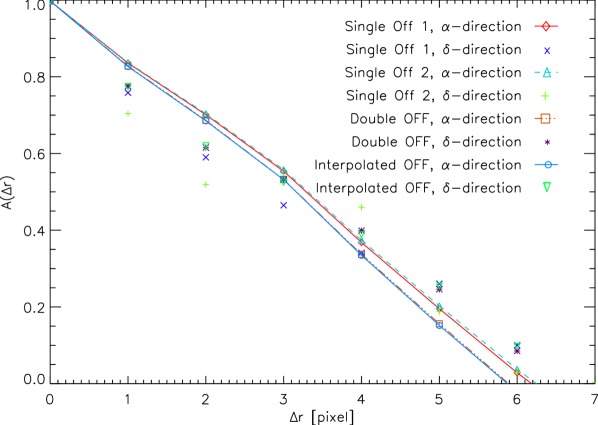
Figure 6: Autocorrelation function for the maps from Fig. 5 measured in the two perpendicular directions $\alpha$ and $\delta$.

The integrated line map discussed above is strongly susceptible to drift effects due to the short effective Allan time. To better study the effect of correlated radiometric noise we can use single channel maps where the radiometric noise is higher and the relative drift contribution is lower. An ideal observation would give a noise of $\sigma(t_{\rm tot})\approx 0.23$ K in this map. With the overheads quoted above this corresponds to 0.30 K radiometric noise per point and the maximum drift noise contribution $\sigma_{C,{\rm drift}}$ computed for the single-OFF calibration is only 0.44 $\sigma_{C,{\rm rad.}}$. Figure 5 shows the maps from the spectrometer channel at the peak of the average line profile obtained in the different calibration schemes. Figure 6 shows the corresponding autocorrelation functions measuring the anisotropy. We find, much smaller differences between the calibration schemes than in Fig. 3 but the differences are still dominated by drift effects and not by the different level of correlated radiometric noise. Those lines showing drift signatures in the integrated maps are the same lines that show the smaller deviations in the channel maps although the radiometric noise is higher in the channel maps. The channel maps are much more isotropic than the integrated line maps, but the maps calibrated by a single OFF still show noticeable stripes.

We can conclude that at least for maps with more that 10 pixels, the effect of correlated radiometric noise is small so that the choice of the calibration scheme should be based on the capability of correcting the drift of the system. The application of the different calibration schemes to real observations confirms the theoretical considerations that the single-OFF calibration is much more susceptible to drift effects than the other two calibration schemes so that it should be avoided. The example showed no significant advantage of the interpolated-OFF calibration relative to the double-OFF calibration. Both schemes lead to a strong reduction of the stripiness of the resulting maps.

5 Global optimization

5.1 Minimization of the total noise

For any given calibration scheme, the formalism introduced in Sect. 3.1 can also be used to optimize the actual timing of the observations. We can adapt the scanning speed of the OTF observations to provide source integration times resulting in a minimum uncertainty of the calibrated data.

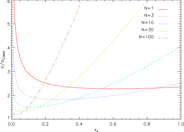
Figure 7: RMS of the total data uncertainty from radiometric and drift noise relative to the noise from an ideal instrument integrating the same total observing time. The noise is plotted as a function of the source point integration time relative to the Allan time for different numbers of points per scan, $N$. The interpolated-OFF calibration, a spectral index $\alpha=2.5$, and a dead time $x_{\rm d,1}+x_{\rm d,2}=0.25$ were used here.

This is demonstrated in Fig. 7 where the total data uncertainty is plotted as a function of the source integration time for different scan lengths when the interpolated-OFF calibration is used. A spectral index $\alpha=2.5$ typical of spectroscopic drifts and a total dead time of 0.25 Allan times were assumed here. The plot shows the maximum value across the OTF scans, which is typically reached at the ends of the scan for short cycles and in the center as soon as drift effects start to dominate.

For all scan lengths we find a characteristic minimum corresponding to the optimum source integration time. When using longer integration times, drift effects start to dominate. At shorter integration times, the relative overhead from the slew to and from the OFF position reduces the observing efficiency so that the radiometric noise is too high. We also see that the relative accuracy of the observations at the optimum timing grows with the scan size $N$. The equivalent plot for the double-OFF calibration shows a steeper increase of the noise when the source integration time is above its optimum value but minima which are slightly deeper than the minima shown here.

A special behavior occurs for very shallow spectra ($\alpha\la 0.75$). They show about the same slope at long integration times for all scan lengths so that the curves do not intersect. This means that very long scans are always favorable even if the resulting cycle length is much longer than the Allan time. This can be understood from the fact that in fluctuation spectra shallower than $1/f$, the noise is further reduced with increasing integration time, just like in the familiar case of white noise, but with another slope. The exact value for the transition to this behavior depends on the dead times involved but the limit $\alpha=0.75$ is a good approximation for most cases.

Independent from the spectral index of the fluctuations we find that the best observing mode is always given by very long scans with many points and a very short integration time per point in each scan. A full observation is obtained from many of these short-time coverages. This was already shown by Schieder & Kramer (2001). Unfortunately, there are always practical limitations to this approach. A telescope cannot move arbitrarily fast and the integrated data cannot be read out and dumped at an infinite data rate. Thus, the minimum relative integration time $x_{\rm min}$ set by the instrument is a limiting quantity for the optimum OTF timing. Moreover, the size of the astronomical source naturally constrains the scan size $N$. Small maps may consist of a limited number of points $N_{\rm max}$ only. For any given $x_{\rm min}$ and $N_{\rm max}$, a plot like Fig. 7, computed for the actual slewing time $x_{\rm d,1}+x_{\rm d,2}$, can be used to obtain the optimum setup. In most cases, the solution will still fall at the extreme provided by the maximum possible number of points and the minimum possible integration time.

At a number of ground-based telescopes (e.g. JCMT, MOPRA, KOSMA) the implemented OTF mode identifies the OTF scan length $N$ with the length of a single line in an OTF map $N_{\rm line}$. However, there is no a priori justification for this identity. In a more general approach, used e.g. at IRAM and APEX, multiple lines are combined within one OTF scan. An even more generalized approach is foreseen for the pointing mode definitions of the Herschel Space Telescope where an arbitrary number of points is measured between two OFF measurements, resulting in scan sizes that may cover also parts of map lines. This is partially motivated by the relatively slow slew to the OFF position by the telescope. Here, we consider this most general approach. When combining multiple map lines in one OTF scan the turn-around delay between subsequent lines, $t_{\rm turn}$, has to be taken into account when computing the total noise in the data. For a point $i$ measured within an OTF scan of length $N$, the number of turns before and after this point are $N_{\rm turn,1}=(i-1)/N_{\rm line}$ and $N_{\rm turn,2}=(N-i)/N_{\rm line}$, respectively. In Eq. (3.1), the total delay before the measurement $x_{\rm D,1}$ has to be increased by $N_{\rm turn,1}x_{\rm turn}$, the total delay after the measurement $x_{\rm D,2}$ by $N_{\rm turn,2}x_{\rm turn}$, and the total scan length $x_{\rm scan}$ by $(N_{\rm turn,1}+N_{\rm turn,2})x_{\rm turn}$ , where $x_{\rm turn}$ denotes the turn time relative to the Allan time, $x_{\rm turn}=t_{\rm turn}/t_{\rm A}$.

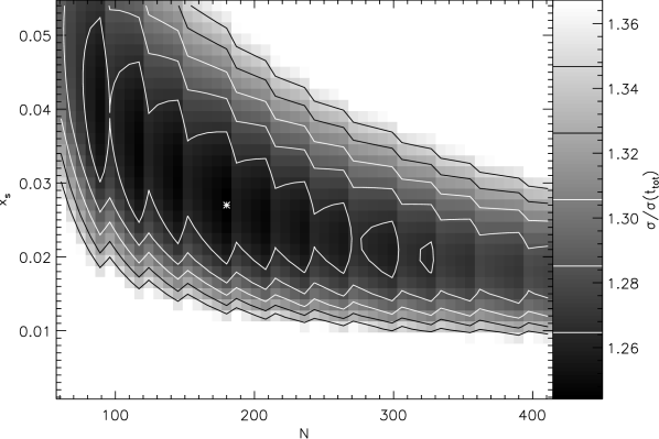
Figure 8: Relative RMS of the calibrated data in OTF observations as a function of the scan length and the integration time per source point relative to the system Allan time. Values of more than 10 % above the minimum are clipped in the plot. The asterisk marks the optimum setup resulting in the minimum noise at $N=180$ and $x_{\rm s}=0.028$. A line length of 30 points, an OFF dead time $x_{\rm d,1}+x_{\rm d,2}=0.6$, a turn time of the telescope $x_{\rm turn}=0.15$, and a spectral index $\alpha=2.5$ were used here.

In this case, the minimum of the relative data uncertainty is no longer found at the maximum scan length and the minimum possible integration time because of the increasing overhead for turns with increasing scan length. The optimization has to be done by actually evaluating Eq. (3.1) for different scan lengths and integration times. This is demonstrated in Fig. 8 showing the total noise RMS as a function of source integration time and scan length for a map where $N_{\rm line}=30$ and the relative inter-line overhead is $x_{\rm turn}=0.15$.

The most important feature in this plot is the large extent of the valley. Within the whole colored part of the plot, the noise RMS only changes by 10 % and even a 2 %-contour encloses a factor six in scan length and a factor two in the integration time. This means that OTF observations are extremely robust with respect to bad timings. Even in setups far from the optimum, the noise RMS is typically only enhanced by some ten percent. This explains why the OTF mode is used very successfully at many ground-based telescopes without a thorough theoretical analysis.

The staircase structure of the contours reflects turns which are added when the scan length exceeds multiples of the line length. We find several minima with their deepest points always at integer multiples of the line length. In this example, the absolute minimum falls at a scan length of 180 points, but scans with 90, 120, 150, or 210 points practically are not worse. In numerous tests with parameters typical of different telescopes we found no case with a minimum not falling at an integer multiple of full lines. Thus we can always complete lines in an OTF scan before going to the OFF position and it is typical that one can combine several lines in an OTF scan. To optimize actual observations, it is thus sufficient to evaluate Eq. (3.1) for scan sizes being integer multiples of the line length.

With the additional overhead given by the dead time between the OTF lines, the optimum source integration time is no longer automatically given by the minimum time allowed by the instrument. We find an optimum source integration time $x_{\rm s}$ between 0.02 and 0.04, corresponding to a full scan duration of about seven Allan times. This is a contradiction to the general wisdom, valid for symmetric observing modes, that the reference cycle period should be shorter than the Allan time. It can be easily explained by the fact, that the Allan time always compares radiometric and drift noise, but only a small fraction of the full period is used to integrate down the radiometric noise for any individual map point. However, this results in a general warning. To make sure that the proposed optimization scheme is actually valid, the Allan variance spectrum must not only be known up to a few Allan times, but it has to be determined over at least the time scale expected for the longest OTF observing cycles. This long term spectrum needs to be used the measure the stability time and to fit the drift power law to use the optimization formalism derived here.

Eq. (3.1) can also be used to check the optimum integration time for the OFF measurement. A rough estimate in Sect. 2.3 had shown that for the interpolated-OFF calibration scheme an OFF integration time of $t_{\rm OFF}=2/3\times\sqrt{N}t_{\rm s}$ should be sufficient. By introducing $q$ as a free parameter characterizing the relative OFF integration time $t_{\rm OFF}=q\sqrt{N}t_{\rm s}$ we can include it in the optimization. Searching for the global minimum in the three-dimensional parameter space spanned by $N$, $x_{\rm s}$, and $q$, we find an optimum value of $q=0.69$ for the parameters used in Fig. 8, a number that is close to the theoretical value from Sect. 2.3. The minimum is, however, very broad in the $q$-dimension so that the exact choice of the OFF time has hardly any influence on the total data uncertainty of the calibrated data. We find the same kind of robustness as for the scan lengths. Varying the model parameters showed that the optimum scan length depends strongly on the spectral index of the fluctuations, but that the optimum $q$-parameter is always close to 0.7. This value can be used for all observations applying the interpolated-OFF or the double-OFF scheme if the full integration time of both OFF measurements is used in the calibration.

Table 1: Examples for parameters of an optimum timing in an OTF map covering 30 points in each line. All values are given for a spectral resolution of 1 MHz, corresponding to a typical fluctuation bandwidth of 1.5 MHz.

observation	$t_{\rm A}$	$\alpha$	N	$t_{\rm s}$	$\sigma/\sigma(t_{\rm tot})$	$\sigma^{2}_{\rm drift}/\sigma^{2}_{\rm radio}$
	[s]			[s]
Ground-based telescope: $t_{s,{\rm min}}=1$ s, $t_{\rm d,1}+t_{\rm d,2}=20$ s, $t_{\rm turn}=8$ s
spectroscopic	80	2.5	180	2	1.17	0.07
total-power	8	1.5	60	1	1.70	0.70
HIFI at Herschel: $t_{s,{\rm min}}=1$ s, $t_{\rm d,1}+t_{\rm d,2}=80$ s, $t_{\rm turn}=20$ s
spectroscopic	150	2.5	180	4	1.23	0.10
total-power	10	1.5	150	1	2.13	1.03

To provide a feeling for the results, we give in Table 1 a few realistic examples. We compare the optimum timing and the resulting noise for typical parameters of a ground-based telescope and of the HIFI instrument at the Herschel Space Telescope. All values are given for a reference resolution of 1 MHz, which is typical of many high-frequency observation, but not for mm observations of Galactic sources. For such observations the numbers may only apply to binned or line-integrated data. Ground based telescopes have the general advantage that they can quickly slew to the OFF position and store the measured data at a high rate. Their big disadvantage is the atmospheric instability resulting in a relatively short Allan stability time for spectroscopic and continuum measurements. For HIFI observations with the Herschel Space Telescope we expect a more stable configuration, with an Allan time of about 150 s for spectroscopic drifts and of about 10 s for total-power drifts (see Sect. 1). On the other hand, all telescope slews are relatively slow so that we can estimate a slewing time of about 40 s when going to an OFF position which is 20^′ apart from the source.

For spectroscopic observations, being only sensitive to relative variations of the sensitivity across the spectrometer, we find in both cases an optimum scan length covering six full lines and $x_{\rm s,opt}\approx 0.025$ which translates into optimum integration times per source point of 2 s and 4 s, respectively. The full range of good observing parameters covers again scan lengths and integration times differing by up to a factor two from the optimum values. The drift contribution to the total noise is small in both cases, but the ground-based telescope is clearly superior in terms of the total noise per observing time due to the shorter dead times. For the Herschel observations the additional complexity of scanning subsequent lines in opposite directions is well justified because a limitation of the scan length to the line length would increase the optimum noise RMS by 9% corresponding to a 19% loss of observing efficiency. In observations for simultaneously determining the continuum level, where total-power drifts become relevant, the optimum integration time per source point falls below the 1 s minimum readout time for both configurations, so that the minimum time provided by the instrument has to be used. For a 1 s readout and the corresponding optimum scan length we find a significant drift contribution with an amplitude of 70 % of the radiometric noise for the ground-based example and 103 % for HIFI at Herschel. This means that the baseline uncertainty is as large as the radiometric noise contribution. The overall noise efficiency of the observations is low, relative to an ideal instrument we obtain 35 % for the ground-based and 22 % for the Herschel continuum observations. Using the OTF mapping mode for an accurate determination of the continuum level with heterodyne instruments is therefore questionable.

6 Discussion

One has to keep in mind that OTF observations in general and the optimization scheme proposed above in particular have a serious drawback. When reusing the calibrated data for purposes which were not foreseen when planning the observations, by spatial or spectral rebinning, the relative gain in the noise reduction is always lower than for pure radiometric noise. In spatial rebinning the contribution of the correlated noise from the OFF measurement stays constant (Beuther et al., 2000). By extending OTF scans over multiple lines of a map this effect is in principle even more enhanced. On the other hand, the total noise contribution from the OFF measurement drops with increased scan lengths so that the effect of correlated noise is also somewhat reduced by extending the scans. When applying the temporal optimization scheme the same becomes true for the spectral rebinning. The Allan time used to optimize the observations is determined by the ratio of drift noise and radiometric noise. Rebinning spectra to a coarser resolution only reduces the radiometric noise so that the relative contribution of the drift noise is enhanced.

Thus, OTF maps have always a limited use with respect to spatial of spectroscopic rebinning. In both cases artificial structures due to instrumental drifts or due to the correlated noise are enhanced. Consequently, a very careful planning of the observations has to be performed. The observer has to find a compromise between the efficiency of the observations and their re-usability. The optimization scheme should always be applied at the level of the coarsest spatial and spectral resolution that might be used for interpreting the calibrated data. The actual data taking can happen at a much higher spatial and spectral sampling. For the high sampling the observations will be less efficient, but the planning then guarantees that no artifacts will be produced by the foreseen smoothing. For example, if the observations are taken on a Nyquist sampled grid but a smoothing to a half-sampled grid, i.e. a reduction of the number of independent points by a factor four, is foreseen the OFF integration time should be approximately doubled compared to the case where the Nyquist sampling represents the spatial goal resolution. Then all artifacts from the observing mode are suppressed, however, at the costs of the observing efficiency. The more precise the scientific application of the measured data can be specified in terms of spatial and spectroscopic resolution the better can the actual observing scheme be adapted to the application resulting in more efficient observations.

7 Conclusions

In most cases mapping observations should follow the scheme known from OTF maps where the calibration of several source points uses a common OFF measurement for reference. This is far more efficient than all other reference modes. The efficiency can be further enhanced by combining multiple lines with one OFF measurement. This introduces, however, correlated noise across the calibrated map stemming from the common OFF integration. The impact of this correlated noise can be reduced by using the two neighboring OFF measurements as reference. Their optimum integration time is approximately $0.7\sqrt{N}t_{\rm s}$.

In most cases the calibration of the source data should follow the interpolated-OFF scheme where the data from both neighboring OFF measurements are weighted according to their temporal distance from the source measurement. This compensates all linear drifts of the instrument and results in the lowest total uncertainty of the calibrated data. The single-OFF calibration still used at several telescopes should be immediately abandoned because of the strong sensitivity of the calibrated data to drift effects. For short scans with less than 10 points at a fast telescope the double-OFF calibration is superior to the interpolated-OFF calibration. However, as soon as drift effects may become important, the robustness of the interpolated-OFF scheme turns it superior.

The total uncertainty of the calibrated data consisting of radiometric noise and drift noise can be computed when the fluctuation spectrum of instrumental instabilities is known, i.e. an Allan variance measurement was performed. For a known spectral goal resolution, the result can be used to optimize the time line for the actual realization of the mapping observations. It turns out that the OTF observing mode is in general very robust with respect to non-optimal timings. The scan length and the source integration time can be varied within a relatively broad range without increasing the total noise in the calibrated data by more than a few percent.

The optimization reveals some general relations on conditions for accurate and efficient mapping observations:

• The efficiency of all mapping modes grows with growing map size.

• The possibility of fast data readouts is in many cases essential to minimize the drift contributions.

• In most conditions OTF scans can consist of integer multiples of complete map lines.

The most essential impact on the data accuracy is provided by the system stability. All intervals have to be considered relative to the Allan time. The main prerequisite for any accurate mapping observation is thus a long instrumental stability, as measured by the Allan time. Due to the low gain stability of most heterodyne instruments it turns out that it is often impossible to derive significant information on the continuum level of astronomical sources using the OTF or raster mapping modes. They are always heavily influenced by the instrumental drifts.

Both the general design of the mapping modes with a common OFF measurement and the temporal optimization limit the re-usability of the data with respect to spatial or spectroscopic rebinning. The setup should be optimized with a clear picture of the resolution requirements set by the scientific goal of an observation.

Appendix A Effective beam broadening in OTF maps

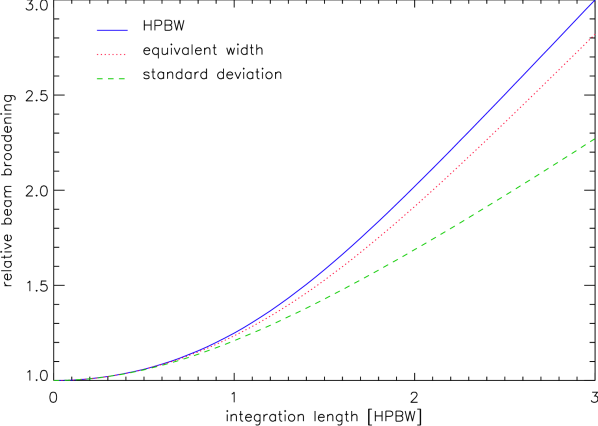
Figure 9: Beam broadening due to the scanning motion of the telescope during integration in OTF observations. The solid line shows the ratio between the HPBW of the effective beam in scanning direction and the original Gaussian beam. The dotted line represents the ratio between the corresponding equivalent widths and the dashed line the ratios of the standard deviations.

Often OTF observations are not be performed exactly on Nyquist sampling. Traditionally the difference between a sampling at half the beam width, HPBW/2, and a full Nyquist sampling is ignored by using the slightly coarser sampling. For a comparison of different tracers, it is moreover useful to map them at the same raster, even when the observation at different frequencies leads to a slightly different sampling with respect to the telescope beam. Thus it is very common to use samplings deviating from a full Nyquist sampling. We can compute the quantitative impact of the beam smearing in the general case by the numerical convolution of a two-dimensional Gaussian beam profile with a strip function of finite size representing the motion of the telescope during the integration. The result is shown in Fig. 9. The solid line shows the increase of the half-power beam width (HPBW) with increased integration length. We find that the beam broadening goes from the mentioned 4 % at the Nyquist sampling of 0.42 HPBW to 6 % at 0.5 HPBW and to 25 % at 1 HPBW. When using an integration length above 2 HPBW, the beam is completely dominated by the strip length. At 2 HPBW, the original beam contributes only by 2 %. The beam becomes less and less Gaussian. As a measure for the distortion of the beam shape we have also plotted the ratio between the standard deviation of the actual beam and the original beam. It grows much slower than the HPBW. The beam shape is close to Gaussian for scan lengths below 1 HPBW and almost rectangular above 2 HPBW. For an arbitrary beam shape the actual resolution is better described by the equivalent width of the beam, $\theta_{\rm eq}=\int P(\theta)d\theta/P_{\rm max}$, (Kraus, 1980). This is shown as dotted line in Fig. 9. It follows the curve for the HPBW for integration lengths below 1 HPBW, but is about 5 % lower at long integration lengths. The beam size perpendicular to the scanning direction is never affected by the OTF observing scheme.

Appendix B Signal correlations from power-law autocorrelation functions

Noise functions exhibiting a $1/f^{\alpha}$ power spectrum ($0<\alpha\leq 3,\alpha\neq 1$) are characterized by even power-law autocorrelation functions

$$\gamma(\tau)=g_{0}-g_{\alpha}|\tau|^{\alpha-1}\;.$$ (23)

The average correlation of the signal measured over a period $t_{1}$ with the signal measured over $t_{2}$ separated by an arbitrary delay $d$ can be computed as

$$\left\langle c_{1}(t)c_{2}(t)\right\rangle_{t} = {1\over t_{\rm 1}t_{\rm 2}}\int_{0}^{t_{\rm 1}}\!\!d\tau^{\prime}\int_{0}^{t_{2}}\!\!d\tau^{\prime\prime}\gamma(\tau^{\prime}-\tau^{\prime\prime}+d+t_{\rm s})$$

$$= {1\over t_{\rm 1}t_{\rm 2}}\int_{0}^{t_{\rm 1}}\!\!d\tau^{\prime}\int_{0}^{t_{2}}\!\!d\tau^{\prime\prime}\left(g_{0}-|\tau^{\prime}-\tau^{\prime\prime}+d+t_{\rm s}|^{\alpha-1}\right).$$

We can always chose $t_{1}$ to start before or at the same time as $t_{2}$, so that $t_{1}+d\geq 0$. Then we obtain

$$\left\langle c_{1}(t)c_{2}(t)\right\rangle_{t} = g_{0}-{1\over t_{\rm 1}t_{\rm 2}}\int_{0}^{t_{\rm 1}}d\tau^{\prime}{g_{\alpha}\over\alpha}\left[|\tau^{\prime}+d|^{\alpha}+(\tau^{\prime}+d+t_{\rm 1})^{\alpha}\right]$$ (25)

$$= g_{0}-{g_{\alpha}\over\alpha(\alpha+1)t_{\rm 1}t_{\rm 2}}\left[(t_{\rm 1}+t_{\rm 2}+d)^{\alpha+1}-(t_{\rm 1}+d)^{\alpha+1}\right.$$

$$\hskip 76.82234pt\left.-|t_{\rm 2}+d|^{\alpha+1}+|d|^{\alpha+1}\right]$$

The correlation between the signals measured in $t_{1}$ and $t_{2}$ decays basically with the total time spanned by the two integrations and the delay between them (first term in brackets), reduced by some corrections for the finite integration times.

One special case is the auto-correlation over the same time interval, i.e. $t_{1}=t_{2}=-d$. Then we obtain the simple expression

$$\left\langle c_{1}(t)^{2}\right\rangle_{t}=g_{0}-{2g_{\alpha}t_{\rm 1}^{\alpha-1}\over\alpha(\alpha+1)}\;.$$ (26)

Another important case is the correlation measured in Allan variance measurements with $t_{1}=t_{2}$, $d=0$. The correlation between two adjacent intervals of the same length is

$$\left\langle c_{1}(t)c_{2}(t)\right\rangle_{t}=g_{0}-{2g_{\alpha}(2^{\alpha}-1)t_{\rm 1}^{\alpha-1}\over\alpha(\alpha+1)}\;.$$ (27)

For the case of white noise, $\alpha=0$, Eq. (3.1) does not hold, but the correlation function represents a Dirac $\delta$-function, $\gamma(\tau)=g_{0}\delta(|\tau|)$. We obtain

$$\left\langle c_{1}(t)c_{2}(t)\right\rangle_{t} = {1\over t_{\rm 1}t_{\rm 2}}\int_{0}^{t_{\rm 1}}\!\!d\tau^{\prime}\int_{0}^{t_{2}}\!\!d\tau^{\prime\prime}\gamma_{0}\delta(\tau^{\prime}-\tau^{\prime\prime}+d+t_{\rm s})$$ (28)

$$= {g_{0}\over t_{\rm 1}t_{\rm 2}}\int_{0}^{t_{\rm 1}}\!\!d\tau^{\prime}\left\{\begin{array}[]{ll}1&\mbox{if $0\leq\tau^{\prime}\leq-d$}\\ 0&\mbox{otherwise}\end{array}\right.$$ (31)

$$= \left\{\begin{array}[]{ll}{-g_{0}d/(t_{\rm 1}t_{\rm 2})}&\mbox{if $d<0$}\\ 0&\mbox{otherwise}\end{array}\right.$$ (34)

This means that a noise correlation occurs only within the period of overlap of the two measurements given by the negative delay, $-d$. For all positive or zero delays, like in the Allan variance measurement, the correlation vanishes. The special case of the auto-correlation over the same time interval, leads to the well known radiometric noise behavior $\left\langle c_{1}(t)^{2}\right\rangle_{t}=g_{0}/t_{1}$.

Appendix C Raster map observations

Raster map observations differ from the OTF observations discussed in the main part of this paper by pointing individually at the different source map points instead of continuously scanning over the source. This has two effects. First, the effective beam of the observation is always equal to the actual telescope beam. It does not suffer from the beam broadening discussed for OTF maps in Sect. 1. Second, it introduces dead times between the observation of different points of a map. The observation of each source point is characterized by two time constants here, the source integration time $t_{\rm s}$ and the slew time to the next map position $t_{\rm m}$. For all points in the map, except for the last point of a scan, the total time needed for the measurement is given by $t_{\rm s,tot}=t_{\rm s}+t_{\rm m}$. No additional turn time between two map lines is required. If we redefine the slew time to the OFF position as $t_{\rm d,2}^{\prime}=t_{\rm d,2}-t_{\rm m}$ we can use all equations derived above for the calibration and the noise estimate in the OTF mode by using $t_{\rm s}$ whenever the integration time counts and $t_{\rm s,tot}$ whenever delays enter.

In particular the interpolation measure $l$ derived in Sect. 2.2 (Eq. 5) turns into

$$l={{t_{\rm R}/2+t_{\rm d,1}+(i-1/2)t_{\rm s,tot}}\over{t_{\rm R}+t_{\rm d,1}+t_{\rm d,2}^{\prime}+Nt_{\rm s,tot}}}$$ (35)

For the estimate of the total noise in the data Eq. (3.1) can still be used when the total delays include the additional slew times, i.e.

$$x_{\rm D,1} = x_{\rm d,1}+(i-1)x_{\rm s,tot}$$

$$x_{\rm D,2} = x_{\rm d,2}+(N-i)x_{\rm s,tot}=x_{\rm d,2}^{\prime}+(N-i)x_{\rm s,tot}+x_{\rm m}$$

$$x_{\rm scan} = x_{\rm d,1}+Nx_{\rm s,tot}+x_{\rm d,2}^{\prime}$$ (36)

The resulting general behavior corresponds to an OTF map with very long delays before and after the lines. The corresponding optimum timing may consist of scan lengths which are shorter than the line lengths but there are no qualitative differences to the properties discussed for OTF observations.

References

- Allan (1966) Allan, D.W. 1966, Proc. IEEE 54, no. 2, 221
- Ashdown et al. (2007) Ashdown, M-A.J.; Baccigalupi, C.; Balbi, A.; Bartlett, J.G.; Borrill, J. et al. 2007, A&A 467, 761
- Ball (1976) Ball, J.A. 1976, in Meeks M. (ed.): Methods of Experimental Physics, Vol. 12, Astrophysics, Part C, Radio Observations, Acad. Press, p. 55
- Bensch et al. (2001) Bensch, F.; Stutzki, J.; & Ossenkopf, V. 2001, A&A 366, 636
- Beuther et al. (2000) Beuther, H.; Kramer, C.; Deiss, B.; & Stutzki J. 2000, A&A 362, 1109
- Bunde & Havlin (1994) Bunde, A.; Havlin, S. 1994, Fractals in Science, Springer-Verlag, p. 64
- Emerson et al. (1979) Emerson, D.T.; Klein, U.; Haslam, C.G.T. 1979, A&A 76, 92
- Emerson & Gräve (1984) Emerson, D.T.; Gräve, R. 1984, A&A 190, 353
- Frisch (1995) Frisch, U. 1995, Turbulence, Cambridge Press, p. 54
- de Graauw & Helmich (2000) De Graauw, Th.; & Helmich F. 2000, in Pilbratt, G.L.; Cernicharo, J.; Heras, A.M.; Prusti T.; & Harris A. (eds.), “The Promise of the Herschel Space Observatory”, ESA SP-460, 45
- Kraus (1980) Kraus, J. 1980, Radio astronomy, Cygnus Quasar Books, Chapter 7
- Kutner & Ulich (1981) Kutner, M.L.; & Ulich, B.L. 1981, ApJ 250, 341
- Maino et al. (1999) Maino, D.; Burigana, C.; Maltoni, M.; Wandelt, B.D.; Górski, K.M. et al. 1999, A&ASS 140, 383
- Mangum et al. (2000) Mangum, J.G.; Emerson, D.T.; Greisen, E.W. 2000, in Imaging at Radio through Submillimeter Wavelengths, eds. J.G. Mangum, S.J.E. Radford, ASP Conf. Series 217, 179
- Ossenkopf (2002) Ossenkopf, V. 2002, “The HIFI intensity calibration framework”, ALMA-Memo 442
- Ossenkopf (2008) Ossenkopf V., 2008, A&A 479, 915, (paper I)
- Peitgen & Saupe (1988) Peitgen, H.-O.; Saupe, D. 1988, The Science of Fractal Images, Springer-Verlag, p. 65
- Reichertz et al. (2001) Reichertz, L.A.; Weferling, B.; Esch, W.; Kreysa, E. 2001, A&A 379, 735
- Rohlfs & Wilson (1986) Rohlfs, K.; Wilson, T.L. 1986, Tools of Radio Astronomy, Springer Berlin
- Schieder et al. (1985) Schieder, R.; Rau, G.; Vowinkel, B. 1985, in Instrumentation for Submillimetrer Spectroscopy, ed. E. Kollberg (Academic Press), 189
- Schieder & Kramer (2001) Schieder, R.; Kramer, C. 2001, A&A 373, 746
- Schieder et al. (1989) Schieder, R.; Tolls, V.; Winnewisser, G. 1998, Experimental Astronomy 1, no. 2, 101
- Schneider et al. (2006) Schneider, N.; Bontemps, S.; Simon, R.; Jakob, H.; Motte, F.; Miller, M.; Kramer, C.; Stutzki, J. 2006, A&A 458, 855
- Steer et al. (1984) Steer, D.G.; Dewdney, P.E.; Ito, M.R. 1984, A&A 137, 159