Random wetting transition on the Cayley tree :
a disordered first-order transition with two correlation length exponents

Abstract

We consider the random wetting transition on the Cayley tree, i.e. the problem of a directed polymer on the Cayley tree in the presence of random energies along the left-most bonds. In the pure case, there exists a first-order transition between a localized phase and a delocalized phase, with a correlation length exponent $\nu_{pure}=1$. In the disordered case, we find that the transition remains first-order, but that there exists two diverging length scales in the critical region : the typical correlation length diverges with the exponent $\nu_{typ}=1$, whereas the averaged correlation length diverges with the bigger exponent $\nu_{av}=2$ and governs the finite-size scaling properties. We describe the relations with previously studied models that are governed by the same “Infinite Disorder Fixed Point”. For the present model, where the order parameter is the contact density $\theta_{L}=l_{a}/L$ (defined as the ratio of the number $l_{a}$ of contacts over the total length $L$ ), the notion of “infinite disorder fixed point” means that the thermal fluctuations of $\theta_{L}$ within a given sample, become negligeable at large scale with respect to sample-to-sample fluctuations. We characterize the statistics over the samples of the free-energy and of the contact density. In particular, exactly at criticality, we obtain that the contact density is not self-averaging but remains distributed over the samples in the thermodynamic limit, with the distribution ${\cal P}_{T_{c}}(\theta)=1/(\pi\sqrt{\theta(1-\theta)})$.

I Introduction

In pure phase transitions, the approach to criticality is usually governed by a single correlation length exponent $\nu$ that describes all finite-size scaling properties. In the presence of frozen disorder however, the distribution of correlation functions may become very broad and disorder-averaged values can become atypical and dominated by rare events. This phenomenon has been first studied in one dimensional classical spin systems [1, 2, 3], where correlation functions can be expressed as product of random numbers, and have been then found in higher dimensional systems, such as the 2D random $q$-state Potts model [5] and the random transverse field Ising chain [4] (which is equivalent to the classical 2D McCoy-Wu model). It is important to stress that both the typical and averaged correlations are actually important, depending on the physical quantities one wants to study [1, 2, 4]. It turns out that close to a phase transition, the typical correlation length $\xi_{typ}$ and the disorder-averaged correlation length $\xi_{av}$ may have different critical behaviors. The best understood example is the random transverse field Ising chain, which has been studied in great detail by D.S. Fisher via a strong disorder renormalization approach [4] to obtain $\nu_{typ}=1$ and $\nu_{av}=2$. These two exponents $\nu_{typ}=1$ and $\nu_{av}=2$ also occur in other disordered models that are described by the same “Infinite Disorder Fixed Point” (see the review [6] and references therein). In the present paper, we present still another realization of this “Infinite Disorder Fixed Point” with $\nu_{typ}=1$ and $\nu_{av}=2$, as a random wetting transition on the Cayley tree.

Our physical motivation to consider such a model of random wetting on the Cayley tree was to better understand the similarities and differences with two other types of models involving directed polymers and frozen disorder :

(i) for the problem of the directed polymer in a random medium on the Cayley tree [7], there exists a freezing transition towards a low-temperature phase of finite entropy, where the polymer is essentially frozen along the random optimal path. Finite-size properties in the critical region [8, 9] have revealed the presence of two distinct correlation length exponents $\nu=2$ and $\nu^{\prime}=1$. In the random wetting model considered in the present paper, the difference is that the the random energies are not on all bonds of the Cayley tree, but only on the bonds of the left-most path, so that the phase transition corresponds to a freezing along this boundary path.

(ii) for the wetting [10] and Poland-Scheraga model of DNA denaturation [11] with a loop exponent $c>2$, where the corresponding pure transition is first-order, we have found numerically [12, 13] that in the presence of frozen disorder, the transition remains first order, but that two correlation length exponents $\nu_{typ}=1$ and $\nu=2$ appear. The random wetting model considered in the present paper corresponds to the limit of loop exponent $c\to\infty$ (since loops do not exist on the Cayley tree) of the model studied in Ref. [12] with the boundary conditions bound-unbound (see more details on the model in section 2.1 of Ref. [12]).

The paper is organized as follows. In Section II, we introduce the model and the interesting observables. In Section III, we discuss the statistical properties of the free-energy and conclude that the wetting transition remains first-order with a jump of the energy density. In section IV, we study the statistics of the attached and detached lengths, and give the consequences for the statistics of the order parameter in the critical region. We summarize our conclusions in VI. Appendix A contains for comparison the analysis of the properties of the wetting transition in the pure case. In Appendix B, we discuss the transition temperatures of the moments of the partition function in the disordered case.

II Model and observables

II.1 Definition of the model

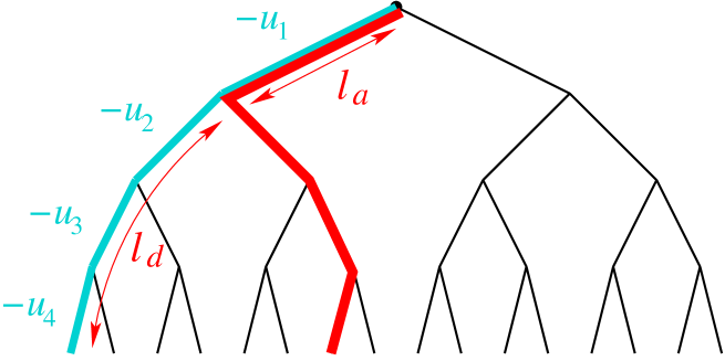
Figure 1: In this paper, we consider a Cayley tree of branching ratio $K$ and a number $L$ of generations ($K=2$ and $L=4$ on the Figure), and we study the statistical physics of a directed polymer starting at the root in the presence of random energies $(-u_{1},-u_{2},..,-u_{L})$ along the left-most bonds. A configuration of the directed polymer is characterized by an attached length $0\leq l_{a}\leq L$ along these left-most bonds and a detached length $l_{d}=L-l_{a}$ ($l_{a}=1$ and $l_{d}=3$ on the Figure). The delocalized phase corresponds to a finite $l_{a}$ as $L\to+\infty$, whereas the localized phase corresponds to a finite $l_{d}$ as $L\to+\infty$. The order parameter is the contact density $\theta=l_{a}/L$.

We consider a directed polymer of length $L$ on a Cayley tree of branching ratio $K$. The total number of directed walks is simply

$$Y_{L}=K^{L}$$ (1)

The corresponding delocalized free-energy reads

$$F_{L}^{deloc}\equiv-T\ln Y_{L}=-TL\ln K$$ (2)

and corresponds to an entropy of $(\ln K)$ per bond.

We now consider the random wetting model, where the left-most bonds are characterized by independent random energies $(-u_{i})$ with $i=1,2,..,L$ (see Figure 1). As an example, they can be drawn from the Gaussian distribution of average value $u_{0}>0$ and variance $\Delta^{2}$

$$p(u)=\frac{1}{\sqrt{2\pi\Delta^{2}}}e^{-\frac{(u_{i}-u_{0})^{2}}{2\Delta^{2}}}$$ (3)

II.2 Recurrence satisfied by the partition function

To write a recurrence for the partition function, it is convenient to label the random energies from the bottom, instead of the labelling from the root shown on Fig. 1

$${\tilde{u}}_{i}=u_{L-i}$$ (4)

The partition function $Z_{L}$ then satisfies the simple recurrence

$$Z_{L+1}=e^{\beta{\tilde{u}}_{L+1}}Z_{L}+(K-1)Y_{L}$$ (5)

with the initial condition $Z_{0}=1$. It is convenient to introduce the ratio with respect to the free partition function of Eq. 1

$$R_{L}\equiv\frac{Z_{L}}{Y_{L}}=\frac{Z_{L}}{K^{L}}$$ (6)

The recurrence then becomes

$$R_{L+1}=\frac{e^{\beta{\tilde{u}}_{L+1}}}{K}R_{L}+\frac{(K-1)}{K}$$ (7)

with the initial condition $R_{0}=1$.

II.3 Free-energy difference with the delocalized state

The difference between the free-energy $F_{L}=-T\ln Z_{L}$ and the delocalized free-energy of Eq. 2 is given by

$$F_{L}^{diff}\equiv F_{L}-F_{L}^{deloc}=-T\ln Z_{L}+T\ln Y_{L}=-T\ln R_{L}$$ (8)

The excess free-energy per monomer due to the wall in the thermodynamic limit $L\to+\infty$

$$f_{\infty}\equiv\mathop{\lim}_{L\to+\infty}\frac{F_{L}-F_{L}^{deloc}}{L}=-T\mathop{\lim}_{L\to+\infty}\frac{\ln R_{L}}{L}$$ (9)

characterizes the wetting transition : it vanishes in the delocalized phase $f_{\infty}(T>T_{c})=0$ and remains finite in the localized phase $f_{\infty}(T<T_{c})<0$.

II.4 Probability distributions of the attached length $l_{a}$ and of the detached length $l_{d}$

Since there is no loop on the Cayley tree, the directed polymer cannot return to the wall after leaving it. A configuration can be thus decomposed into a length $l_{a}$ attached to the wall starting at the root and a length $l_{d}=L-l_{a}$ detached from the wall (see Fig. 1). The thermal probability $Q_{L}(l_{a})$ to have exactly $l_{a}$ links attached to the wall in a given disordered sample reads

$$Q_{L}(l_{a})=\frac{e^{\displaystyle\beta\sum_{i=1}^{l_{a}}{u}_{i}}\left[\delta_{la,L}+(K-1)K^{L-l_{a}-1}\theta(l_{a}<L)\right]}{Z_{L}}$$ (10)

The numerator is the contribution to the partition function of the configurations that leave the wall after exactly $l_{a}$ steps. The denominator is the partition function

$$Z_{L}=\sum_{l_{a}=0}^{L}e^{\displaystyle\beta\sum_{i=1}^{l_{a}}{u}_{i}}\left[\delta_{la,L}+(K-1)K^{L-l_{a}-1}\theta(l_{a}<L)\right]$$ (11)

so that the normalization of the probability distribution $Q_{L}(l_{a})$ reads

$$\sum_{l_{a}=0}^{L}Q_{L}(l_{a})=1$$ (12)

It will be convenient to introduce also the probability distribution of the detached length $l_{d}=L-l_{a}$

$$P_{L}(l_{d})\equiv Q_{L}(l_{a}=L-l_{d})=\frac{e^{\displaystyle\beta\sum_{i=1}^{L-l_{d}}u_{i}}\left[\delta_{l_{d},0}+(K-1)K^{l_{d}-1}\theta(l_{d}\geq 1)\right]}{Z_{L}}$$ (13)

II.5 Order parameter : contact density

A convenient order parameter of the transition is the contact density, which is directly related to the attached length $l_{a}$ introduced in Eq. 10

$$\theta_{L}\equiv\frac{l_{a}}{L}$$ (14)

In particular, its thermal average in a given disordered sample is determined by the first moment of the distribution $Q_{L}(l_{a})$ of Eq. 10

$$<\theta_{L}>=\frac{<l_{a}>}{L}=\frac{1}{L}\sum_{l_{a}=0}^{L}l_{a}Q_{L}(l_{a})$$ (15)

In the thermodynamic limit $L\to\infty$, it is expected to remain finite in the localized phase and to vanish in the delocalized phase.

II.6 Internal Energy

The internal energy

$$E_{L}=-\partial_{\beta}\ln Z_{L}=-\partial_{\beta}\ln R_{L}$$ (16)

satisfies the recursion (see Eq. 7 for the corresponding recursion for the reduced partition function $R_{L}$)

$$E_{L+1}=\frac{e^{\beta{\tilde{u}}_{L+1}}R_{L}(-{\tilde{u}}_{L+1}+E_{L})}{e^{\beta{\tilde{u}}_{L+1}}R_{L}+(K-1)}$$ (17)

and the initial condition $E_{0}=0$. In terms of the attached length $l_{a}$ introduced above (see Eq. 10), it can also be written as

$$E_{L}=\frac{\displaystyle\sum_{l_{a}=0}^{L}\left(\displaystyle\sum_{i=1}^{l_{a}}u_{i}\right)e^{\displaystyle\beta\sum_{i=1}^{l_{a}}u_{i}}\left[\delta_{la,L}+(K-1)K^{L-l_{a}-1}\theta(l_{a}<L)\right]}{Z_{L}}$$ (18)

The energy per monomer in the thermodynamic limit $L\to+\infty$

$$e_{\infty}\equiv\mathop{\lim}_{L\to+\infty}\frac{E_{L}}{L}$$ (19)

remains finite in the localized phase $e_{\infty}(T<T_{c})>0$ and vanishes in the delocalized phase $e_{\infty}(T>T_{c})=0$. Its value can be obtained via the usual thermodynamic relation from the excess free-energy $f_{\infty}$ introduced in Eq. 9

$$e_{\infty}=\partial_{\beta}(\beta f_{\infty})$$ (20)

III Statistical properties of the free-energy

In this section, we discuss the statistics of the free-energy difference of Eq. 8 which depends only on the variable $R_{L}$ introduced in 6. We first explain that $R_{L}$ is a Kesten random variable and describe its statistical properties.

III.1 Analysis of the variable $R_{L}$ as a Kesten random variable

The recursion of Eq. 7 takes the form of the recurrence of Kesten variable [14]

$$R_{L+1}=a_{L+1}R_{L}+b$$ (21)

where $b=(K-1)/K$ is a constant and where the

$$a_{i}=\frac{e^{\beta u_{i}}}{K}$$ (22)

are independent identically distributed random variables. The specific structure of a Kesten variable $R_{L}$ consists in a sum of products of random variables

$$R_{L}=\prod_{i=1}^{L}a_{i}+b\left(1+\sum_{j=2}^{L}\prod_{i=j}^{L}a_{i}\right)$$ (23)

This discrete form has for continuous analog the exponential functional

$${\cal R}_{L}=\int_{0}^{L}dxe^{\int_{x}^{L}dyF(y)}$$ (24)

where $\{F(x)\}$ is the random process corresponding to the random variables $(\ln a_{i})$ in the continuous limit.

This type of random variables, either in the discrete or continuous forms, appears in a variety of disordered systems, in particular in random walks in random media [15, 16, 17, 18, 19, 20, 21, 22, 24, 25], in the classical random field Ising chain [26, 27], and in the quantum random transverse field Ising chain [28, 29, 30]. Many properties have been thus already studied in great detail in these previous works. In the following, we cite and translate these known results for the present context.

To describe the universal results near the critical point for large samples, there are only two relevant parameters :

(i) the first important parameter is the averaged value

$$F_{0}\equiv\overline{\ln a_{i}}=\beta\overline{u}-\ln K$$ (25)

The critical point corresponds to the vanishing condition $\overline{\ln a_{i}}=0$, so that the critical temperature of the present random wetting model reads

$$T_{c}=\frac{\overline{u}}{\ln K}$$ (26)

(In particular, for the Gaussian distribution of Eq. 3, the critical temperature is $T_{c}=u_{0}/(\ln K)$ and is independent of the variance $\Delta^{2}$.)

(ii) the second important parameter is the variance of $(\ln a_{i})$ that will be denoted by

$$2\sigma\equiv\overline{(\ln a_{i})^{2}}-(\overline{\ln a_{i}})^{2}=\beta\left(\overline{u_{i}^{2}}-(\overline{u_{i}})^{2}\right)$$ (27)

to keep the same notations as in Refs. [22, 25, 30]. In particular, from the Central Theorem, the sum $\Sigma_{N}=\displaystyle\sum_{i=1}^{N}(\ln a_{i})$ is then distributed asymptotically for large $N$ with the Gaussian distribution

$$P_{N}(\Sigma_{N})\mathop{\simeq}_{N\to\infty}\frac{1}{\sqrt{4\pi\sigma N}}e^{-\frac{(\Sigma_{N}-NF_{0})^{2}}{4\sigma N}}$$ (28)

III.2 Delocalized phase $T>T_{c}$

For $T>T_{c}$, the parameter of Eq. 25 is negative $F_{0}<0$ and the random variable $R_{L}$ remains a finite random variable as $L\to\infty$. Its probability distribution $P_{\infty}(R_{\infty})$ is known to display the power-law decay [14, 26, 27]

$$P_{\infty}(R_{\infty})\mathop{\propto}_{R_{\infty}\to\infty}\frac{1}{R_{\infty}^{1+\mu(T)}}$$ (29)

where the exponent $\mu(T)>0$ is determined by the condition

$$1=\overline{a^{\mu}_{i}}=\frac{\overline{e^{\mu\beta u_{i}}}}{K^{\mu}}$$ (30)

In conclusion, the difference of Eq. 8 between the free-energy $F_{L}$ and the delocalized free-energy $F_{L}^{deloc}$ remains a finite random variable as $L\to\infty$

$$F_{L}^{diff}\equiv F_{L}-F_{L}^{deloc}\mathop{\simeq}_{L\to\infty}F^{diff}\equiv-T\ln R_{\infty}$$ (31)

and its distribution presents the following exponential tail for $F_{diff}\to-\infty$ (see Eq. 29)

$$P_{deloc}(F^{diff})\mathop{\simeq}_{F_{diff}\to-\infty}e^{\beta\mu(T)F_{diff}}$$ (32)

Example : for the case of the Gaussian distribution of Eq. 3, the condition of Eq. 30 becomes

$$1=\frac{e^{\mu\beta u_{0}+\frac{\mu^{2}\beta^{2}\Delta^{2}}{2}}}{K^{\mu}}$$ (33)

and the exponent $\mu$ reads

$$\mu^{Gauss}(T)=\frac{2T(T\ln K-\overline{u_{L}})}{\Delta^{2}}=\frac{2(\ln K)T(T-T_{c})}{\Delta^{2}}$$ (34)

III.3 Critical point $T=T_{c}$

Exactly at criticality $T=T_{c}$, the parameter of Eq. 25 vanishes $F_{0}=0$. It is then known (see for instance [22, 23, 30] and references therein) that the leading behavior is of order

$$\ln R_{L}(T_{c})\mathop{\simeq}_{L\to\infty}2(\sigma L)^{1/2}w_{c}$$ (35)

where $w_{c}$ is a positive random variable of order $O(1)$. Moreover, it can be shown (see [30] and references therein) that the distribution of $w_{c}$ is the half-Gaussian distribution (cf Eqs (24) and (32) in [30])

$$P(w_{c})\simeq\theta(w_{c}\geq 0)\frac{2}{\sqrt{\pi}}e^{-w^{2}}$$ (36)

III.4 Localized phase $T<T_{c}$

For $T<T_{c}$, the parameter of Eq. 25 is positive $F_{0}>0$ and the random variable $R_{L}$ will grow exponentially in $L$

$$\ln R_{L}(T<T_{c})\mathop{\simeq}_{L\to\infty}LF_{0}+2\sqrt{\sigma L}w$$ (37)

The random variable $w$ of order $O(1)$ is distributed with the Gaussian distribution (cf Eqs (24) and (31) in [30])

$$P(w)\simeq\frac{1}{\sqrt{\pi}}e^{-w^{2}}$$ (38)

III.5 Summary of the critical behavior of the free-energy and energy

In conclusion, the difference of Eq. 8 between the free-energy $F_{L}$ and the delocalized free-energy $F_{L}^{deloc}$ displays the following critical behavior

$$F_{L}^{diff}(T>T_{c}) =F_{diff}\ \ {\rm of\ order}\ O(1)$$

$$F_{L}^{diff}(T_{c}) =-T_{c}2(\sigma L)^{1/2}w_{c}\ \ \ \ {\rm with}\ w_{c}>0\ {\rm of\ order}\ O(1)$$

$$F_{L}^{diff}(T<T_{c}) =-L(\overline{u}-T\ln K)-T2\sqrt{\sigma L}w\ \ \ \ {\rm with}\ w\ {\rm of\ order}\ O(1)$$ (39)

where the distributions of the random variables $F_{diff}$, $w_{c}$ and $w$ have been given above in Eqs 32, 36 and 38. In the thermodynamic limit $L\to+\infty$, the excess free-energy per monomer due to the wall defined in Eq. 9 is thus given by

$$f_{\infty}(T\geq T_{c}) =0$$ (40)

$$f_{\infty}(T\leq T_{c}) =-(\overline{u}-T\ln K)=-(T_{c}-T)\ln K$$ (41)

The thermodynamic relation of Eq. 20 then gives the behavior of the energy per monomer

$$e_{\infty}(T>T_{c}) =0$$ (42)

$$e_{\infty}(T<T_{c}) =-T_{c}\ln K=-\overline{u}$$ (43)

The transition is thus first-order, with a jump of the energy per monomer.

IV Statistical properties of the attached and detached lengths

In this section, we discuss the statistical properties of the attached length $l_{a}$ or of the complementary detached length $l_{d}$ whose distributions have been introduced in Eq. 10 and Eq. 13 respectively. This allows to analyse also the statistics of the contact density of Eq. 14, which represents the order parameter and of the internal energy of Eq. 18.

IV.1 Typical behavior of $Q_{L}(l_{a})$ in the delocalized phase

In the delocalized phase, the attached length $l_{a}$ will remain a finite random variable as $L\to\infty$. The typical decay of $Q_{L}(l_{a})$ is then given by (Eq. 10)

$$\overline{\ln Q_{L}(l_{a})} =\beta l_{a}\overline{u}+(L-l_{a})\ln K+\ln\frac{K-1}{K}-\overline{\ln Z_{L}}$$ (45)

$$\simeq-l_{a}(\ln K-\beta\overline{u})+\ln\frac{K-1}{K}+(L\ln K-\overline{\ln Z_{L}})$$

i.e. the decay is governed by the typical correlation length

$$\frac{1}{\xi_{typ}}=\ln K-\beta\overline{u}$$ (46)

that diverges with the correlation length exponent

$$\nu_{typ}=1$$ (47)

as in the pure case ( $\nu_{pur}=1$ of Eq. 87).

IV.2 Typical decay of $P_{L}(l_{d})$ in the localized phase

In the localized phase, the detached length $l_{d}$ will remain a finite random variable as $L\to+\infty$. The typical decay of $P_{L}(l_{d})$ is then given by

$$\overline{\ln P_{L}(l_{d})} =\beta(L-l_{d})\overline{u}+l_{d}\ln K+\ln\frac{K-1}{K}-\overline{\ln Z_{L}}$$ (49)

$$\simeq-l_{d}(\beta\overline{u}-\ln K)+\ln\frac{K-1}{K}+(L\beta\overline{u}-\overline{\ln Z_{L}})$$

i.e. the decay is governed by the typical correlation length

$$\frac{1}{\xi_{typ}}=\beta\overline{u}-\ln K$$ (50)

that diverges with the correlation length exponent

$$\nu_{typ}=1$$ (51)

as in the pure case ( $\nu_{pur}=1$ of Eq. 96).

IV.3 Statistics over the samples of the probability $q_{L}=Q_{L}(l_{a}=0)$ of zero contacts

To understand why typical and disordered averaged behaviors can be different for the distributions $Q_{L}(l_{a})$ and $P_{L}(l_{d})$, it is convenient to consider first the particular case of the probability of zero contacts

$$q_{L}\equiv Q_{L}(l_{a}=0)=P_{L}(l_{d}=L)=\frac{(K-1)K^{L-1}}{Z_{L}}=\frac{(K-1)}{K}\frac{1}{R_{L}}$$ (52)

because it depends only on the Kesten variable $R_{L}$ whose statistics has been discussed in detail in section III. We also note that $q_{L}$ coincides with the expression of the flux $J_{L}$ in the Sinai model, and we refer to [22] where many exact results have been derived for its probability distribution (see in particular Eq. (6.10) in [22]). In the following, we concentrate on the critical region. From the statistics of $R_{L}$ described in section III, one has in particular that

(i) in the delocalized phase, $q_{L}$ remains a finite random variable as $L\to+\infty$

(ii) in the localized phase, the probability $q_{L}$ becomes exponentially small in $L$

(ii) exactly at criticality, the variable $q_{L}$ behaves as $q_{L}\sim e^{-w_{c}2\sqrt{\sigma L}}$ where $w_{c}$ is a positive random variable of order $O(1)$ distributed with the half-Gaussian distribution of Eq. 36. As discussed in [30], an important consequence of the critical statistics of Eq.36 is that the averaged value is dominated by the rare samples having an anomalously small value of the scaling variable $0\leq w\leq 1/\sqrt{L}$, and since the probability distribution $P(w_{c})$ is finite at $w_{c}=0$, one obtains the slow power-law decay

$$\overline{q_{L}(T_{c})}\mathop{\propto}_{L\to\infty}\frac{1}{\sqrt{L}}$$ (53)

whereas the typical behavior is given by the exponential decay

$$\overline{\ln q_{L}(T_{c})}\mathop{\propto}_{L\to\infty}-\sqrt{L}$$ (54)

We refer to [30] and references therein for the discussion of similar examples of averaged values dominated by rare events in the field of quantum spin chains.

IV.4 Notion of “ Infinite Disorder Fixed Point”

The probability distribution $Q_{L}(l_{a})$ of the attached length $l_{a}$ in a given sample has the form of a Boltzmann measure

$$Q_{L}(l_{a})=\frac{e^{-U(l_{a})}}{\displaystyle\sum_{l_{a}=0}^{L}e^{-U(l_{a})}}$$ (55)

over the random walk potential

$$U(l_{a})=-\beta\sum_{i=1}^{l_{a}}{u}_{i}+l_{a}\ln K=-\sum_{i=1}^{l_{a}}\ln a_{i}$$ (56)

The continuum analog of Eq. 55 is then the Boltzmann measure over a Brownian potential (see Eq. 10 in [25]). We refer to [25] and references therein for more detailed discussions, but the essential property is that the Boltzmann measure over a Brownian valley is very concentrated (in a region of order $O(1)$) around the absolute minimum of the Brownian potential. Within our present notations, this means that in a given disordered sample at a given temperature, the thermal probability distribution $Q_{L}(l_{a})$ is concentrated in a finite region around the point $l_{a}^{*}$ where the random potential of Eq. 56 reaches its minimum on the interval $0\leq l_{a}\leq L$

$$Q_{L}(l_{a})\simeq\delta(l_{a}-l_{a}^{*})$$ (57)

This means that in a given sample, the contact density of Eq. 14 is essentially given by its thermal average

$$\theta_{L}\simeq<\theta_{L}>=\frac{l_{a}^{*}}{L}$$ (58)

IV.5 Sample-to-sample fluctuations of the contact density

We now discuss the sample-to-sample fluctuations of $l_{a}^{*}$ and of the contact density. The disorder average of the probability distribution $Q_{L}(l_{a})$ can be obtained as

$$\overline{Q_{L}(l_{a})}\simeq\overline{\delta(l_{a}-l_{a}^{*})}=\pi_{L}(l_{a})$$ (59)

where $\pi_{L}(l_{a}^{*})$ is the probability distribution of the minimum $l_{a}^{*}$ over the samples.

Taking into account the two parameters $F_{0}$ (Eq. 25) and $\sigma$ (Eq. 27) that characterize the large scale properties of the random walk $U(l_{a})$, the probability distribution $\pi_{L}(l_{a}^{*})$ of the minimum $l_{a}^{*}$ can be obtained as

$$\pi_{L}(l_{a}^{*})=\frac{\psi^{(F_{0})}(L-l_{a}^{*})\psi^{(-F_{0})}(l_{a}^{*})}{\int_{0}^{L}dl\psi^{(F_{0})}(L-l_{a}^{*})\psi^{(-F_{0})}(l_{a}^{*})}$$ (60)

where

$$\psi^{(F_{0})}(l)=\int_{0}^{+\infty}dUG^{(F_{0})}(U,l)$$ (61)

and where $G^{(F_{0})}(U,l)$ represents the probability for a biased random walk to go from $(0,0)$ to $(U,l)$ in the presence of an absorbing wall at $U=0^{-}$ (see for instance [30] for very similar calculations)

$$G^{(F_{0})}(U,l)=\frac{U}{2{\sqrt{\pi}}(\sigma l)^{3/2}}e^{-\frac{(U-F_{0}l)^{2}}{4\sigma l}}$$ (62)

The critical behavior can be analyzed as follows.

IV.5.1 Sample-to-sample fluctuations at criticality

At criticality where $F_{0}=0$, the function $\psi$ of Eq. 61 reads

$$\psi^{F_{0}=0}(l)=\int_{0}^{+\infty}dU\frac{U}{2{\sqrt{\pi}}(\sigma l)^{3/2}}e^{-\frac{U^{2}}{4\sigma l}}=\frac{1}{\sqrt{\pi\sigma l}}$$ (63)

The distribution of Eq. 60 for the position $l_{a}^{*}$ then reads

$$\overline{Q_{L}(l_{a}^{*})}=\pi_{L}^{(T_{c})}(l_{a}^{*})=\frac{1}{\pi\sqrt{l_{a}^{*}(L-l_{a}^{*})}}$$ (64)

As a consequence, we find that the contact density $\theta\simeq l_{a}^{*}/L$ is distributed at criticality over the samples with the law

$${\cal P}_{T_{c}}(\theta)=\frac{1}{\pi\sqrt{\theta(1-\theta)}}$$ (65)

IV.5.2 Sample-to-sample fluctuations in the delocalized phase

In the delocalized phase where $F_{0}<0$, the position $l_{a}^{*}$ of the minimum on $[0,L]$ of the Brownian potential of positive drift remains finite as $L\to+\infty$, and the probability distribution of Eq. 60 can be obtained as

$$\pi_{L}^{(T>T_{c})}(l_{a}^{*})\simeq_{L\to\infty}\frac{\psi^{(-F_{0})}(l_{a}^{*})}{\int_{1}^{+\infty}dl\psi^{(-F_{0})}(l)}$$ (66)

with

$$\psi^{(-F_{0})}(l_{a})=\int_{0}^{+\infty}dU\frac{U}{2{\sqrt{\pi}}(\sigma l_{a})^{3/2}}e^{-\frac{(U+F_{0}l_{a})^{2}}{4\sigma l_{a}}}=\frac{F_{0}^{2}(\sigma l_{a})^{1/2}}{\sigma^{2}2{\sqrt{\pi}}}\int_{0}^{+\infty}dzze^{-l_{a}\frac{F_{0}^{2}}{4\sigma}(1+z)^{2}}$$ (67)

In particular, it decays exponentially as

$$\overline{Q_{L}(l_{a})}=\pi_{L}^{(T>T_{c})}(l_{a})\mathop{\propto}_{l_{a}\to+\infty}\ e^{-\frac{F_{0}^{2}}{4\sigma}l_{a}}$$ (68)

with the correlation length

$$\xi_{a}=\frac{4\sigma}{F_{0}^{2}}\mathop{\propto}_{T\to T_{c}^{+}}\frac{1}{(T-T_{c})^{2}}$$ (69)

This should be compared with the typical decay of Eq. 45. As a consequence, the finite-size scaling properties in the critical region involves the correlation length exponent

$$\nu_{FS}=2$$ (70)

and not the typical correlation exponent that appears in Eq. 47.

IV.5.3 Sample-to-sample fluctuations in the localized phase

In the localized phase, where $F_{0}>0$, it is the detached length $l_{d}^{*}=L-l_{a}^{*}$ that remains finite as $L\to+\infty$, and the disorder-averaged probability of the detached length $l_{d}$ can be obtained as

$$\overline{P_{L}(l_{d})}=\pi_{L}^{(T<T_{c})}(l_{a}^{*}=L-l_{d}^{*})\simeq_{L\to\infty}\frac{\psi^{(F_{0})}(l_{d})}{\int_{1}^{+\infty}dl\psi^{(F_{0})}(l_{d})}$$ (71)

with

$$\psi^{(F_{0})}(l_{d})=\int_{0}^{+\infty}dU\frac{U}{2{\sqrt{\pi}}(\sigma l_{d})^{3/2}}e^{-\frac{(U+F_{0}l_{d})^{2}}{4\sigma l_{d}}}$$ (72)

In particular, it decays exponentially as

$$\overline{P_{L}(l_{d})}\mathop{\propto}_{l_{d}\to+\infty}\ e^{-\frac{F_{0}^{2}}{4\sigma}l_{d}}$$ (73)

with the correlation length

$$\xi_{d}=\frac{4\sigma}{F_{0}^{2}}\mathop{\propto}_{T\to T_{c}^{-}}\frac{1}{(T_{c}-T)^{2}}$$ (74)

This should be compared with the typical decay of Eq. 49. Again, this means that the finite-size scaling properties in the critical region are governed by the correlation length exponent $\nu_{FS}=2$ of Eq. 70.

V Discussion

V.1 Lack of self-averaging of the order parameter at criticality

Outside criticality, the contact density is self-averaging in the thermodynamic limit $L\to+\infty$

$${\cal P}_{T<T_{c}}(\theta) =\delta(\theta-1)$$ (75)

$${\cal P}_{T>T_{c}}(\theta) =\delta(\theta)$$ (76)

but exactly at criticality, we have obtained that the contact density $\theta$ remains distributed at criticality over the samples with the law of Eq. 65

$${\cal P}_{T_{c}}(\theta)=\frac{1}{\pi\sqrt{\theta(1-\theta)}}$$ (77)

The lack of self-averaging of densities of extensive thermodynamic observables at random critical points whenever disorder is relevant has been studied in [31, 32, 33]. The main idea is that off-criticality, self-averaging is ensured by the finiteness of the correlation function $\xi$, that allows to divide a big sample $L\gg\xi(T)$ into a large number of nearly independent sub-samples. However at criticality where the correlation length diverges $\xi=+\infty$, even big samples cannot be divided into nearly independent sub-samples, and one obtains a lack of self-averaging. The cases considered in [31, 32, 33] were second-order phase transitions, but the result of Eq. 65 means that the contact density is not self-averaging at the random first-order transition studied in this paper.

V.2 Physical interpretation of two correlation length exponents

The presence of two different correlation length exponents $\nu_{av}=2$ and $\nu_{typ}=1$ whenever the disorder is equivalent to a Brownian potential $U(x)$ is well known in other contexts, in particular for random walks in random media [19, 25], for the quantum transverse field Ising chain [4, 30] and more generally in other models described by the same “Infinite Disorder Fixed Point” (see the review [6] and references therein). The physical interpretation is the following [4] :

(i) the first length scale corresponds to the length $\xi_{typ}$ where the mean value $\overline{[U(L)-U(0)]}=F_{0}L$ is of order one, which yields

$$\xi_{typ}\sim\frac{1}{F_{0}^{\nu_{typ}}}\ \ \ {\rm with}\ \ \nu_{typ}=1$$ (78)

(ii) the second length scale corresponds to the length $\xi_{av}$ where most of the samples indeed have $(U(L)-U(0))\sim F_{0}L\pm\sqrt{\sigma L}$ of the same sign of the mean value, i.e. the scale $\sqrt{\sigma L}$ of the fluctuations should be of the same order of the mean value, which yields

$$\xi_{av}\sim\frac{1}{F_{0}^{\nu}}\ \ \ {\rm with}\ \ \nu_{av}=2$$ (79)

We have found that the finite-size scaling properties for disorder-averaged values over the samples are governed by $\nu_{FS}=\nu_{av}=2$ which actually saturates the general bound $\nu_{FS}\geq 2/d_{dis}$ [34], where $d_{dis}$ is the dimensionality of the disorder (here $d_{dis}=1$), whereas the typical exponent is smaller $\nu_{typ}=1$. This possibility of a first order transition that remains first order in the presence of quenched disorder has been already discussed in [34] and in Sec. VII A of Ref. [4].

VI Conclusions and perspectives

In this paper, we have studied the random wetting transition on the Cayley tree. We have obtained that the transition which is first order in the pure case, remains first-order in the presence of disorder, but that there exists two diverging length scales in the critical region : the typical correlation length diverges with the exponent $\nu_{typ}=1$, whereas the averaged correlation length diverges with the bigger exponent $\nu_{av}=2$ which governs the finite-size scaling properties over the samples. We have describe the relations with the previously studied models that are governed by the same “infinite disorder fixed point”. We have given detailed results on the statistics of the free-energy, and on the statistics of the contact density $\theta=l_{a}/L$ which constitutes the order parameter in wetting transitions. In particular, we have obtained that at criticality, the contact density is not self-averaging but remains distributed over the samples in the thermodynamic limit, with the distribution ${\cal P}_{T_{c}}(\theta)=1/(\pi\sqrt{\theta(1-\theta)})$.

As explained at the beginning, our physical motivation to consider such a model of random wetting on the Cayley tree was to better understand the similarities and differences with two other types of models involving directed polymers and frozen disorder described in the points (i) and (ii) of the Introduction. The results given in the present paper suggest the following conclusions :

(i) The freezing transition of the directed polymer in a random medium on the Cayley tree [7] is of a very different nature, since it is the exponent $\nu=2$ which governs the free-energy singular part (instead of $\nu_{typ}=1$ here). The appearance of a smaller exponent $\nu^{\prime}=1$ in some finite-size properties in the critical region [8, 9] should be then explained with another mechanism.

(ii) Let us now compare with the wetting and Poland-Scheraga model of DNA denaturation with a loop exponent $c>2$ that we have studied numerically in [12, 13]. We find that the random wetting model considered in the present paper ( that corresponds to the limit of loop exponent $c\to\infty$ of the model studied in Ref. [12] ) presents very similar critical behavior : in both cases, the transition remains first order with $\nu_{typ}=1$ and a finite contact density, but the finite-size scaling properties over the samples involve the exponent $\nu_{FS}=2$. We thus hope that the exact results obtained here for the special case $c\to\infty$ will help to better characterize the transition in the region of finite-loop exponent $2<c<+\infty$.

Appendix A Properties of pure wetting transition $u_{i}=u_{0}$

In this Appendix, we describe the critical properties of the pure wetting transition on the Cayley tree, to compare with the disordered case considered in the text.

A.1 Finite-size partition function

When all the energies $u_{i}$ take the same value $u_{0}$, the ratio $R_{L}$ of Eq. 6 simply reads

$$R_{L}^{pure} =\left(\frac{e^{\beta u_{0}}}{K}\right)^{L}+\frac{(K-1)}{K}\left[1+\left(\frac{e^{\beta u_{0}}}{K}\right)+\left(\frac{e^{\beta u_{0}}}{K}\right)^{2}+\dots+\left(\frac{e^{\beta u_{0}}}{K}\right)^{L-1}\right]$$ (80)

$$=\left(\frac{e^{\beta u_{0}}}{K}\right)^{L}+\frac{(K-1)}{K}\times\frac{\left(\frac{e^{\beta u_{0}}}{K}\right)^{L}-1}{\left(\frac{e^{\beta u_{0}}}{K}-1\right)}$$

The critical temperature $T_{c}$ then corresponds to the point where the energy per link $u_{0}$ exactly compensates the entropy per link $(\ln K)$ of the free walk

$$e^{\beta_{c}u_{0}}=K\ \ \to\ \ T_{c}^{pure}=\frac{u_{0}}{\ln K}$$ (81)

A.2 Delocalized phase $e^{\beta u_{0}}<K$

In the delocalized phase, the leading term of Eq. 80 remains finite

$$R_{L}^{pure}(T>T_{c})\mathop{\simeq}_{L\to\infty}\frac{(K-1)}{(K-e^{\beta u_{0}})}+...$$ (82)

and the excess free-energy per monomer due to the wall in the thermodynamic limit $L\to+\infty$ (Eq. 9) vanishes

$$f_{\infty}(T>T_{c})=0$$ (83)

The finite-size behavior of the full free-energy difference of Eq. 8 reads near criticality

$$F_{L}^{diff}(T>T_{c})=F_{L}(T>T_{c})-F_{L}^{deloc}=-T\ln R_{L}=-T\ln\frac{(K-1)}{(K-e^{\beta u_{0}})}\mathop{\simeq}_{T\to T_{c}^{+}}-T_{c}\ln\frac{1}{T-T_{c}}$$ (84)

In the delocalized phase, the probability distribution $Q_{L}(l_{a})$ of the attached length $l_{a}$ of Eq. 10 remains finite as $L\to\infty$

$$Q_{L}(l_{a})\equiv P_{L}(l_{d}=L-l_{a})\mathop{\simeq}_{L\to\infty}\left(1-\frac{e^{\beta u_{0}}}{K}\right)\left(Ke^{-\beta u_{0}}\right)^{-l_{a}}=Q_{\infty}(l_{a})$$ (85)

It decays exponentially

$$Q_{\infty}(l_{a})\mathop{\simeq}_{l_{a}\to+\infty}e^{-\frac{l_{a}}{\xi_{deloc}(T)}}$$ (86)

where the correlation length reads

$$\xi^{pure}_{deloc}(T>T_{c})=\frac{1}{u_{0}(\beta_{c}-\beta)}\mathop{\propto}_{T\to T_{c}^{+}}\frac{1}{(T-T_{c})^{\nu_{pure}}}\ \ {\rm with\ \ }\nu_{pure}=1$$ (87)

The thermally averaged contact density $<\theta_{L}>$ of Eq. 15 vanishes as

$$<\theta_{L}>\mathop{\simeq}_{L\to\infty}\frac{1}{L}\sum_{l_{a}=0}^{\infty}l_{a}Q_{\infty}(l_{a})=\frac{1}{L(Ke^{-\beta u_{0}}-1)}$$ (88)

i.e. in the critical region, it behaves as

$$<\theta_{L}>\mathop{\simeq}_{L\to\infty}=\frac{1}{L(\beta_{c}-\beta)}$$ (89)

A.3 Localized phase $e^{\beta u_{0}}>K$

In the localized phase $T<T_{c}^{pure}$, the leading term of the partition function of Eq. 80 is exponentially large in $L$

$$R_{L}^{pure}(T<T_{c})\mathop{\simeq}_{L\to\infty}\left(\frac{e^{\beta u_{0}}}{K}\right)^{L}\left[1+\frac{(K-1)}{\left(e^{\beta u_{0}}-K\right)}\right]+O(1)$$ (90)

The excess free-energy per monomer due to the wall in the thermodynamic limit $L\to+\infty$ (Eq. 9) reads

$$f_{\infty}(T<T_{c})=-(u_{0}-T\ln K)=-(T_{c}^{pure}-T)\ln K$$ (91)

i.e. it vanishes linearly as the temperature $T$ approaches the critical value $T_{c}^{pure}$. The transition is thus first order.

The internal energy of Eq. 16 becomes from Eq. 90

$$E_{L}(T<T_{c})\mathop{\simeq}_{L\to+\infty}-Lu_{0}+\frac{(K-1)u_{0}e^{\beta u_{0}}}{\left(e^{\beta u_{0}}-K\right)\left(e^{\beta u_{0}}-1\right)}+...$$ (92)

The intensive energy of Eq. 19 remains constant in the whole low-temperature phase

$$e_{\infty}(T<T_{c})=-u_{0}$$ (93)

and presents a jump at criticality.

The detached length $l_{d}$ remains a finite random variable in the thermodynamic limit $L\to\infty$ with the following distribution ( Eq. 13)

$$P_{\infty}(l_{d})=\frac{\delta_{l_{d}=0}+\theta(l_{d}\geq 1)\frac{K-1}{K}\left(\frac{e^{\beta u_{0}}}{K}\right)^{-l_{d}}}{\left[1+\frac{(K-1)}{K\left(\frac{e^{\beta u_{0}}}{K}-1\right)}\right]}$$ (94)

It decays exponentially

$$P_{\infty}(l_{d})\mathop{\simeq}_{l_{d}\to+\infty}e^{-\frac{l_{d}}{\xi(T)}}$$ (95)

where the correlation length diverges as

$$\xi^{pure}(T<T_{c})=\frac{1}{u_{0}(\beta-\beta_{c})}\mathop{\propto}_{T\to T_{c}^{-}}\frac{1}{(T_{c}-T)^{\nu_{pure}}}\ \ {\rm with\ \ }\nu_{pure}=1$$ (96)

A.4 Critical point $e^{\beta_{c}u_{0}}=K$

Exactly at criticality, the ratio of Eq. 80 reads

$$R_{L}^{pure}(T_{c})=1+\frac{(K-1)}{K}L$$ (97)

so that the free-energy difference is logarithmic in $L$

$$F_{L}^{diff}(T_{c})=F_{L}^{pure}(T_{c})-F_{L}^{deloc}(T_{c})=-T_{c}\ln R_{L}=-T_{c}\ln\left[1+\frac{(K-1)}{K}L\right]\mathop{\simeq}_{L\to\infty}-T_{c}\ln L$$ (98)

The recurrence of Eq. 17 for the energy becomes

$$E_{L+1}=\frac{KR_{L}}{KR_{L}+(K-1)}(-u_{0}+E_{L})=\frac{K+(K-1)L}{K+(K-1)(L+1)}(u_{0}+E_{L})$$ (99)

leading to

$$E_{L}^{pure}(T_{c})=-u_{0}\frac{KL+(K-1)\frac{L(L-1)}{2}}{K+(K-1)L}=-u_{0}\frac{(L-1)}{2}\times\frac{1+\frac{2K}{(K-1)(L-1)}}{1+\frac{K}{(K-1)L}}$$ (100)

so that the energy per monomer in the thermodynamic limit $L\to\infty$ is

$$e_{\infty}^{pure}(T_{c})=-\frac{u_{0}}{2}$$ (101)

i.e. exactly in the middle of the jump between $e_{\infty}^{pure}(T<T_{c})=-u_{0}$ (Eq. 93) and $e_{\infty}^{pure}(T>T_{c})=0$.

The probability distribution $Q_{L}(l_{a})$ of the attached length $l_{a}$ for a system of size $L$ becomes at criticality

$$Q_{L}(l_{a})=\frac{\left[\delta_{l_{a},L}+\frac{(K-1)}{K}\theta(l_{a}<L)\right]}{1+\frac{(K-1)}{K}L}$$ (102)

i.e. it is essentially flat over all values $0\leq l_{a}\leq L$. The two phases coexist with proportions $(l_{a},l_{d}=L-l_{a})$. So the value of Eq. 100 simply means that the domain wall between the two phases is on average at the middle $(l_{a}=l_{d}=L/2)$, but the domain wall is actually anywhere on the interval $0\leq l_{a}\leq L$ with a flat distribution.

Appendix B Disordered case : transition temperatures $T_{n}$ for the averaged moments $\overline{Z_{L}^{n}}$ of the partition function

Since in other disordered models, one sometimes consider the series $T_{n}$ of critical temperatures for the moments $\overline{Z_{L}^{n}}$ of the partition function, we discuss their properties in the present Appendix. For $n=1$, one sees that the annealed partition function satisfies the recursion (see Eq. 7)

$$\overline{R_{L+1}}=\frac{\overline{e^{\beta u}}}{K}\overline{R_{L}}+\frac{(K-1)}{K}$$ (103)

This is equivalent to the pure case recursion with the change $e^{\beta u_{0}}\to\overline{e^{\beta u}}$ so that the annealed critical temperature is determined by the condition (see Eq. 81)

$$\overline{e^{\beta_{1}u}}=K$$ (104)

i.e. in terms of the exponent $\mu(T)$ introduced in Eq. 30, this corresponds to the condition

$$\mu(T_{1})=1$$ (105)

More generally from the power-law of Eq. 29, it is clear that the transition temperature $T_{n}$ for the moments $\overline{Z_{l}^{n}}$ of order $n$ is determined by the condition

$$\mu(T_{n})=n$$ (106)

For instance, for the case of the Gaussian distribution of Eq. 3, the expression of Eq. 34 yields

$$T_{n}=T_{c}\frac{1+\sqrt{1+2n\frac{\Delta^{2}}{T_{c}^{2}\ln K}}}{2}$$ (107)

References

• [1] B. Derrida and H. Hilhorst, J. Phys. C14, L539 (1981).
• [2] A. Crisanti, G. De Simone, G. Paladin and A. Vulpiani, Physica A192, 589 (1993).
• [3] J.M. Luck, “Systèmes désordonnés unidimensionnels”, Aléa Saclay (1992) and references therein.
• [4] D. S. Fisher Phys. Rev. Lett. 69, 534-537 (1992); D. S. Fisher Phys. Rev. B 51, 6411-6461 (1995).
• [5] A.W.W. Ludwig, Nucl.Phys. B330, 639 (1990)
• [6] F. Igloi and C. Monthus, Phys. Rep. 412, 277 (2005).
• [7] B. Derrida and H. Spohn, J. Stat. Phys., 51, 817 (1988).
• [8] J. Cook and B. Derrida, J. Stat. Phys. 63, 505 (1991).
• [9] C. Monthus and T. Garel, Phys. Rev. E 75, 051119 (2005).
• [10] M. E. Fisher, J. Stat. Phys. 34, 667 (1984).
• [11] D. Poland and H.A. Scheraga eds., Academic Press, New York (1970)
“Theory of Helix-Coil transition in Biopolymers”.
• [12] T. Garel and C. Monthus, J. Stat. Mech. P06004 (2005).
• [13] C. Monthus and T. Garel, Eur. Phys. J. B 48, 393 (2005).
• [14] H. Kesten, M. Koslov and F. Spitzer, Composio. Math. 30 (1975) 145.
• [15] F. Solomon, Ann. Prob. 3 (1975) 1.
• [16] Y. Sinai, Theor. Prob. Appl. 27 (1982) 256.
• [17] B. Derrida and Y. Pomeau, Phys. Rev. Lett 48, 627 (1982) ; B. Derrida, J. Stat. Phys. 31, 433 (1983).
• [18] V. Afanasev, Theor. Prob. Appl. 35, 205 (1990).
• [19] J. P. Bouchaud, A. Comtet, A. Georges and P. Le Doussal, Ann. Phys. 201, 285(1990).
• [20] S. F. Burlatsky, G. S. Oshanin, A. V. Mogutov, and M. Moreau Phys. Rev. A 45 , R6955 (1992).
• [21] G. Oshanin, A. V. Mogutov and M. Moreau, J. Stat. Phys. 73 , 379 (1993).
• [22] C. Monthus and A. Comtet, J. Phys. I (France) 4, 635 (1994).
• [23] A. Comtet, C. Monthus and M. Yor, J. Appl. Prob. 35, 255 (1998).
• [24] D.S. Fisher, P. Le Doussal and C. Monthus, Phys. Rev. Lett. 80 3539 (1998); P. Le Doussal, C. Monthus, D.S. Fisher, Phys. Rev. E 59 4795 (1999).
• [25] C. Monthus and P. Le Doussal, Phys. Rev. E 65, 066129 (2002).
• [26] B. Derrida and H.J. Hilhorst, J. Phys. A 16, 7183 (1983).
• [27] C. Calan, J.M. Luck, T. Nieuwenhuizen and D. Petritis, J. Phys. A 18 (1985) 501.
• [28] F. Igloi and H. Rieger. Phys. Rev. B 57, 11404 (1998).
• [29] A. Dhar and A.P. Young, Phys. Rev. B 68, 134441 (2003).
• [30] C. Monthus, Phys. Rev. B 69, 054431 (2004).
• [31] S. Wiseman and E. Domany, Phys Rev E 52, 3469 (1995).
• [32] A. Aharony, A.B. Harris, Phys Rev Lett 77, 3700 (1996).
• [33] S. Wiseman and E. Domany, Phys. Rev. Lett. 81 22 (1998) and Phys Rev E 58 2938 (1998).
• [34] J. T. Chayes, L. Chayes, D.S. Fisher and T. Spencer Phys. Rev. Lett. 57, 2999 (1986).