Matter fields near quantum critical point in (2+1)-dimensional U(1) gauge theory

Abstract

We study chiral phase transition and confinement of matter fields in (2+1)-dimensional U(1) gauge theory of massless Dirac fermions and scalar bosons. The vanishing scalar boson mass, $r=0$, defines a quantum critical point between the Higgs phase and the Coulomb phase. We consider only the critical point $r=0$ and the Coulomb phase with $r>0$. The Dirac fermion acquires a dynamical mass when its flavor is less than certain critical value $N_{f}^{c}$, which depends quantitatively on the flavor $N_{b}$ and the scalar boson mass $r$. When $N_{f}<N_{f}^{c}$, the matter fields carrying internal gauge charge are all confined if $r\neq 0$ but are deconfined at the quantum critical point $r=0$. The system has distinct low-energy elementary excitations at the critical point $r=0$ and in the Coulomb phase with $r\neq 0$. We calculate the specific heat and susceptibility of the system at $r=0$ and $r\neq 0$, which can help to detect the quantum critical point and to judge whether dynamical fermion mass generation takes place.

1 Introduction

Quantum electrodynamics in (2+1)-dimensional space-time has wide applications in a number of planar strongly correlated systems, including fractional quantum Hall system, Heisenberg quantum antiferromagnet, and high-$T_{c}$ cuprate superconductor. Among its numerous variants, the massless spinor QED₃ and the $\mathrm{CP}^{N}$ model are particularly interesting. They both exhibit fruitful physics in the context of quantum field theory and have proved to be powerful in understanding some fundamental physics of cuprate superconductors.

It is widely accepted that the $t$-$J$ model captures the essential physics of cuprate superconductors [1]. However, it is far from clear how to treat this model by satisfactory analytic tools. One frequently used approach to deal with the $t$-$J$ model is based on the slave-particle technique [1]. For example, the electron operator on $i$-lattice $c_{i}$ can be decomposed as

$$c_{i}=f_{i}b_{i}^{\dagger},$$ (1)

where $f_{i}$ represents the operator of spin-carrying spinon and $b_{i}^{\dagger}$ represents the charge-carrying holon. Such decomposition has a redundancy since the electron operator is invariant under the transformations

$$f_{i}\rightarrow e^{i\theta}f_{i},\,\,\,b_{i}\rightarrow e^{i\theta}b_{i},$$ (2)

which can be considered as an emergent gauge symmetry. This emergent gauge structure has very important effects on the whole physical picture and has been investigated extensively for twenty years [1, 2, 3, 4, 5, 6]. However, such decomposition is not unique and one can alternatively use the so-called slave-fermion approach, in which the spin quantum number is carried by scalar field [7] and the gauge charge is carried by fermionic matter field [8].

Recently, a new state of matter, named as algebraic charge liquid, was proposed to describe the low-energy properties of cuprate superconductors [8, 9]. The effective field theory of this state consists of $N_{f}$-flavor massless Dirac fermions, $N_{b}$-flavor scalar bosons, and a U(1) gauge field. This effective theory can be loosely considered as a combination of massless spinor QED₃ and $\mathrm{CP}^{N_{b}-1}$ model [9]. It has been used to understand certain quantum phase transitions and various exotic properties near the quantum critical points [8, 9]. Recently, this model was studied by Kaul and Sachdev [9] with emphasis put on the anomalous dimensions and some observable thermodynamic quantities including specific heat and susceptibility near the quantum critical point between Higgs and Coulomb phases.

When interacting with U(1) gauge field, there is an interesting possibility that the massless Dirac fermion might undergo a vacuum condensation, which then generates a finite mass for Dirac fermion [10, 11, 12]. This mass breaks the continuous chiral symmetry possessed by Dirac fermions and leads to new phenomena. Another characteristic property of QED₃ is that the strong gauge field can confine the matter fields that carry nonzero gauge charges [13, 14]. In the absence of scalar field, it is found that the fermion mass can be generated only for flavor $N_{f}<N_{f}^{c}\approx 3.3$ [10], and confinement takes place once the mass is generated [14]. If the gauge field also couples to the scalar field $z$, then the phenomena related to chiral phase transition and confinement will be modified by the dynamics of scalar bosons.

In this paper, we study chiral phase transition and confinement of matter fields in the vicinity of the quantum critical point. The critical fermion flavor $N_{f}^{c}$ depends on two parameters: the scalar boson flavor $N_{b}$ and the scalar boson mass $r$. When $r>0$, the system stays in the Coulomb phase, while $r=0$ defines the quantum critical point that separates the Coulomb phase from the Higgs phase. When the chiral symmetry is dynamically broken, the massless fermions become massive and are confined if $r\neq 0$; while the Dirac fermions and $z$ bosons are deconfined at the quantum critical point $r=0$. Since the confined and deconfined matter fields behave quite differently, the Coulomb phase and the critical point have completely different low-energy elementary excitations. Thus it is possible to specify the quantum critical point and to verify whether the chiral symmetry is dynamically broken by measuring observable physical quantities such as specific heat and susceptibility. We calculate these quantities within the effective gauge theory and discuss their behaviors at low temperature.

The paper is organized as follows. We study the dynamical mass generation for Dirac fermions in Section 2. The confinement/deconfinement properties of matter fields is discussed in Section 3. We then calculate the specific heat and susceptibility at quantum critical point $r=0$ in Section 4 and in the Coulomb phase with $r\neq 0$ in Section 5. The last section contains summary and discussion.

2 Dynamical fermion mass generation for $r\geq 0$

The action for the interaction between massless Dirac fermion and U(1) gauge field is

$$\mathcal{S}_{f}=\frac{1}{4}\int d^{3}xF_{\mu\nu}F^{\mu\nu}+\sum_{i}\int d^{3}x\overline{\psi}_{i}\gamma^{\mu}\left(\partial_{\mu}-ia_{\mu}\right)\psi_{i},$$ (3)

where the fermion has $N_{f}$ flavor. The spinor field $\psi$ describes the superconducting quasiparticle that carries physical electric charge. Here, for generality we keep the kinetic term of gauge field. Following Kaul and Sachdev [9], we consider only non-compact gauge field and omit the instanton excitations, so the above field theoretic model might not precisely match the low-lying theory of cuprate superconductors (there are theoretical and simulation evidence for the irrelevance of instantons in the presence of massless Dirac fermions with sufficiently large flavor $N_{f}$ [15, 16, 17]). In order to define chiral symmetry, we adopt a four-component representation of spinor field $\psi$ and three $4\times 4$ matrices $\gamma_{\mu}$ ($\mu=0,1,2$) satisfying the Clifford algebra, $\{\gamma_{\mu},\gamma_{\nu}\}=2\delta_{\mu\nu}$. Since the fermions are massless, the action $\mathcal{S}_{f}$ respects the following continuous chiral symmetry

$$\psi\rightarrow e^{i\varphi\gamma_{3,5}}\psi,$$ (4)

with $\gamma_{3}$ and $\gamma_{5}$ being two $4\times 4$ matrices that anticommute with $\gamma_{\mu}$. The action contains no small coupling constant and generally can only be treated using the $1/N_{f}$ expansion.

The free propagator for Dirac fermion is

$$G_{0}^{-1}(p)=i\gamma_{\mu}p^{\mu}.$$ (5)

The interaction with gauge field modifies it into the complete fermion Green function

$$G^{-1}(p)=i\gamma_{\mu}p^{\mu}+\Sigma(p),$$ (6)

where $\Sigma(p)$ is the fermion self-energy function. Generically, the fermion self-energy can be written as

$$\Sigma(p)=i\gamma_{\mu}p^{\mu}(A(p^{2})-1)+B(p^{2}),$$ (7)

with $A(p^{2})$ being the wave functional renormalization and $B(p^{2})$ the fermion mass function. To calculate the fermion self-energy, we can use either conventional perturbation expansion method or non-perturbative approach. If the usual perturbation theory is used, then the self-energy function is proportional to $\sim\eta\gamma\cdot p\ln(p)$ to the leading order of $1/N_{f}$ expansion [6, 9], which represents only a correction to the wave function (field operator). When combined with the free propagator $i\gamma_{\mu}p^{\mu}$, this self-energy modifies the fermion propagator to a new form

$$G(p)=\frac{i\gamma_{\mu}p^{\mu}}{p^{2-2\eta}},$$ (8)

which reflects the typical behavior of algebraic charge/spin liquid [6, 9]. This result implies that, to the leading order, the gauge fluctuation is only a marginal perturbation and no mass term $B(p^{2})$ is generated. In fact, such mass term can never be generated to any finite order of perturbative expansion. This can be understood by the symmetry arguments. Both the free action (3) and the term $i\gamma_{\mu}p^{\mu}A(p^{2})$ are chiral symmetric, but the mass term $B(p^{2})$ is not chiral symmetric. Therefore, it is the chiral symmetry of the action that prevents the occurrence of mass term $B(p^{2})$.

Figure 1: The solid line represents the propagator of Dirac fermions, dashed line the scalar boson $z$, and dotted line the field $\lambda$. (a) and (b) correspond to the polarization function from $z$ bosons. (c) corresponds to the polarization function from Dirac fermions. (d) corresponds to the polarization of field $\lambda$.

However, the perturbation theory can not tell us everything. Although the action is chiral symmetric, it is possible that its ground state does not respect the chiral symmetry and the Dirac fermion acquires a finite dynamical mass. Indeed, the generation of nonzero $B(p^{2})$ signals the happening of a phase transition and the reconstruction of the ground state, which are surely non-perturbative in nature and can not be analyzed by ordinary perturbation theory. The standard non-perturbative approach to the problem of dynamical fermion mass generation is to solve the Dyson-Schwinger (DS) equation for the fermion mass function, which was originally proposed by Nambu and Jona-Lasinio in the context of particle physics [18]. The DS equation can be written in the form

$$G^{-1}(p)=G_{0}^{-1}(p)-\int\frac{d^{3}k}{(2\pi)^{3}}\gamma_{\mu}G(k)\Gamma_{\nu}(p,k)D_{\mu\nu}(p-k),$$

where $\Gamma_{\nu}(p,k)$ is the vertex function and $D_{\mu\nu}(p-k)$ the photon propagator. After a series of manipulations, the above equation is decomposed into a couple of equations for $A(p^{2})$ and $B(p^{2})$ respectively

$$A(p^{2}) = 1+\frac{1}{4p^{2}}\int\frac{d^{3}k}{(2\pi)^{3}}\mathrm{Tr}[\gamma\cdot k\gamma_{\mu}G(k)\Gamma_{\nu}D_{\mu\nu}(p-k)],$$

$$B(p^{2}) = -\frac{1}{4}\int\frac{d^{3}k}{(2\pi)^{3}}\mathrm{Tr}[\gamma_{\mu}G(k)\Gamma_{\nu}D_{\mu\nu}(p-k)].$$

If the DS equation for $B(p^{2})$ has only vanishing solution, the fermions remain massless and are stable against gauge fluctuations. Whenever the equation develops a nontrivial solution $B(p^{2})$, the massless fermion acquires a finite mass. The crucial difference between the perturbative and non-perturbative approaches is that the DS equation is nonlinear which makes it possible for chiral phase transition to happen at the bifurcation point.

The logic presented above is analogous to the gap generation for fermion excitations in the BCS theory of conventional superconductors. In a normal metal, when we compute the mean value $\langle c_{k\uparrow}c_{-k\downarrow}\rangle$ using ordinary perturbative expansion, only vanishing result can be obtained. It could be understood that the local gauge symmetry of the system prevents the appearance of nonzero $\langle c_{k\uparrow}c_{-k\downarrow}\rangle$ which is not gauge invariant. However, a finite gap can be obtained by solving the nonlinear gap equation that is constructed by non-perturbative approach. Apparently, the local gauge symmetry does not prevent the gap generation; on the contrary, this symmetry is spontaneously broken by the finite gap since $\langle c_{k\uparrow}c_{-k\downarrow}\rangle\neq 0$. The gap generation signals a phase transition from normal metal to superconductor. In fact, the idea of dynamical fermion mass generation was motivated by the Cooper pairing picture in BCS theory [18]. The order parameter for chiral phase transition is just the fermion mass term $\langle\bar{\psi}\psi\rangle$ which is caused by fermion vacuum condensation.

For the spinor QED model (3), the chiral phase transition has been studied for many years. It is known that there exists a critical fermion flavor $N_{f}^{c}$ which separates the chiral symmetric phase ($N_{f}>N_{f}^{c}$) from the chiral symmetry broken ($N_{f}<N_{f}^{c}$) phase [10, 11, 12]. The critical flavor is about $N_{f}^{c}\approx 3.3$ to the leading order of $1/N_{f}$ expansion [10].

We now add the action of complex scalar field. At half-filling, the cuprate superconductor is a Mott insulator with long-range Neel order. The Neel order parameter $\mathbf{n}$ can be represented by the scalar boson operator $z_{\alpha}$ by

$$\mathbf{n}=z_{\alpha}^{\ast}\mathbf{\sigma}_{\alpha\beta}z_{\beta}.$$ (9)

Then the Neel state can be described by an effective field theory called $\mathrm{CP}^{N_{b}-1}$ model, where $N_{b}$ is the flavor of scalar field $z_{\alpha}$. This model admits an emergent local gauge symmetry, as demonstrated by Polyakov [19], and has been successfully used to describe the planar Heisenberg quantum antiferromagnetism [7, 8, 9]. Its action is [7, 8, 9]

$$\mathcal{S}_{b}=\frac{1}{g}\int d^{3}x\left[|(\partial_{\mu}-ia_{\mu})z_{\alpha}|^{2}-i\lambda(|z_{\alpha}|^{2}-1)\right].$$ (10)

The Lagrangian multiplier $\lambda$ is introduced to impose the constraint $|z_{\alpha}|^{2}=1$. It takes on a uniform saddle point value that extremizes the action $\lambda_{0}=ir$,

$$\int\frac{d^{3}p}{(2\pi)^{3}}\frac{1}{p^{2}+r}=\frac{1}{g}.$$ (11)

For $g>g_{c}$, the system stays in the Coulomb phase with $\langle z_{\alpha}\rangle=0$; for $g<g_{c}$, the system is in the Neel phase where the SU(N_b) rotational symmetry is broken by $\langle z_{\alpha}\rangle\neq 0$. In this paper, we only consider the phase with $\langle z_{\alpha}\rangle=0$. At the $N_{b}\rightarrow\infty$ limit, the quantum critical point locates at $r=0$, where $g=g_{c}$ satisfying

$$\int\frac{d^{3}p}{(2\pi)^{3}}\frac{1}{p^{2}}=\frac{1}{g_{c}}.$$ (12)

From these formula, we have

$$\frac{1}{g_{c}}-\frac{1}{g}=\int\frac{d^{3}p}{(2\pi)^{3}}\left(\frac{1}{p^{2}}-\frac{1}{p^{2}+r}\right)=\int\frac{d^{3}p}{(2\pi)^{3}}\frac{r}{p^{2}(p^{2}+r)}=\frac{\sqrt{r}}{4\pi},$$ (13)

from which the mass parameter

$$r=\frac{\Lambda^{2}}{\pi^{2}}\frac{(g-g_{c})^{2}}{g^{2}}.$$ (14)

For finite $N_{b}$, the scalar field $z$ receives self-energy correction from gauge fluctuations, so the critical point is no longer at $r=0$. Even in this case, one can define a new quantity $r_{g}$ so that the system goes critical as it vanishes [9]. Here, we simply use the single parameter $r$ to denote the boson mass.

The additional coupling between gauge field and scalar field will affect the critical flavor $N_{f}^{c}$. The DS equation of fermion self-energy function will be studied within the $1/N_{f}$ expansion. In the Landau gauge, the gauge boson propagator has the expression

$$D_{\mu\nu}(q)=\frac{1}{q^{2}[1+\Pi_{a}(q^{2})]}\Big{(}\delta_{\mu\nu}-\frac{q_{\mu}q_{\nu}}{q^{2}}\Big{)},$$ (15)

where the polarization function is given by

$$\Pi_{a}(q^{2})=\Pi_{a}^{f}(q^{2})+\Pi_{a}^{b}(q^{2}),$$ (16)

with the fermion contribution $\Pi_{a}^{f}(q^{2})=N_{f}/8|q|$ (Fig. 1). The scalar sector will be studied using the $1/N_{b}$ expansion. In particular, the scalar boson contribution to one-loop vacuum polarization (Fig. 1 and Fig. 1) is

$$\Pi_{a}^{b}(q^{2})=\frac{N_{b}}{4\pi}\Big{(}\frac{q^{2}+4r}{2q}\arctan\frac{q}{2\sqrt{r}}-\sqrt{r}\Big{)}.$$ (17)

Inserting the propagator $D_{\mu\nu}(q)$ into the mass equation, then the critical fermion flavor $N_{f}^{c}$ becomes a function of $r$ and $N_{b}$. We now determine this dependence by solving the mass equation.

To the lowest-order, the wave function renormalization can be simply taken to be $A(p^{2})=1$ since the next-leading order is suppressed by a factor of $1/N_{f}$. In the Landau gauge, the vertex function reduces to $\Gamma_{\mu}(p,k)=\gamma_{\mu}$, as required by the Ward identity. Under these approximations, the mass equation is relatively simple. To go beyond this approximation, one should solve the coupled equations for $A(p^{2})$ and $B(p^{2})$. Further, once $A(p^{2})\neq 1$, the vertex function can no longer be taken to be $\gamma_{\mu}$. It must be chosen properly to be consistent with the Ward identity. As it turns out, the DS equations become much more complicated after including these higher order corrections. It is also difficult to chose a proper vertex function. Fortunately, there is a very useful technique [20, 21] which simplifies the calculation. To use this technique, we first write the following propagator for gauge boson

$$D_{\mu\nu}(q)=\frac{1}{q^{2}[1+\Pi_{a}(q^{2})]}\Big{(}\delta_{\mu\nu}-\xi(q^{2})\frac{q_{\mu}q_{\nu}}{q^{2}}\Big{)},$$ (18)

where $\xi(q^{2})$ is a gauge fixing parameter that depends on momentum. Taking advantage of the gauge symmetry, one can choose a so-called non-local gauge $\xi(q^{2})$ so that the wave function renormalization is strictly unity, $A(p^{2})\equiv 1$. Then the vertex function becomes $\Gamma_{\mu}(p,k)=\gamma_{\mu}$. The gauge parameter is determined by the following expression

$$\xi(q^{2})=\frac{2(1+\Pi_{a}(q^{2}))}{q^{2}}\int_{0}^{q^{2}}\frac{dt}{1+\Pi_{a}(t)}-1.$$ (19)

Now we only need to solve a single DS equation for mass function

$$B(p^{2})=\int\frac{d^{3}k}{(2\pi)^{3}}\frac{B(k^{2})}{k^{2}+B^{2}(k^{2})}\frac{3-\xi((p-k)^{2})}{(p-k)^{2}(1+\Pi_{a}((p-k)^{2}))}.$$ (20)

This integral equation is much more easily solved numerically than the coupled equations of $A(p^{2})$ and $B(p^{2})$. It reduces to the mass equation in Landau gauge when the gauge parameter $\xi=1$. There must be a critical fermion flavor $N_{f}^{c}$ below which a finite fermion mass is generated.

We solved the DS equation [22] in both the Landau gauge and the non-local gauge, with results presented in Fig. 2 and Fig. 2 respectively. Note that the parameter $r$ now becomes dimensionless since it is re-scaled by some intrinsic energy scale (the parameter $\alpha$ defined in the paper of Appelquist et al. [10]). The results show that the boson mass $r$ increases the critical fermion flavor $N_{f}^{c}$ and that the boson flavor $N_{b}$ reduces $N_{f}^{c}$ for small mass $r$. When $r$ is of the order unity, the effect of scalar boson $z_{\alpha}$ on $N_{f}^{c}$ drops out and the critical flavor $N_{f}^{c}$ is independent of $r$ and $N_{b}$. This is easy to understand because for large $r$ the scalar boson contribution to polarization $\Pi_{a}^{b}\rightarrow N_{b}/r$ can be neglected compared with the fermion contribution $\Pi_{a}^{f}(q^{2})=N_{f}/8|q|$ at low momenta. If we believe that the results obtained in the non-local gauge is more reliable than that in Landau gauge, then the critical flavor $N_{f}^{c}>2$ for $N_{b}\leq 4$. When the physical fermion flavor $N_{f}=2$, a finite fermion mass is always generated for $N_{b}\leq 4$.

Once the fermion mass is generated, the system is no longer critical even at the quantum critical point $r=0$. The nonzero value of $\langle\bar{\psi}\psi\rangle$ corresponds to the formation of charge density wave since the fermion field $\psi$ carries only electric charge. As the result of dynamical breaking of continuous chiral symmetry, there appear massless Goldstone bosons which are fermion-antifermion pairs. The finite fermion mass has substantial effects on various observable physical quantities, to which we turn in the next three sections.

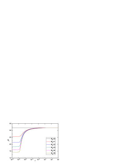
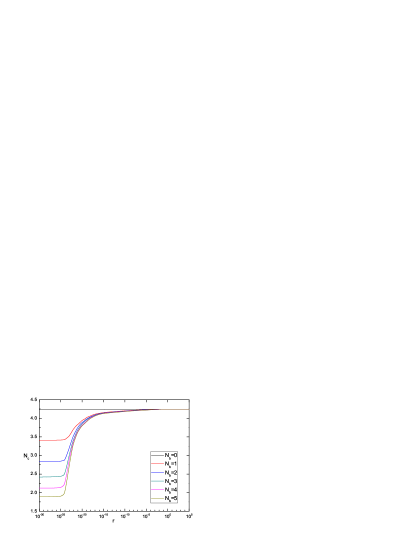
Figure 2: (a) Dependence of critical flavor $N_{f}^{c}$ on scalar boson mass $r$ for different values of boson flavor $N_{b}$ in the Landau gauge. (b) Dependence of critical flavor $N_{f}^{c}$ on scalar boson mass $r$ for different values of boson flavor $N_{b}$ in the non-local gauge.

When the scalar bosons condense, $\langle z_{\alpha}\rangle\neq 0$, the gauge boson becomes massive due to Anderson-Higgs mechanism. The effect of gauge boson mass on $N_{f}^{c}$ has been discussed previously in Ref. [22], where it was found that this mass rapidly suppresses the dynamical mass generation for Dirac fermions. We will not repeat such considerations in the present paper.

When applying the effective field theory to realistic cuprate superconductors, the Dirac fermions actually have two velocities, $v_{F}$ and $v_{\Delta}$, with $v_{F}/v_{\Delta}\approx 20$ [1]. Although the velocity anisotropy is important in certain physical quantities, it was shown [23] to be irrelevant near the critical point of chiral phase transition. Indeed, in most publications on spinor QED₃ the velocities are simply set to unity, i.e., $v_{F}=v_{\Delta}=1$ [1, 4, 5, 6, 9].

3 Classical potential of gauge field: confinement and deconfinement

The matter fields interact with each other through the mediation of U(1) gauge field. The classical potential between two particles with opposite gauge charges can be written in the coordinate space as [13]

$$V(\mathbf{x})=-\int\frac{d^{2}q}{(2\pi)^{2}}e^{i\mathbf{q}\cdot\mathbf{x}}\frac{1}{\mathbf{q}^{2}[1+\Pi(\mathbf{q}^{2})]}.$$ (21)

It has the following asymptotic form [13]

$$V(\mathbf{x})\sim\frac{1}{2\pi}\frac{1}{1+\Pi(0)}\ln(|\mathbf{x}|).$$ (22)

Obviously, the potential is determined by the infrared behavior of vacuum polarization function. In the absence of vacuum polarization $\Pi(q^{2})$, the potential has a logarithmical form

$$V(\mathbf{x})\sim\ln(|\mathbf{x}|).$$ (23)

This potential increases at large distances and hence is a confining potential, though weaker than a linear potential. When the polarization $\Pi(q^{2})$ is included, the gauge potential will be changed.

In cases without scalar field, $N_{b}=0$, the form of gauge potential $V(\mathbf{x})$ depends only on whether the fermion mass is zero or finite [14]. For massless fermion, the vacuum polarization is $\Pi(q^{2})=\frac{N_{f}}{8|q|}$. Since $\Pi(0)\rightarrow\infty$, the confining potential is destroyed. After the fermion mass is generated, the polarization function $\Pi_{a}^{f}(q^{2})$ becomes

$$\Pi_{a}^{f}(q^{2})=\frac{N_{f}}{4\pi q^{2}}\Big{(}2m+\frac{q^{2}-4m^{2}}{q}\arcsin\frac{q}{\sqrt{q^{2}+4m^{2}}}\Big{)}.$$

In the limit $q\rightarrow 0$, it has a finite value

$$\Pi_{a}^{f}(0)=\frac{N_{f}}{8\pi m}.$$ (24)

Thus in the symmetry breaking phase, the gauge potential is confining and there can not be any asymptotic fermion states [14].

Note the gauge field considered here is non-compact and there are no topological instanton configurations. The confinement is induced completely by the gauge force between particles with opposite charges. It is a special feature of gauge field in two spatial dimensions.

However, the gauge potential $V(\mathbf{x})$ is modified by the additional scalar boson. Depending on the fermion mass $m$ and the scalar boson mass $r$, there are four possibilities:

1. if $m=r=0$, $\Pi(q^{2})=\frac{2N_{f}+N_{b}}{16|q|}$ diverges at $q\rightarrow 0$;

2. if $m\neq 0$ and $r=0$, $\Pi(0)=\frac{N_{f}}{m}+\frac{N_{b}}{16|q|}$ diverges at $q\rightarrow 0$;

3. if $m=0$ and $r\neq 0$, $\Pi(0)=\frac{N_{f}}{8|q|}+\frac{N_{b}}{r}$ diverges at $q\rightarrow 0$;

4. if $m\neq 0$ and $r\neq 0$, $\Pi(0)=\frac{N_{f}}{m}+\frac{N_{b}}{r}$ is finite.

Compared with the case without scalar bosons, there appears a new possibility: at exactly the critical point where $r=0$, the gauge potential is always deconfined, irrespective of whether the chiral symmetry is broken or not. This implies that, in the chiral symmetry broken phase, the matter fields carrying internal gauge charges are deconfined at the quantum critical point $r=0$, but are always confined once the system enters the Coulomb phase with $r\neq 0$. The deconfined matter fields will make finite contribution to observable physical quantities, such as specific heat and susceptibility, but the confined matter fields make no contributions to them. In the confining phase, only excitations with zero gauge charge can be mobile and make finite contributions to observable quantities. Obviously, the quantum critical point and the Coulomb phase have rather different low-energy elementary excitations. It is possible to distinguish the critical point from the Coulomb phase by measuring the observable quantities. These quantities can also be used to judge whether dynamical chiral symmetry breaking happens or not.

4 Deconfinement and observable quantities at the quantum critical point $r=0$

We first discuss the quantum critical point, $r=0$, where the Dirac fermions and $z$ bosons are deconfined. In this point, the low-energy elementary excitations are: massive Dirac fermion $\psi$, massless scalar boson $z$, and composite massless Goldstone boson. The gauge field is strongly interacting with Dirac fermions and scalar bosons, so it makes finite contributions to the specific heat and susceptibility.

We first calculate the free energy $\mathcal{F}$ of the system, which is given by

$$\mathcal{F}=N_{b}f^{0b}+N_{f}f^{0f}+f^{G},$$ (25)

where $f^{0b}$, $f^{0f}$, and $f^{G}$ are the free energy of free scalar bosons, free fermions, and Goldstone bosons, respectively. To calculate the susceptibility, we follow the strategy of Ref. [9] and introduce two magnetic fields, $H_{b}$ and $H_{f}$. For $z$ bosons, the field shifts frequency as $\omega_{n}\rightarrow\omega_{n}-\theta H_{b}/2$, where $\theta=\pm 1$. For fermions, the coupling is the same, with the replacement $\omega_{n}\rightarrow\omega_{n}-\theta H_{f}$. Then the susceptibility $\chi$ and specific heat $C_{V}$ can be computed by

$$\chi_{b} = \frac{\partial^{2}\mathcal{F}}{\partial H_{b}^{2}},$$ (26)

$$\chi_{f} = \frac{\partial^{2}\mathcal{F}}{\partial H_{f}^{2}},$$ (27)

$$C_{V} = -T\frac{\partial^{2}\mathcal{F}}{\partial T^{2}}.$$ (28)

If the system is completely critical, the specific heat has the typical behavior $\sim T^{2}$. Once the Dirac fermion gets massive, the system is surely no longer critical and the $\sim T^{2}$ behavior must be changed. In order to make comparison, we still write the specific heat at low-$T$ in the form

$$C_{V}=\mathcal{A}_{C_{V}}T^{2},$$ (29)

where the coefficient

$$\mathcal{A}_{C_{V}}\!=\!N_{b}\mathcal{A}^{0b}_{C_{V}}+N_{f}\mathcal{A}^{0f}_{C_{V}}+\mathcal{A}^{G}_{C_{V}},$$ (30)

depends on temperature $T$. The susceptibility is linear in temperature $T$ when the system is critical, but also deviates from this behavior when the fermion becomes massive. It has the form

$$\chi_{b}=\mathcal{A}_{\chi_{b}}^{0b}T,$$ (31)

for scalar boson $z$ and

$$\chi_{f}=\mathcal{A}_{\chi_{f}}^{0f}T,$$ (32)

for fermion $\psi$. The susceptibility for Goldstone bosons certainly vanishes since they do not couple to any magnetic field.

4.1 $z$ scalar bosons

When the system is not at the critical point, $r\neq 0$, all matter fields carrying internal gauge charges are confined. Therefore, their contributions to specific heat $C_{V}^{0b}$ and susceptibility $\chi^{0b}$ strictly vanish at low-$T$. We only need to consider the point of $r=0$, where the free energy is given by

$$f^{0b}=\frac{T}{2}\sum_{\omega_{n}}\int\frac{d^{2}k}{4\pi^{2}}[\ln(k^{2}+(\omega_{n}+H_{b}/2)^{2}+m_{b}^{2})+\ln(k^{2}+(\omega_{n}-H_{b}/2)^{2}+m_{b}^{2})]-\frac{m_{b}^{2}}{g}.$$ (33)

The parameter $m_{b}$ depends on $T$ and field $H_{b}$ as [9]

$$\!m_{b}\!=\!T\!\ln\!\left\{\frac{2\cos(H_{b}/2T)+1+\sqrt{(2\cos(H_{b}/2T)+1)^{2}-4}}{2}\!\right\}.$$

The contributions of $z$ bosons to specific heat and susceptibility have been computed by Kaul and Sachdev [9], with the results

$$\mathcal{A}^{0b}_{C_{V}} = 6\frac{8\zeta(3)}{10\pi}\approx 1.83661,$$ (34)

$$\mathcal{A}_{\chi_{b}}^{0b} = \frac{\sqrt{5}}{4\pi}\ln\frac{\sqrt{5}+1}{2}\approx 0.0856271.$$ (35)

4.2 Massive fermions

At low but finite temperature $T$, the fermion mass should be a function $m(T,\mathbf{k})$ of $T$ and momenta $\mathbf{k}$. It is usually difficult to get an analytical expression of $m(T,\mathbf{k})$. As an approximation, we replace this function by a constant $m$, which might be identified by the value $m(0,0)$ at the limits $T=0,\mathbf{k}=0$. When $r=0$, the free energy of massive fermions is

$$f^{0f} = -T\int\frac{d^{2}k}{4\pi^{2}}[\ln(1+e^{-(\sqrt{k^{2}+m^{2}}+iH_{f})/T})+\ln(1+e^{-(\sqrt{k^{2}+m^{2}}-iH_{f})/T})],$$ (36)

from which the specific heat of massive fermions is found to be

$$\mathcal{A}^{0f}_{C_{V}} = \frac{1}{\pi}\Big{[}-(\frac{m}{T})^{3}\frac{e^{\frac{m}{T}}}{1+e^{\frac{m}{T}}}+3(\frac{m}{T})^{2}\ln[1+e^{\frac{m}{T}}]+6(\frac{m}{T})\textrm{Li}_{2}[-e^{\frac{m}{T}}]-6\textrm{Li}_{3}[-e^{\frac{m}{T}}]\Big{]}.$$ (37)

Here, $\textrm{Li}_{n}[z]$ is polylogarithm function.

At the limit $m\rightarrow 0$, it reduces to

$$-\frac{6}{\pi}\textrm{Li}_{3}[-1]=6\frac{3\zeta(3)}{4\pi}.$$ (38)

The dependence of $\mathcal{A}^{0f}_{C_{V}}$ on $\frac{m}{T}$ is depicted in Fig. 3. The susceptibility of massive fermions is

$$\mathcal{A}_{\chi_{f}}^{0f} = \frac{1}{\pi}\big{(}-\frac{\frac{m}{T}e^{\frac{m}{T}}}{1+e^{\frac{m}{T}}}+\ln[1+e^{\frac{m}{T}}]\big{)}.$$ (39)

As $m\rightarrow 0$, it approaches $\frac{\ln 2}{\pi}$. For finite $m$, the dependence of $\mathcal{A}^{0f}_{\chi_{f}}$ on $\frac{m}{T}$ is shown in Fig. 3. It is obvious that the mass suppresses the fermion contributions to both specific heat and susceptibility. Comparing with the contribution to specific heat from the $z$ bosons, the contribution of massive fermions can be simply neglected.

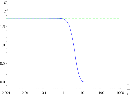
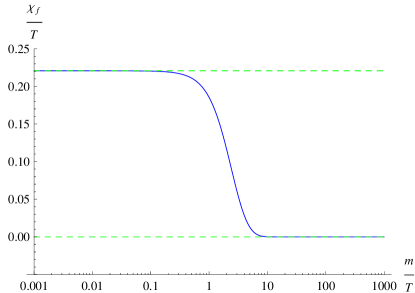
Figure 3: (a) Specific heat of massive fermions at very low $T$. The top dashed line corresponds to $\mathcal{A}^{0f}_{C_{V}}=\frac{9\zeta(3)}{2\pi}$. (b) Susceptibility of massive fermions at very low $T$. The top dashed line corresponds to $\mathcal{A}^{0f}_{\chi_{f}}=\frac{\ln 2}{\pi}$.

4.3 Goldstone bosons

Since the composite Goldstone bosons are neutral with respect to gauge charges, they are not confined by the gauge potential and can make finite contributions to certain observable quantities. At $r\neq 0$, the Goldstone bosons are the only degrees of freedom at very low-energy regime. Their contributions to specific heat are nonzero and have the same expression at both $r=0$ and $r\neq 0$. The free energy for Goldstone bosons is

$$f^{G}=T\sum_{\omega_{n}}\int\frac{d^{2}k}{4\pi^{2}}[\ln(k^{2}+\omega_{n}^{2})]=-\frac{2T^{3}\zeta(3)}{\pi}.$$ (40)

The specific heat is $\mathcal{A}^{G}_{C_{V}}T^{2}$ with

$$\mathcal{A}^{G}_{C_{V}}=-\frac{1}{T}\frac{\partial^{2}f^{G}}{\partial T^{2}}=12\frac{\zeta(3)}{\pi}\approx 4.591519.$$ (41)

Their contribution to susceptibility is zero because they do not couple to any magnetic field.

4.4 Gauge contributions to physical quantities at critical point $r=0$

At the deconfined critical point, $r=0$, the gauge field might give rise to important contributions to specific heat and susceptibility. The effective theory contains both temporal and spatial components of the gauge field, so there is no singular corrections to the free energy [4, 24].

To calculate the gauge field corrections to free energy, we should first obtain the polarization functions. The Feynman diagrams for the fermion and scalar boson contributions to polarization functions of gauge field are presented in Fig. 1. At finite temperature, the one-loop vacuum polarization tensor are defined as

$$\Pi_{\mu\nu}^{f}(p_{0},\mathbf{p}) = -\frac{N_{f}}{\beta}\sum_{n}\int\frac{d^{2}\mathbf{k}}{(2\pi)^{2}}\frac{\mathrm{Tr}[\gamma_{\mu}k\!\!\!/\gamma_{\nu}(p\!\!\!/+k\!\!\!/)]}{k^{2}(p+k)^{2}},$$

$$\Pi_{\mu\nu}^{b}(p_{0},\mathbf{p}) = -\frac{N_{b}}{\beta}\sum_{n}\int\frac{d^{2}\mathbf{k}}{(2\pi)^{2}}\left[\frac{(p+2k)_{\mu}(p+2k)_{\nu}}{k^{2}(p+k)^{2}}-\frac{\delta_{\mu\nu}}{k^{2}}\right].$$ (42)

Here, the Matsubara frequency is $p_{0}=2m\pi/\beta$ for gauge boson, $k_{0}=2n\pi/\beta$ for scalar boson, and the frequency is $k_{0}=(2n+1)\pi/\beta$ for Dirac fermion. Using the transverse condition, $p^{\mu}\Pi_{\mu\nu}=0$, the polarization tensor can be decomposed as

$$\Pi_{\mu\nu}(p_{0},\mathbf{p}) = [\Pi_{A}^{f}(p_{0},\mathbf{p})+\Pi_{A}^{b}(p_{0},\mathbf{p})]A_{\mu\nu}+[\Pi_{B}^{f}(p_{0},\mathbf{p})+\Pi_{B}^{b}(p_{0},\mathbf{p})]B_{\mu\nu},$$ (43)

where

$$A_{\mu\nu} = \left(\delta_{\mu 0}-\frac{p_{\mu}p_{0}}{p^{2}}\right)\frac{p^{2}}{\mathbf{p}^{2}}\left(\delta_{0\nu}-\frac{p_{0}p_{\nu}}{p^{2}}\right),$$

$$B_{\mu\nu} = \delta_{\mu i}\left(\delta_{ij}-\frac{p_{i}p_{j}}{\mathbf{p}^{2}}\right)\delta_{j\nu},$$ (44)

which satisfy the relationship

$$A_{\mu\nu}+B_{\mu\nu}=\delta_{\mu\nu}-\frac{p_{\mu}p_{\nu}}{p^{2}}.$$ (45)

Now the gauge boson propagator can be written as

$$D_{\mu\nu}(p_{0},\mathbf{p}) = \frac{A_{\mu\nu}}{p^{2}+\Pi_{A}^{f}(p_{0},\mathbf{p})+\Pi_{A}^{b}(p_{0},\mathbf{p})}+\frac{B_{\mu\nu}}{p^{2}+\Pi_{B}^{f}(p_{0},\mathbf{p})+\Pi_{B}^{b}(p_{0},\mathbf{p})}.$$ (46)

The gauge contribution to free energy is given by:

$$f^{1A}(\beta,H_{f})=\frac{T}{2}\sum_{\epsilon_{m}}\int\frac{d^{2}k}{(2\pi)^{2}}\ln\Big{[}(p^{2}+\Pi_{A}^{f}+\Pi_{A}^{b})(p^{2}+\Pi_{B}^{f}+\Pi_{B}^{b})\Big{]}.$$ (47)

The vacuum functions $\Pi_{A}^{f}$, $\Pi_{A}^{b}$, $\Pi_{B}^{f}$, and $\Pi_{B}^{b}$ should be calculated explicitly. They are related to the temporal and spatial components of vacuum polarization tensor $\Pi_{\mu\nu}^{f}$ and $\Pi_{\mu\nu}^{b}$ by the identities

$$\Pi_{A}^{f(b)} = \frac{p^{2}}{\mathbf{p}^{2}}\Pi_{00}^{f(b)},$$ (48)

$$\Pi_{B}^{f(b)} = \Pi_{ii}^{f(b)}-\frac{p_{0}^{2}}{\mathbf{p}^{2}}\Pi_{00}^{f(b)}.$$ (49)

In Ref. [9], the temporal and spatial components of polarization functions were obtained approximately. Indeed, these functions can be computed exactly even in the presence of finite magnetic field $H_{f,b}$ and fermion mass $m$. Using the methods presented in Ref. [25], we obtained the following expressions for the fermion contribution to polarization functions

$$\Pi_{00}^{f}(\epsilon_{m},\mathbf{k}) = \frac{N_{f}}{\pi\beta}\int_{0}^{1}dx\ln[4D_{m}(x,\epsilon_{m},\mathbf{k},H_{f})]-\frac{N_{f}}{4\pi}\int_{0}^{1}dx(1-2x)\epsilon_{m}\frac{\sin(x\beta\epsilon_{m}-\beta\theta H_{f})}{D_{m}(x,\epsilon_{m},\mathbf{k},H_{f})}$$

$$-\frac{N_{f}}{2\pi}\int_{0}^{1}dx\frac{m^{2}+x(1-x)\epsilon_{m}^{2}}{E_{f}D_{m}(x,\epsilon_{m},\mathbf{k},H_{f})}\sinh(\beta E_{f}),$$

$$\Pi_{11}^{f}(\epsilon_{m},\mathbf{k})=\Pi_{22}^{f}(\epsilon_{m},\mathbf{k})$$

$$= -\frac{N_{f}}{4\pi}\int_{0}^{1}dx\frac{(1-2x)\epsilon_{m}\sin(x\beta\epsilon_{m}-\beta\theta H_{f})}{D_{m}(x,\epsilon_{m},\mathbf{k},H_{f})}-\frac{N_{f}}{4\pi}\int_{0}^{1}dx\frac{x(1-x)(\mathbf{k}^{2}+2\epsilon_{m}^{2})}{E_{f}D_{m}(x,\epsilon_{m},\mathbf{k},H_{f})}\sinh(\beta E_{f}).$$

The corresponding expressions for scalar bosons are

$$\Pi_{00}^{b}(\epsilon_{m},\mathbf{k}) = \frac{N_{b}}{2\pi\beta}\int_{0}^{1}dx\ln\left[4J_{m}(x,\epsilon_{m},\mathbf{k},H_{b})\right]-\frac{N_{b}}{4\pi}\int_{0}^{1}dx(1-x)\epsilon_{m}\frac{\sin(x\beta\epsilon_{m}-\frac{\beta}{2}\theta H_{b})}{J_{m}(x,\epsilon_{m},\mathbf{k},H_{b})}$$

$$-\frac{N_{b}}{4\pi}\int_{0}^{1}dx\frac{\frac{1}{2}x\mathbf{k}^{2}-(x^{2}-\frac{3}{2}x+\frac{1}{4})\epsilon_{m}^{2}}{E_{b}J_{m}(x,\epsilon_{m},\mathbf{k},H_{b})}\sinh(\beta E_{b}),$$

$$\Pi_{11}^{b}(\epsilon_{m},\mathbf{k})=\Pi_{22}^{b}(\epsilon_{m},\mathbf{k})$$

$$= -\frac{N_{b}}{4\pi}\int_{0}^{1}dx\frac{x\epsilon_{m}\sin(x\beta\epsilon_{m}-\frac{\beta}{2}\theta H_{b})}{J_{m}(x,\epsilon_{m},\mathbf{k},H_{b})}+\frac{N_{b}}{8\pi}\int_{0}^{1}dx\frac{x(1-x)(\mathbf{k}^{2}+\epsilon_{m}^{2})+\frac{1}{2}k_{1}^{2}-x^{2}\epsilon_{m}^{2}}{E_{b}J_{m}(x,\epsilon_{m},\mathbf{k},H_{b})}\sinh(\beta E_{b}).$$

Here, we have defined a list of functions:

$$D_{m}(x,\epsilon_{m},\mathbf{k},H_{f}) = \cosh^{2}(\frac{1}{2}\beta E_{f})-\sin^{2}(\frac{1}{2}x\beta\epsilon_{m}-\frac{\beta}{2}\theta H_{f}),$$

$$E_{f}(x,\epsilon_{m},\mathbf{k},m) = \sqrt{m^{2}+x(1-x)(k^{2}+\epsilon_{m}^{2})},$$

$$J_{m}(x,\epsilon_{m},\mathbf{k},H_{b}) = \cosh^{2}(\frac{1}{2}\beta E_{b})-\sin^{2}(\frac{1}{2}x\beta\epsilon_{m}-\frac{\beta}{4}\theta H_{b}),$$

$$E_{b}(x,\epsilon_{m},\mathbf{k}) = \sqrt{x(1-x)(k^{2}+\epsilon_{m}^{2})}.$$

Note the scalar mass is taken to be $r=0$ since the gauge field is deconfined only at this critical point.

The field $\lambda$ has dynamics only by integrating out the boson fields $z$, which leads to the following free energy

$$f^{1\lambda}(\beta,H_{b}) = \frac{1}{2\beta}\sum_{\epsilon_{m}}\int\frac{d^{2}k}{(2\pi)^{2}}\ln\left[\Pi_{\lambda}(\epsilon_{m},\mathbf{k})\right],$$ (50)

where the vacuum polarization, given by Fig. 1, at finite temperature is

$$\Pi_{\lambda}(\epsilon_{m},\mathbf{k})=\frac{N_{b}}{16\pi}\int_{0}^{1}dx\frac{1}{E_{b}}\frac{\sinh(\beta E_{b})}{J_{m}(x,\epsilon_{m},\mathbf{k},H_{b})}.$$ (51)

Now we are ready to calculate the gauge field corrections to free energy $f^{1A}$ and $f^{1\lambda}$ by inserting the polarization functions $\Pi_{A}^{f}$, $\Pi_{A}^{b}$, $\Pi_{B}^{f}$, $\Pi_{B}^{b}$ into (47) and $\Pi_{\lambda}$ into (50). Then the specific heat and susceptibility can be obtained by taking derivatives of the free energy with respect to $T$ and $H_{f,b}$, respectively. After numerical computations, the results for specific heat and susceptibility are presented in Fig. 4 and Fig. 5. Apparently, the gauge contributions to specific heat and susceptibility are significantly suppressed by the mass of Dirac fermions. Here, in order to show the explicit results, we use the absolute value of $|\mathcal{A}^{1\lambda}_{C_{V}}|=-\mathcal{A}^{1\lambda}_{C_{V}}$ ($|\mathcal{A}^{1\lambda}_{\chi_{b}}|=-\mathcal{A}^{1\lambda}_{\chi_{b}}$) instead of $\mathcal{A}^{1\lambda}_{C_{V}}$ ($\mathcal{A}^{1\lambda}_{\chi_{b}}$). Although $r=0$ at the critical point, for completeness we also present the results for some magnitudes of finite $r$ in Fig. 5. If $N_{f}>N_{f}^{c}$, the fermions remain massless and the matter fields carrying internal gauge charges are not confined at finite $r$. In such state, the mass $r$ suppresses the specific heat and susceptibility of $z$ bosons.

In summary, at the critical point $r=0$, both fermionc and gauge field contributions to specific heat and susceptibility are suppressed by the dynamical fermion mass. At low temperature, the total specific heat receives contributions mainly from three parts: free scalar boson $z$, the composite Goldstone boson, and the fluctuation of field $\lambda$. Since the $z$ and Goldstone bosons are both massless, these three contributions to specific heat are all proportional to $T^{2}$, with coefficients $\mathcal{A}_{C_{V}}$ being temperature independent. However, the scalar bosons carry nonzero internal gauge charge, while the Goldstone bosons are neutral. Therefore, the former lead to a $\propto T$ susceptibility (to $H_{b}$), while the latter does not couple to any magnetic field ($H_{f}$, $H_{b}$, or the physical $H$) and hence make no contribution to susceptibility.

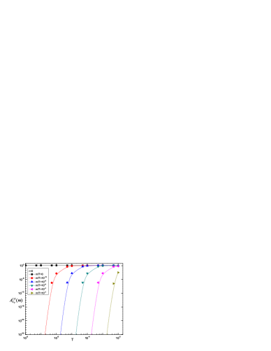
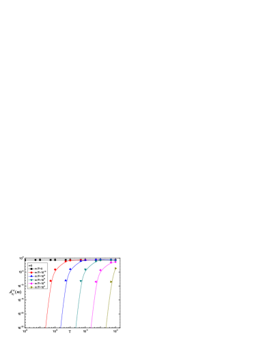
Figure 4: (a) The gauge field contribution to specific heat for different fermion mass. (b) The gauge field contribution to susceptibility for different fermion mass.

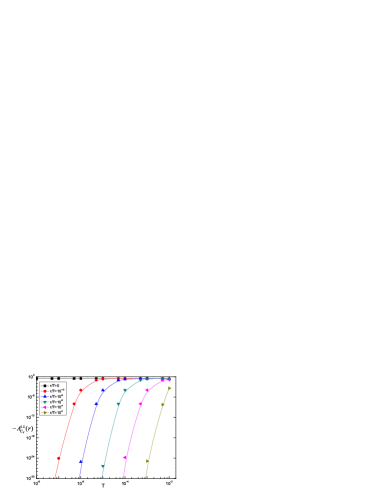
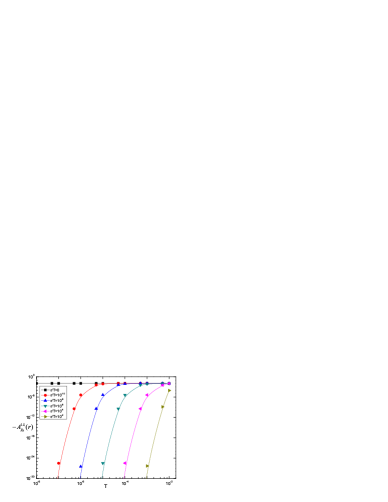
Figure 5: (a) The contribution of field $\lambda$ to specific heat for different boson mass. (b) The contribution of field $\lambda$ to susceptibility for different boson mass.

5 Confinement and observable quantities at $r\neq 0$

We now consider the Coulomb phase with $r\neq 0$. Once the logarithmic gauge potential confines all particles that carry internal gauge charges, the excitations appearing at low energy regime must be neutral with respect to internal gauge charge. Now the massive fermions can combine either with anti-fermions or with massive scalar bosons carrying opposite gauge charges. In the former case, the corresponding composite particles are just the massless Goldstone bosons. In the later case, the separated spin and electric charge degrees of freedom are re-combined by the confining internal gauge potential. This implies that there are also electron-like quasiparticles that carry both $1/2$-spin and $-e$ electric charge. It is a nontrivial task to estimate their mass since this requires a clear understanding about the mechanism of spin-charge recombination. The issue of spin-charge recombination has been investigated for many years by several authors [5, 6, 26, 27]. Unfortunately, this issue is not at all clear. In the absence of a reliable theory for spin-charge recombination, here we assume a constant mass $m_{e}$. Further, the $z$ bosons can combine with the $z^{\ast}$ bosons to form composite spin excitations [7, 8, 9]. Both the electron-like fermionic quasiparticles and the composite spin excitations are gapped, so their contributions to specific heat and susceptibility (with respect to real magnetic field $H$, rather than $H_{f,b}$) are suppressed by their mass gaps $m_{e}$ and $\Delta_{\mathrm{spin}}$. At very low temperatures, only the composite Goldstone bosons contribute to specific heat (see equation (41)). However, although having the same $T$-dependence at the point $r=0$, the magnitude of specific heat in the Coulomb phase is much smaller than that at $r=0$ since the contributions from massless $z$ bosons and the field $\lambda$ all disappear at $r\neq 0$ due to confinement.

6 Summary and discussion

In summary, we have studied the possible mass generation of initially massless Dirac fermions in a continuum U(1) gauge field theory in (2+1) dimensions. It was found that a dynamical mass is generated when the fermion flavor $N_{f}$ is less than $N_{f}^{c}$ which has quantitatively different values at the quantum critical point $r=0$ and at $r\neq 0$. The gauge potential between charged particles leads to logarithmic confinement when $r\neq 0$, but at the critical point $r=0$ the matter fields carrying nonzero internal gauge charge are deconfined. The low-energy properties of the system at $r=0$ are quite different from those at $r\neq 0$. We discussed some observable physical quantities, including specific heat and susceptibility, of the system at low temperature and argued that they can be used to judge whether the system stays at the quantum critical point $r=0$ and whether the fermions acquire a dynamical mass.

Besides specific heat and susceptibility, the happening of dynamical fermion gap generation can also be readily seen from the transport properties of the system. At very low temperature, the thermal conductivity is mainly determined by the low-lying fermionic excitations. If the Dirac fermions are massless, then they exhibit universal thermal conductivity, $\frac{\kappa}{T}=\frac{1}{3}\frac{v_{F}^{2}+v_{\Delta}^{2}}{v_{F}v_{\Delta}}$, which is independent of impurity scattering rate $\Gamma_{0}$ [28]. Once the Dirac fermions acquire a dynamical mass $m$, then the thermal conductivity at zero temperature becomes $\frac{\kappa}{T}=\frac{1}{3}\frac{v_{F}^{2}+v_{\Delta}^{2}}{v_{F}v_{\Delta}}\frac{\Gamma_{0}^{2}}{\Gamma_{0}^{2}+m^{2}}$, which is no longer universal and is reduced by the fermion mass [29]. If the system is in the clean limit so that $\Gamma_{0}\ll m$, then the thermal conductivity vanishes at very low temperature.

When chiral symmetry is dynamically broken (no matter $r=0$ or $r\neq 0$), there are no gapless fermionic excitations at low temperature. Therefore, in the limit $\Gamma_{0}\ll m$ the thermal conductivity effectively vanishes at zero temperature and does not have a universal linear term that would exist if the system contains gapless Dirac fermions. The ground state of the system corresponds to an interesting state of matter where the specific heat exhibits behavior of gapless (bosonic) excitations but the thermal conductivity has no residual linear term. In two recent works, thermodynamic measurements carried out in $\kappa$-(BEDT-TTF)₂Cu₂(CN)₃ found evidence for the presence of gapless excitations [30], while thermal transport measurements carried out in the same material found good evidence supporting the absence of gapless fermionic excitations [31]. Although it is not known whether the ground state of $\kappa$-(BEDT-TTF)₂Cu₂(CN)₃ can be described by a continuum field theory analogous to the combined action $\mathcal{S}_{f}+\mathcal{S}_{b}$, such seemingly contradicting experimental facts are consistently realized by the chiral symmetry breaking phase of action $\mathcal{S}_{f}+\mathcal{S}_{b}$ and can be naturally understood by the mechanism discussed in the context.

The analysis presented above can also be applied to the Abelian Higgs model, which may be considered as the relativistic version of Ginzburg-Landau model, with Higgs field being the superconducting order parameter. Although the $CP^{N_{b}-1}$ model is distinct in physical contents from the Abelian Higgs model, its low-energy property bears much resemblance to that of the latter.

References

- [1] P.A. Lee, N. Nagaosa, X.-G. Wen, Rev. Mod. Phys. 78 (2006) 17.
- [2] I. Affleck, J.B. Marston, Phys. Rev. B 37 (1988) 3774.
- [3] L. B. Ioffe, A.I. Larkin, Phys. Rev. B 39 (1989) 8988.
- [4] D.H. Kim, P.A. Lee, X.-G. Wen, Phys. Rev. Lett. 79 (1997) 2109.
- [5] D.H. Kim, P.A. Lee, Ann. Phys. (N.Y.) 272 (1999) 130.
- [6] W. Rantner, X.-G. Wen, Phys. Rev. Lett. 86 (2001) 3871.
- [7] T. Senthil, A. Vishwanath, L. Balents, S. Sachdev, M.P.A. Fisher, Science 303 (2004) 1490; T. Senthil, L. Balents, S. Sachdev, A. Vishwanath, M.P.A. Fisher, Phys. Rev. B 70 (2004) 144407.
- [8] R.K. Kaul, A. Kolezhuk, M. Levin, S. Sachdev, S. Senthil, Phys. Rev. B 75 (2007) 235122; R. K. Kaul, Y.B. Kim, S. Sachdev, S. Senthil, Nature Physics 4 (2008) 28.
- [9] R.K. Kaul, S. Sachdev, Phys. Rev. B 77 (2008) 155105.
- [10] T. Appelquist, D. Nash, L.C.R. Wijewardhana, Phys. Rev. Lett. 60 (1988) 2575.
- [11] D. Nash, Phys. Rev. Lett. 62 (1989) 3024.
- [12] E. Dagotto, J.B. Kogut, A. Kocić, Phys. Rev. Lett. 62 (1989) 1083.
- [13] C.J. Burden, J. Praschifka, C.D. Roberts, Phys. Rev. D 46 (1992) 2695.
- [14] P. Maris, Phys. Rev. D 52 (1995) 6087.
- [15] M. Hermele, T. Senthil, M.P.A. Fisher, P.A. Lee, N. Nagaosa, X.-G. Wen, Phys. Rev. B 70 (2004) 214437.
- [16] S. Takashima, I. Ichinose, T. Matsui, Phys. Rev. B 73 (2006) 075119.
- [17] Renormalization group analysis showed that the critical fermion flavor beyond which deconfinement occurs is as large as . See, F.S. Nogueira, H. Kleinert, Phys. Rev. B 77 (2008) 045107.
- [18] Y. Nambu, G. Jona-Lasinio, Phys. Rev. 122 (1961) 345.
- [19] A.M. Polyakov, Gauge Fields and Strings (Harwood, Academic, Chur, Switzerland, 1987).
- [20] L.D. Landau, I.M. Khalatnikov, JETP 2 (1956) 69; B. Zumino, J. Math. Phys. 1 (1960) 1.
- [21] H. Georgi, E.H. Simmons, A.G. Cohen, Phys. Lett. B 236 (1990) 183; T. Kugo, M.G. Mitchard, Phys. Lett. B 282 (1992) 162; T. Ebihara, T. Iizuka, K.-I. Kondo, E. Tanaka, Nucl. Phys. B 434 (1995) 8; K.-I. Kondo, Phys. Rev. D 55 (1997) 7826.
- [22] G.-Z. Liu and G. Cheng, Phys. Rev. D 67 (2003) 065010; H. Jiang, G.-Z. Liu, G. Cheng, J. Phys. A 41 (2008) 255402.
- [23] D.J. Lee, I.F. Herbut, Phys. Rev. B 66 (2002) 094512; O. Vafek, Z. Tesanovic, M. Franz, Phys. Rev. Lett. 89 (2002) 157003.
- [24] Y. Ran, M. Hermele, P.A. Lee, X.-G. Wen, Phys. Rev. Lett. 98 (2007) 117205.
- [25] W. Li, G.-Z. Liu, arXiv: 0907.2365v1.
- [26] C. Mudry, E. Fradkin, Phys. Rev. B 49 (1994) 5200.
- [27] G.-Z. Liu, Phys. Rev. B 71 (2005) 172501.
- [28] A. Durst, P. A. Lee, Phys. Rev. B 62 (2000) 1270.
- [29] V. P. Gusynin and V. A. Miransky, Eur. Phys. J. B 37 (2003) 363.
- [30] S. Yamashita, Y. Nakazawa, M. Oguni, Y. Oshima, H. Nojiri, Y. Shimizu, K. Miyagawa, K. Kanoda, Nature Phys. 4 (2008) 459.
- [31] M. Yamashita, N. Nakata, Y. Kasahara, T. Sasaki, N. Toneyama, N. Kobayashi, S. Fujimoto, T. Shibauchi, Y. Matsuda, Nature Phys. 5 (2008) 44.