Quantum teleportation scheme by selecting one of multiple output ports

Abstract

The scheme of quantum teleportation, where Bob has multiple ($N$) output ports and obtains the teleported state by simply selecting one of the $N$ ports, is thoroughly studied. We consider both deterministic version and probabilistic version of the teleportation scheme aiming to teleport an unknown state of a qubit. Moreover, we consider two cases for each version: (i) the state employed for the teleportation is fixed to a maximally entangled state, and (ii) the state is also optimized as well as Alice’s measurement. We analytically determine the optimal protocols for all the four cases, and show the corresponding optimal fidelity or optimal success probability. All these protocols can achieve the perfect teleportation in the asymptotic limit of $N\rightarrow\infty$. The entanglement properties of the teleportation scheme are also discussed.

I Introduction

Quantum teleportation Bennett95b ; Boschi98a ; Bouwmeester97a ; Furusawa98a is a fundamental and important protocol for quantum information science and technology, by which an unknown quantum state is transfered from a sender (Alice) to a receiver (Bob) exploiting their prior shared entangled state (and with the assistance of classical communication). In the original (or standard) teleportation scheme for transferring a state of a qubit (quantum bit) Bennett95b , Alice first performs the Bell-state measurement on the state $|\chi_{\rm in}\rangle$ to be teleported and her half of a maximally entangled state $|\psi^{-}\rangle_{AB}=(|01\rangle-|10\rangle)/\sqrt{2}$. She then tells the outcome $k$ to Bob via a classical communication channel. To complete the teleportation, Bob applies a unitary transformation $\sigma_{k}$ to his half of $|\psi^{-}\rangle_{AB}$, where $\sigma_{0}\equiv\openone$ and $(\sigma_{1},\sigma_{2},\sigma_{3})$ are the Pauli matrices. Note that continuous-variable teleportation schemes have also been proposed and intensively studied Furusawa98a ; ContinuousVariable , where an entangled state on an infinite dimensional Hilbert space is employed. In this paper, however, we exclusively consider the schemes with discrete (spin) variables in a finite dimensional Hilbert space (though we also consider the limit of infinite dimension).

The quantum teleportation offers a more powerful function than simply transferring an unknown state Nielsen97a ; Gottesman99a . Consider that the state $|\varepsilon\rangle=(\openone\otimes\varepsilon)|\psi^{-}\rangle_{AB}$, instead of $|\psi^{-}\rangle_{AB}$, is employed for the standard teleportation scheme, where $\varepsilon$ is an arbitrary quantum operation. Bob then obtains $\sigma_{k}\varepsilon(\sigma_{k}|\chi_{\rm in}\rangle)$ as an output of the teleportation procedure, and thus, obtains $\varepsilon(|\chi_{\rm in}\rangle)$ when the outcome of the Bell-state measurement is $k=0$. This implies that the operations of the Bell-state measurement and the post-selection of the event with $k=0$ (these operations are denoted by $G$ as a whole) can perform the processing of $|\chi_{\rm in}\rangle\rightarrow\varepsilon(|\chi_{\rm in}\rangle)$ such that $G(|\chi_{\rm in}\rangle\otimes|\varepsilon\rangle)=\varepsilon(|\chi_{\rm in}\rangle)\otimes|\varepsilon^{\prime}\rangle$. The point is that $G$ depends on neither $\varepsilon$ nor $|\chi_{\rm in}\rangle$, but the fixed $G$ can perform the manipulation by $\varepsilon$ if an appropriate $|\varepsilon\rangle$ is provided. The device to manipulate a state in such a way is called a programmable quantum processor (in short, processor) Nielsen97a ; Gottesman99a ; Kim01a ; Vidal02c ; Fiurasek02a ; Fiurasek04a ; Brazier05a ; Ziman05a ; DAriano05a ; Hillery06a ; Garcia06a , because the function of the processor is programmed via $|\varepsilon\rangle$. Moreover, if a processor can be programmed to perform an arbitrary $\varepsilon$, it is called a universal processor. The standard teleportation scheme thus offers the function as a universal processor Nielsen97a , because $|\varepsilon\rangle$ is defined for an arbitrary $\varepsilon$ as $|\varepsilon\rangle=(\openone\otimes\varepsilon)|\psi^{-}\rangle_{AB}$. Note that, since the form of $|\varepsilon\rangle$ is known for given $\varepsilon$, we can generate it by various methods, and therefore an arbitrary state-manipulation can be replaced with a state-preparation as in Refs. Gottesman99a ; Knill01a . Note further that, even if $|\varepsilon\rangle$ is generated by applying $\varepsilon$ to $|\psi^{-}\rangle_{AB}$, we can receive a considerable benefit such that we can perform $\varepsilon$ before getting an input state $|\chi_{\rm in}\rangle$, i.e., the time-ordering of these two events can be exchanged private ; Brukner03a ; Imoto04a .

Unfortunately, however, the universal processor based on the standard teleportation scheme only works in a probabilistical way. This is because Bob’s unitary transformation $\sigma_{k}$ with $k\neq 0$ generally does not commute with $\varepsilon$, and hence $\sigma_{k}\varepsilon(\sigma_{k}|\chi_{\rm in}\rangle)\neq\varepsilon(|\chi_{\rm in}\rangle)$ in general for $k\neq 0$. As a result, the success probability of the universal processor is $1/4$.

On the other hand, in the teleportation scheme proposed by Knill, Laflamme, and Milburn (KLM) Knill01a ; Franson02a ; Grudka08a ; Modlawska08a ; Kok07a , Bob has multiple ($N$) output ports and obtains the teleported state by selecting one of the $N$ ports according to the outcome of Alice’s measurement. To complete the teleportation, Bob further needs to apply a unitary transformation (phase shift) to the state of the selected port, as well as the standard teleportation scheme. As shown in Ref. Ishizaka08b , however, the teleportation scheme such that Bob simply selects one of the $N$ ports (without any additional unitary transformation) is also possible (Fig. 1). In fact, the faithful and deterministic teleportation is asymptotically achieved in the limit of $N\rightarrow\infty$ Ishizaka08b . Let $|\psi\rangle$ be an entangled state employed for this teleportation scheme (see Fig. 1), and $\varepsilon^{\otimes N}$ denote the operation of applying $\varepsilon$ to every output port. Since the operation of simply selecting a port always commutes with $\varepsilon^{\otimes N}$, if the state $|\varepsilon\rangle=(\openone\otimes\varepsilon^{\otimes N})|\psi\rangle$ is employed for the teleportation, Bob obtains $\varepsilon(|\chi_{\rm in}\rangle)$ as an output of the teleportation procedure, regardless of which port is selected. In this way, this teleportation scheme can provide a faithful and deterministic universal processor in the asymptotic limit of $N\rightarrow\infty$ Ishizaka08b . Note, however, that such a teleportation scheme must be an approximate and/or probabilistic one if $N$ is finite, which is a consequence of the no-go theorem of a faithful and deterministic universal processor with finite system size Nielsen97a .

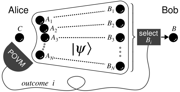
Figure 1: The setting of the teleportation scheme considered in this paper. Bob has multiple output ports and obtains the teleported state by simply selecting one of the $N$ ports according to the outcome ($i$) of Alice’s measurement. To complete the teleportation, no unitary transformation to each output port is necessary because the state of one of the $N$ ports becomes the teleported state as it is.

In this paper, the scheme of quantum teleportation, where Bob simply selects one of the $N$ ports, is thoroughly studied. We consider both deterministic version and probabilistic version of the teleportation scheme, and analytically determine the optimal protocols. The corresponding optimal fidelity or optimal success probability are shown as a function of $N$. This paper is organized as follows: The deterministic (and hence approximate) version of our teleportation scheme is formulated in Sec. II. The operator $\rho$ defined there [Eq. (6)] plays an important role for determining the optimal protocols, and hence the characteristics of $\rho$ is investigated and summarized in Sec. III. In Sec. IV, we determine the optimal protocols of the deterministic version, where we consider two cases: (i) the state $|\psi\rangle$ employed for the teleportation is fixed to a maximally entangled state, and (ii) the state $|\psi\rangle$ is also optimized as well as Alice’s measurement. The probabilistic version is then formulated in Sec. V, and the optimal protocols are determined in Sec. VI, where we again consider two cases (i) and (ii) as in Sec. IV. The simplest example of the probabilistic scheme with $N=2$ is explicitly shown in Sec. VII. Moreover, the entanglement properties are discussed in Sec. VIII. In particular, we focus on the amount of entanglement consumed during the teleportation procedure. Finally, a summary is given in Sec. IX.

II Deterministic version

In the deterministic version of our teleportation scheme, Bob always accepts the state of one of the $N$ ports as the teleported state, i.e., the teleportation is regarded to succeed with unit probability. As mentioned in the introduction, the deterministic teleportation scheme is necessarily an approximate one if $N$ is finite. The optimal protocol is then such that it maximizes the teleportation fidelity $f$ averaged over all uniformly distributed input pure states. Since the average fidelity is given by $f=(2F+1)/3$ Horodecki99a , the optimal protocol also maximizes the entanglement fidelity $F$.

Consider that Bob has $N$ qubits: $B_{1}$, $B_{2}$, $\cdots$, $B_{N}$, where each corresponds to the output port of the teleportation. Alice also has $N$ qubits: $A_{1}$, $A_{2}$, $\cdots$, $A_{N}$, which are denoted by $A$ as a whole. The state $|\psi\rangle$ on these $2N$ qubits is employed for teleporting an unknown state of the $C$ qubit (see Fig. 1). Note that the entanglement fidelity $F$ is maximized when the state employed for the teleportation is a pure state because of the convexity of $F$. Without loss of generality, $|\psi\rangle$ can be written as

$$|\psi\rangle=(O_{A}\otimes\openone_{B_{1}\cdots B_{N}})|\psi^{-}\rangle_{A_{1}B_{1}}|\psi^{-}\rangle_{A_{2}B_{2}}\cdots|\psi^{-}\rangle_{A_{N}B_{N}},$$

where $|\psi^{-}\rangle=(|01\rangle-|10\rangle)/\sqrt{2}$ is a maximally entangled state (spin-singlet state) and $O$ is an arbitrary operator that satisfies $\hbox{tr}O^{\dagger}O=2^{N}$ so that $|\psi\rangle$ is normalized.

Alice then performs a joint measurement with $N$ possible outcomes ($1$, $2$, $\cdots$, $N$) on the $A$ and $C$ qubits. The measurement is described by a positive operator valued measure (POVM) whose elements are $\{\Pi_{i}\}$ such that $\sum_{i=1}^{N}\Pi_{i}=\openone_{AC}$. Suppose that she obtains the outcome $i$. She then tells the outcome to Bob via a classical communication channel, and he discards the $(N-1)$ qubits of $B_{1}B_{2}\cdots B_{i-1}B_{i+1}\cdots B_{N}$, which are briefly denoted by ${\bar{B}}_{i}$. The state of the remaining $B_{i}$ qubit, which is regarded as the $B$ qubit, is the teleported state.

The corresponding teleportation channel, which maps the density matrices acting on the Hilbert space ${\cal H}_{C}$ to those on ${\cal H}_{B}$, is thus

$$\Lambda(\sigma^{\rm in}) =\sum_{i=1}^{N}\left[\hbox{tr}_{A{\bar{B}_{i}}C}\sqrt{\Pi_{i}}(|\psi\rangle\langle\psi|\otimes\sigma^{\rm in}_{C})\sqrt{\Pi_{i}}^{\dagger}\right]_{B_{i}\rightarrow B}$$

$$=\sum_{i=1}^{N}\hbox{tr}_{AC}\Pi_{i}\left([(O\otimes\openone)\sigma^{(i)}_{AB}(O^{\dagger}\otimes\openone)]\otimes\sigma^{\rm in}_{C}\right)$$ (1)

with

$$\sigma^{(i)}_{AB} =\left[\hbox{tr}_{\bar{B}_{i}}(P^{-}_{A_{1}B_{1}}\otimes P^{-}_{A_{2}B_{2}}\otimes\cdots\otimes P^{-}_{A_{N}B_{N}})\right]_{B_{i}\rightarrow B}$$

$$=\frac{1}{2^{N-1}}P^{-}_{A_{i}B}\otimes\openone_{\bar{A}_{i}},$$ (2)

where $P^{-}=|\psi^{-}\rangle\langle\psi^{-}|$, and ${\bar{A}}_{i}$ is a shorthand notation for $A_{1}A_{2}\cdots A_{i-1}A_{i+1}\cdots A_{N}$. The entanglement fidelity $F$ for the above channel $\Lambda$ is then given by

$$F =\hbox{tr}P^{-}_{BD}\left[(\Lambda\otimes\openone)P^{-}_{CD}\right]$$

$$=\hbox{tr}\sum_{i=1}^{N}P^{-}_{BD}\Pi_{iAC}\left([(O\otimes\openone)\sigma^{(i)}_{AB}(O^{\dagger}\otimes\openone)]\otimes P^{-}_{CD}\right)$$

$$=\frac{1}{2^{2}}\sum_{i=1}^{N}\hbox{tr}\Pi_{iAB}[(O\otimes\openone)\sigma^{(i)}_{AB}(O^{\dagger}\otimes\openone)]$$

$$=\frac{1}{2^{2}}\sum_{i=1}^{N}\hbox{tr}\tilde{\Pi}_{iAB}\sigma^{(i)}_{AB}.$$ (3)

Note that $\Pi_{i}$ is changed into an operator acting on ${\cal H}_{A}\otimes{\cal H}_{B}$ in the third equality of Eq. (3) because we used the relationship that $(V\otimes\openone)|\psi^{-}\rangle=(\openone\otimes\sigma_{2}V^{T}\sigma_{2})|\psi^{-}\rangle$ for any operator $V$, where $\sigma_{2}$ is the $y$-component of the Pauli matrices. Moreover, we introduced $\tilde{\Pi}_{i}=(O^{\dagger}\otimes\openone)\Pi_{i}(O\otimes\openone)$ in the last equality of Eq. (3), which must satisfy

$$\tilde{\Pi}_{iAB}\geq 0,\hbox{~{}~{}and~{}~{}}\sum_{i=1}^{N}\tilde{\Pi}_{iAB}=X_{A}\otimes\openone_{B},$$ (4)

where $X=O^{\dagger}O$ and thus

$$X\geq 0,\hbox{~{}~{}and~{}~{}}\hbox{tr}X=2^{N}.$$ (5)

Hereafter, the subscript of $AB$ in both $\tilde{\Pi}_{i}$ and $\sigma^{(i)}$ is omitted for simplicity.

The optimal protocol is then obtained by maximizing $F$ given by Eq. (3) with respect to $\{\tilde{\Pi}_{i}\}$ and $X$ under the constraints of Eqs. (4) and (5). Note that it is possible to consider a more general setting where Alice has $N_{A}$ qubits ($N_{A}\geq N$). This corresponds to consider a $2^{N_{A}}\times 2^{N}$ matrix of $O$ and $2^{N_{A}+1}\times 2^{N_{A}+1}$ matrices of $\Pi_{i}$. Even in this case, however, $X$ and $\tilde{\Pi}_{i}$ to be optimized is a $2^{N}\times 2^{N}$ and $2^{N+1}\times 2^{N+1}$ matrix, respectively, and hence the optimal $X$ and $\tilde{\Pi}_{i}$ (and thus the optimal $F$ also) are not changed even for $N_{A}>N$. Therefore, the strategy of employing $N_{A}>N$ qubits is not helpful for the purpose of increasing the average fidelity.

For obtaining the optimal protocol of the deterministic version, and of the probabilistic version also, the operator $\rho$ defined as

$$\rho=\sum_{i=1}^{N}\sigma^{(i)}$$ (6)

plays an important role. Therefore, before discussing the optimal protocols, we investigate and summarize the characteristics of $\rho$ in the next section.

III Characteristics of $\rho$

Based on the correspondence between qubits and 1/2 spins, $|0(1)\rangle\leftrightarrow|\frac{1}{2},-\frac{1}{2}(\frac{1}{2})\rangle$, let us regard each qubit as a 1/2 spin, i.e., $SU(2)$ basis. The eigenvalues of $\rho$ defined in Eq. (6) are given by

$$\lambda_{j}^{-}=\frac{1}{2^{N}}(\frac{N}{2}-j)\hbox{~{}~{}and~{}~{}}\lambda_{j}^{+}=\frac{1}{2^{N}}(\frac{N}{2}+j+1).$$ (7)

The corresponding eigenstates are

$$|\Psi(\lambda_{j}^{\mp};m)\rangle$$

$$= \textstyle|\Phi^{[N]}(j,m+\frac{1}{2},\alpha)\rangle_{A}|0\rangle_{B}\langle j,m+\frac{1}{2},\frac{1}{2},-\frac{1}{2}|j\pm\frac{1}{2},m\rangle$$

$$+ \textstyle|\Phi^{[N]}(j,m-\frac{1}{2},\alpha)\rangle_{A}|1\rangle_{B}\langle j,m-\frac{1}{2},\frac{1}{2},+\frac{1}{2}|j\pm\frac{1}{2},m\rangle,$$ (8)

where $|\Phi^{[N]}(j,m,\alpha)\rangle=|j,m,\alpha\rangle$ denotes the orthogonal basis of $N$-spin systems, i.e., the basis of irreducible representation of $SU(2)^{\otimes N}$. Therefore, $j$ in Eq. (7) represents the spin angular momentum of the $N$-spin system ($A$ qubits), and hence $j$ runs from $j_{\rm min}$ to $N/2$ where $j_{\rm min}=0$ $(1/2)$ when $N$ is even (odd). Note that $|\Psi(\lambda^{\mp}_{j};m)\rangle$ are also the eigenstates of the total spin angular momentum ($s$) of the $(N+1)$-spin system ($A$ and $B$ qubits), and hence $\rho$ is block-diagonal with respect to $s$. The total spin is given by $s=j\pm 1/2$ for $|\Psi(\lambda^{\mp}_{j};m)\rangle$, and $m$ in $|\Psi(\lambda^{\mp}_{j};m)\rangle$ runs from $-s$ to $s$. Note further that $|\Psi(\lambda^{\mp}_{j};m)\rangle$ has the implicit additional degree of freedom with respect to $\alpha$ of $|j,m,\alpha\rangle$, which takes $\alpha=1,2,\cdots,g^{[N]}(j)$, where

$$g^{[N]}(j)=\frac{(2j+1)N!}{(N/2-j)!(N/2+1+j)!}.$$ (9)

The nonvanishing Clebsch-Gordan (CG) coefficients in Eq. (III) are given by

$${\textstyle\langle j_{1},\pm\frac{1}{2},\frac{1}{2},\pm\frac{1}{2}|j_{1}+\frac{1}{2},\pm 1\rangle} =\sqrt{(j_{1}+{\textstyle\frac{3}{2}})/(2j_{1}+1)},$$ (10)

$${\textstyle\langle j_{1},\pm\frac{1}{2},\frac{1}{2},\pm\frac{1}{2}|j_{1}-\frac{1}{2},\pm 1\rangle} =\mp\sqrt{(j_{1}-{\textstyle\frac{1}{2}})/(2j_{1}+1)},$$ (11)

$${\textstyle\langle j_{1},\mp\frac{1}{2},\frac{1}{2},\pm\frac{1}{2}|j_{1}+\frac{1}{2},0\rangle} ={\textstyle\mp\langle j_{1},\mp\frac{1}{2},\frac{1}{2},\pm\frac{1}{2}|j_{1}-\frac{1}{2},0\rangle}$$

$$=\sqrt{(j_{1}+{\textstyle\frac{1}{2}})/(2j_{1}+1)}.$$ (12)

The proof of the eigenvalue equation

$$\rho|\Psi(\lambda_{j}^{\mp};m)\rangle=\lambda_{j}^{\mp}|\Psi(\lambda_{j}^{\mp};m)\rangle$$ (13)

is presented in Appendix A.

The $N$-spin eigenbasis $|\Phi^{[N]}\rangle$ are obtained recursively; $|\Phi^{[N-1]}\rangle|\Phi^{[1]}\rangle\rightarrow|\Phi^{[N]}\rangle$, where $|\Phi^{[N-1]}\rangle$ are $(N-1)$-spin eigenbasis of the first $(N-1)$ spins ($\bar{A}_{N}$ qubits) and $|\Phi^{[1]}\rangle$ are the 1/2-spin state of the $A_{N}$ qubit. Hence, $|\Phi^{[N]}(j,\dots)\rangle$ is classified into two; one is the linear combination of $|\Phi^{[N-1]}(j+\frac{1}{2},\dots)\rangle|i\rangle_{A_{N}}$ and the other, $|\Phi^{[N-1]}(j-\frac{1}{2},\dots)\rangle|i\rangle_{A_{N}}$. We call the former (latter) are of the type-I (II). Those are given by

$$|\Phi_{I}^{[N]}(j,m)\rangle$$

$$= \textstyle|\Phi^{[N-1]}(j+\frac{1}{2},m+\frac{1}{2})\rangle|0\rangle_{A_{N}}\langle j+\frac{1}{2},m+\frac{1}{2},\frac{1}{2},-\frac{1}{2}|j,m\rangle$$

$$+ \textstyle|\Phi^{[N-1]}(j+\frac{1}{2},m-\frac{1}{2})\rangle|1\rangle_{A_{N}}\langle j+\frac{1}{2},m-\frac{1}{2},\frac{1}{2},+\frac{1}{2}|j,m\rangle,$$

and

$$|\Phi_{II}^{[N]}(j,m)\rangle$$

$$= \textstyle|\Phi^{[N-1]}(j-\frac{1}{2},m+\frac{1}{2})\rangle|0\rangle_{A_{N}}\langle j-\frac{1}{2},m+\frac{1}{2},\frac{1}{2},-\frac{1}{2}|j,m\rangle$$

$$+ \textstyle|\Phi^{[N-1]}(j-\frac{1}{2},m-\frac{1}{2})\rangle|1\rangle_{A_{N}}\langle j-\frac{1}{2},m-\frac{1}{2},\frac{1}{2},+\frac{1}{2}|j,m\rangle.$$

According to the different types of $|\Phi^{[N]}\rangle$, eigenstates $|\Psi(\lambda^{\mp}_{j};m)\rangle$ are also classified into two types as follows:

$$|\Psi_{\mathrm{I}}(\lambda_{j}^{\mp};m)\rangle= \textstyle|\Phi^{[N-1]}(j+\frac{1}{2},m+1,\beta)\rangle_{\bar{A}_{N}}|0\rangle_{A_{N}}|0\rangle_{B}\langle j,m+\frac{1}{2},\frac{1}{2},-\frac{1}{2}|j\pm\frac{1}{2},m\rangle\langle j+\frac{1}{2},m+1,\frac{1}{2},-\frac{1}{2}|j,m+\frac{1}{2}\rangle$$

$$+ \textstyle|\Phi^{[N-1]}(j+\frac{1}{2},m,\beta)\rangle_{\bar{A}_{N}}|1\rangle_{A_{N}}|0\rangle_{B}\langle j,m+\frac{1}{2},\frac{1}{2},-\frac{1}{2}|j\pm\frac{1}{2},m\rangle\langle j+\frac{1}{2},m,\frac{1}{2},\frac{1}{2}|j,m+\frac{1}{2}\rangle$$

$$+ \textstyle|\Phi^{[N-1]}(j+\frac{1}{2},m,\beta)\rangle_{\bar{A}_{N}}|0\rangle_{A_{N}}|1\rangle_{B}\langle j,m-\frac{1}{2},\frac{1}{2},\frac{1}{2}|j\pm\frac{1}{2},m\rangle\langle j+\frac{1}{2},m,\frac{1}{2},-\frac{1}{2}|j,m-\frac{1}{2}\rangle$$

$$+ \textstyle|\Phi^{[N-1]}(j+\frac{1}{2},m-1,\beta)\rangle_{\bar{A}_{N}}|1\rangle_{A_{N}}|1\rangle_{B}\langle j,m-\frac{1}{2},\frac{1}{2},\frac{1}{2}|j\pm\frac{1}{2},m\rangle\langle j+\frac{1}{2},m-1,\frac{1}{2},\frac{1}{2}|j,m-\frac{1}{2}\rangle,$$ (14)

and

$$|\Psi_{\mathrm{II}}(\lambda_{j}^{\mp};m)\rangle= \textstyle|\Phi^{[N-1]}(j-\frac{1}{2},m+1,\beta)\rangle_{\bar{A}_{N}}|0\rangle_{A_{N}}|0\rangle_{B}\langle j,m+\frac{1}{2},\frac{1}{2},-\frac{1}{2}|j\pm\frac{1}{2},m\rangle\langle j-\frac{1}{2},m+1,\frac{1}{2},-\frac{1}{2}|j,m+\frac{1}{2}\rangle$$

$$+ \textstyle|\Phi^{[N-1]}(j-\frac{1}{2},m,\beta)\rangle_{\bar{A}_{N}}|1\rangle_{A_{N}}|0\rangle_{B}\langle j,m+\frac{1}{2},\frac{1}{2},-\frac{1}{2}|j\pm\frac{1}{2},m\rangle\langle j-\frac{1}{2},m,\frac{1}{2},\frac{1}{2}|j,m+\frac{1}{2}\rangle$$

$$+ \textstyle|\Phi^{[N-1]}(j-\frac{1}{2},m,\beta)\rangle_{\bar{A}_{N}}|0\rangle_{A_{N}}|1\rangle_{B}\langle j,m-\frac{1}{2},\frac{1}{2},\frac{1}{2}|j\pm\frac{1}{2},m\rangle\langle j-\frac{1}{2},m,\frac{1}{2},-\frac{1}{2}|j,m-\frac{1}{2}\rangle$$

$$+ \textstyle|\Phi^{[N-1]}(j-\frac{1}{2},m-1,\beta)\rangle_{\bar{A}_{N}}|1\rangle_{A_{N}}|1\rangle_{B}\langle j,m-\frac{1}{2},\frac{1}{2},\frac{1}{2}|j\pm\frac{1}{2},m\rangle\langle j-\frac{1}{2},m-1,\frac{1}{2},\frac{1}{2}|j,m-\frac{1}{2}\rangle.$$ (15)

Here, the additional degree of freedom of the $(N-1)$-spin eigenbasis $|\Phi^{[N-1]}\rangle$ was specified by $\beta$, which takes $\beta=1,2,\cdots,g^{[N-1]}(j+\frac{1}{2})$ for $|\Psi_{\mathrm{I}}(\lambda_{j}^{\mp};m)\rangle$ and $\beta=1,2,\cdots,g^{[N-1]}(j-\frac{1}{2})$ for $|\Psi_{\mathrm{II}}(\lambda_{j}^{\mp};m)\rangle$. Here, $g^{[N-1]}(j)$ is given by Eq. (9) with $N\rightarrow(N-1)$. Note that it is also possible to construct $|\Psi_{\mathrm{I}}(\lambda_{j}^{\mp};m)\rangle$ and $|\Psi_{\mathrm{II}}(\lambda_{j}^{\mp};m)\rangle$ by using the $(N-1)$-spin eigenbasis for the $\bar{A}_{i}$ qubits (instead of the $\bar{A}_{N}$ qubits) and the states of the $A_{i}B$ qubits. Let us denote the resultant $(N-1)$-spin eigenbasis by $|\Phi^{[N-1]\prime}(j,m,\beta^{\prime})\rangle$, which are unitarily equivalent to $|\Phi^{[N-1]}(j,m,\beta)\rangle$. The unitary transformation depends only on $\beta$ and $\beta^{\prime}$ for each $j$ Messiah . Namely,

$$|\Phi^{[N-1]\prime}(j,m,\beta^{\prime})\rangle=\sum_{\beta}\big{[}U(j)\big{]}_{\beta^{\prime}\beta}|\Phi^{[N-1]}(j,m,\beta)\rangle$$ (16)

holds with $U(j)$ being a unitary matrix.

As mentioned above, $\rho$ is block-diagonal with respect to the total spin angular momentum $s$, and let us denote the block-matrices by $\rho(s)$. Since $j=s\mp 1/2$ for $\lambda^{\mp}_{j}$, $\rho(s)$ is written as $\rho(s)=\rho_{-}(s)\oplus\rho_{+}(s)$ with

$$\rho_{\mp}(s)=\lambda^{\mp}_{s\mp 1/2}\sum_{m=-s}^{s}\sum_{\alpha}|\Psi(\lambda_{s\mp 1/2}^{\mp};m)\rangle\langle\Psi(\lambda_{s\mp 1/2}^{\mp};m)|,$$ (17)

or equivalently,

$$\rho_{\mp}(s) =\lambda^{\mp}_{s\mp 1/2}\sum_{m=-s}^{s}\Big{[}\sum_{\beta}|\Psi_{\mathrm{I}}(\lambda_{s\mp 1/2}^{\mp};m)\rangle\langle\Psi_{\mathrm{I}}(\lambda_{s\mp 1/2}^{\mp};m)|$$

$$\quad\quad\quad\quad+\sum_{\beta}|\Psi_{\mathrm{II}}(\lambda_{s\mp 1/2}^{\mp};m)\rangle\langle\Psi_{\mathrm{II}}(\lambda_{s\mp 1/2}^{\mp};m)|\Big{]}.$$

The degeneracy of $\lambda^{-}_{s-1/2}=(N/2+1/2-s)/2^{N}$ is

$$(2s+1)\Big{\{}g^{[N-1]}(s)+g^{[N-1]}(s-1)\Big{\}}=(2s+1)g^{[N]}(s-\textstyle\frac{1}{2}),$$ (18)

where the first and the second term on the left hand side originates from $|\Psi_{\mathrm{I}}(\lambda_{s-1/2}^{-};m)\rangle$ and $|\Psi_{\mathrm{II}}(\lambda_{s-1/2}^{-};m)\rangle$, respectively. From Eqs. (III), (III), and (16), and using the explicit form of the CG coefficients [Eqs. (10)-(12)], it is found that

$$\langle\psi^{-}_{A_{i}B}|\Psi_{\mathrm{I}}(\lambda_{s-1/2}^{-};m)\rangle$$

$$=\frac{(s-m)+(s+m)}{\sqrt{2}\sqrt{2s(2s+1)}}|\Phi^{[N-1]\prime}(s,m,\beta^{\prime})\rangle_{\bar{A}_{i}}$$

$$=\sqrt{\frac{s}{2s+1}}\sum_{\beta}\big{[}U(s)\big{]}_{\beta^{\prime}\beta}|\Phi^{[N-1]}(s,m,\beta)\rangle_{\bar{A}_{i}},$$ (19)

and

$$\langle\psi^{-}_{A_{i}B}|\Psi_{\mathrm{II}}(\lambda_{s-1/2}^{-};m)\rangle=0.$$ (20)

Likewise, the degeneracy of $\lambda^{+}_{s+1/2}=(N/2+3/2+s)/2^{N}$ is

$$(2s+1)\Big{\{}g^{[N-1]}(s+1)+g^{[N-1]}(s)\Big{\}}=(2s+1)g^{[N]}(s+\textstyle\frac{1}{2}),$$ (21)

where the first and the second term on the left hand side originates from $|\Psi_{\mathrm{I}}(\lambda_{s+1/2}^{+};m)\rangle$ and $|\Psi_{\mathrm{II}}(\lambda_{s+1/2}^{+};m)\rangle$, respectively. Moreover, we have

$$\langle\psi^{-}_{A_{i}B}|\Psi_{\mathrm{I}}(\lambda_{s+1/2}^{+};m)\rangle=0,$$ (22)

and

$$\langle\psi^{-}_{A_{i}B}|\Psi_{\mathrm{II}}(\lambda_{s+1/2}^{+};m)\rangle$$

$$=-\frac{(s+m+1)+(s-m+1)}{\sqrt{2}\sqrt{2(s+1)(2s+1)}}|\Phi^{[N-1]\prime}(s,m,\beta^{\prime})\rangle_{\bar{A}_{i}}$$

$$=-\sqrt{\frac{s+1}{2s+1}}\sum_{\beta}\big{[}U(s)\big{]}_{\beta^{\prime}\beta}|\Phi^{[N-1]}(s,m,\beta)\rangle_{\bar{A}_{i}}.$$ (23)

Let us now introduce the states of

$$|\xi^{(i)}(s,m,\beta)\rangle=|\psi^{-}\rangle_{A_{i}B}|\Phi^{[N-1]}(s,m,\beta)\rangle_{\bar{A}_{i}}.$$ (24)

Using these states, $\sigma^{(i)}$ of Eq. (2) is written as

$$\sigma^{(i)}=\sum_{s=s_{\rm min}}^{(N-1)/2}\sigma^{(i)}(s)$$

with

$$\sigma^{(i)}(s)=\frac{1}{2^{N-1}}\sum_{m=-s}^{s}\sum_{\beta}|\xi^{(i)}(s,m,\beta)\rangle\langle\xi^{(i)}(s,m,\beta)|,$$

where $s_{\rm min}=0$ $(1/2)$ when $N-1$ is even (odd). From Eqs. (III), (20), (22) and (III), and noting the orthogonality of $\sum_{\gamma}\big{[}U(s)\big{]}_{\gamma\beta}\big{[}U(s)\big{]}_{\gamma\beta^{\prime}}^{*}=\delta_{\beta,\beta^{\prime}}$, we have

$$\langle\xi^{(i)}(s,m,\beta)|\rho(s^{\prime\prime})^{-1/y}|\xi^{(i)}(s^{\prime},m^{\prime},\beta^{\prime})\rangle$$

$$= \delta_{s,s^{\prime\prime}}\delta_{s^{\prime},s^{\prime\prime}}\delta_{m,m^{\prime}}\delta_{\beta,\beta^{\prime}}c(s,y),$$ (25)

where $y$ is arbitrary real, and

$$c(s,y)=\frac{s}{2s+1}\Big{(}\lambda^{-}_{s-1/2}\Big{)}^{-1/y}+\frac{s+1}{2s+1}\Big{(}\lambda^{+}_{s+1/2}\Big{)}^{-1/y}.$$ (26)

Note that $c(s,y)$ depends only on $s$ (for a fixed $y$ and $N$). As a result, it is found that both $\rho$ and $\sigma^{(i)}$ are simultaneously block-diagonal with respect to $s$, and hence the block-matrices $\rho(s)$ and $\sigma^{(i)}(s^{\prime})$ are orthogonal to each other for $s\neq s^{\prime}$.

IV Optimal fidelity

IV.1 Maximally entangled $|\psi\rangle$

Let us first consider the case where the state $|\psi\rangle$ employed for the deterministic teleportation is fixed to a maximally entangled state, i.e., $|\psi\rangle=|\psi^{-}\rangle^{\otimes N}$. This corresponds to the case where $X$ is fixed to $X=O^{\dagger}O=\openone$, and only the measurement performed by Alice is optimized to maximize the average fidelity $f$. As shown in Ref. Ishizaka08b , the optimal measurement is the square-root measurement (SRM) (also known as a pretty good measurement or least-squares measurement) Hausladen94a ; Hausladen96a ; Ban97a ; Sasaki98a ; Kato03a ; Eldar04a . The optimal POVM elements are thus

$$\Pi_{i}=\rho^{-1/2}\sigma^{(i)}\rho^{-1/2},$$ (27)

where $\rho^{-1}$ is defined on the support of $\rho$, and we implicitly assume that the excess term

$$\Delta=\frac{1}{N}(\openone-\sum_{i=1}^{N}\rho^{-1/2}\sigma^{(i)}\rho^{-1/2})$$ (28)

is added to every $\Pi_{i}$ so that the POVM elements sum to identity. Note that $\hbox{tr}\sigma^{(i)}\Delta=0$. From Eqs. (25) and (26), the optimal entanglement fidelity is calculated as

$$F =\frac{1}{2^{2}}\hbox{tr}\sum_{s=s_{\rm min}}^{(N-1)/2}\sum_{i=1}^{N}\rho(s)^{-1/2}\sigma^{(i)}(s)\rho(s)^{-1/2}\sigma^{(i)}(s)$$

$$=\frac{N}{2^{2N}}\sum_{s=s_{\rm min}}^{(N-1)/2}(2s+1)g^{[N-1]}(s)c(s,2)^{2}$$

$$=\frac{1}{2^{N+3}}\sum_{k=0}^{N}\bigg{(}\frac{N-2k-1}{\sqrt{k+1}}+\frac{N-2k+1}{\sqrt{N-k+1}}\bigg{)}^{2}\binom{N}{k}.$$ (29)

The corresponding average fidelity $f$ as a function of $N$ is plotted by closed circles in Fig. 2. For $N\geq 3$, the fidelity exceeds the classical limit $f_{\rm cl}=2/3$, which is the best fidelity via a classical channel only Horodecki99a . For $N\rightarrow\infty$, we find that $F\rightarrow 1-3/(4N)$, and hence

$$f\rightarrow 1-1/(2N)\hbox{~{}~{}~{}for $N\rightarrow\infty$}.$$ (30)

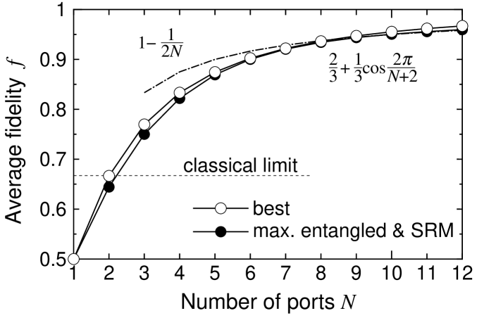
Figure 2: The average fidelity ($f$) in the deterministic scheme as a function of number of output ports ($N$). The asymptotic behavior [$1-1/(2N)$] in the case of the maximally entangled $|\psi\rangle$ is also plotted by a dash-dot line.

The above protocol of employing maximally entangled $|\psi\rangle$ and SRM can be easily extended to the case of teleporting an unknown state of a qudit ($d$-dimensional system), where $|\psi\rangle=|\phi^{+}\rangle^{\otimes N}$ with $|\phi^{+}\rangle=(1/\sqrt{d})\sum_{k=0}^{d-1}|kk\rangle$, and the POVM elements are given by Eq. (27) with $\sigma^{(i)}=(1/d^{N-1})P_{A_{i}B}^{+}\otimes\openone_{\bar{A}_{i}}$, where $P^{+}=|\phi^{+}\rangle\langle\phi^{+}|$. As mentioned in Ref. Ishizaka08b , the average fidelity is lower bounded as

$$f\geq 1-d(d-1)/N.$$ (31)

The proof is presented in Appendix B.

To investigate the property of the teleportation channel $\Lambda$ [Eq. (1) extended to the qudit case], let us consider the state isomorphic to the channel: $\omega_{BD}=(\Lambda\otimes\openone)P^{+}_{CD}$. Using $(U\otimes\openone)|\phi^{+}\rangle=(\openone\otimes U^{T})|\phi^{+}\rangle$, we have for $O=\openone$

$$(U_{B}\otimes U_{D}^{*})\omega_{BD}(U_{B}^{\dagger}\otimes U_{D}^{T})$$

$$=\sum_{i=1}^{N}\hbox{tr}_{AC}(U_{A_{i}}^{*}\otimes U_{C})\Pi_{iAC}(U_{A_{i}}^{T}\otimes U_{C}^{\dagger})(\sigma^{(i)}_{AB}\otimes P^{+}_{CD})$$

$$=\sum_{i=1}^{N}\hbox{tr}_{AC}(U_{A}^{*}\otimes U_{C})\Pi_{iAC}(U_{A}^{T}\otimes U_{C}^{\dagger})(\sigma^{(i)}_{AB}\otimes P^{+}_{CD}),$$

where $U_{A}$ denotes $U_{A_{1}}\otimes U_{A_{2}}\otimes\cdots\otimes U_{A_{N}}$, and $\sigma^{(i)}_{AB}=U_{\bar{A}_{i}}^{T}\sigma^{(i)}_{AB}U_{\bar{A}_{i}}^{*}$ was used in the second equality. Since $\sigma^{(i)}_{AC}$ (and thus $\rho_{AC}$) is invariant under the $(U_{A}^{*}\otimes U_{C})$-twirling, $\{\Pi_{iAC}\}$ of SRM (and $\Delta_{AC}$) is also invariant under the twirling. As a result, $\omega_{BD}$ is invariant under the $(U_{B}\otimes U_{D}^{*})$-twirling. This implies that $\omega_{BD}$ is an isotropic state, and therefore the teleportation channel is a depolarizing channel.

IV.2 Optimal $|\psi\rangle$

Let us next consider the case where both $|\psi\rangle$ and Alice’s measurement are optimized. The optimal POVM elements are

$$\tilde{\Pi}_{i}=\sum_{s=s_{\rm min}}^{(N-1)/2}z(s)\rho(s)^{-1/y(s)}\sigma^{(i)}(s)\rho(s)^{-1/y(s)},$$ (32)

where $y(s)$ is defined through

$$\bigg{(}\frac{\lambda_{s-1/2}^{-}}{\lambda_{s+1/2}^{+}}\bigg{)}^{1/y(s)}\frac{s+1}{s}=\sin\frac{2\pi(s+1)}{N+2}/\sin\frac{2\pi s}{N+2}\equiv D(s),$$ (33)

and $z(s)$ is given by

$$z(s)=\frac{2^{N+1}\big{(}\lambda_{s-1/2}^{-}\big{)}^{2/y(s)-1}}{(N+2)sg^{[N]}(s-1/2)}\sin^{2}\frac{2\pi s}{N+2}.$$

Note that the form of the optimal $\tilde{\Pi}_{i}$ resembles the form of SRM, but $y(s)$ is not generally equal to 2; it is a function of $s$ (and $N$). In this way, the optimal measurement becomes, say, the generalized SRM if both $|\psi\rangle$ and Alice’s measurement are optimized. Note further that we implicitly assume that the excess term $\tilde{\Delta}$ is added to every $\tilde{\Pi}_{i}$, as in the case of SRM, so that the POVM elements sum to $X\otimes\openone$ [see Eq. (4)]. The optimal state $|\psi\rangle$ is specified through $X$ given by

$$X=\sum_{j=j_{\rm min}}^{N/2}\gamma(j)\openone(j)_{A},$$ (34)

where $\openone(j)_{A}$ is the identity on the subspace spanned by $|\Phi^{[N]}(j,\cdots)\rangle_{A}$, and

$$\gamma(j)=\frac{2^{N+2}}{(N+2)(2j+1)g^{[N]}(j)}\sin^{2}\frac{\pi(2j+1)}{N+2}.$$ (35)

For the above choice of $\{\tilde{\Pi}_{i}\}$,

$$\sum_{i=1}^{N}\tilde{\Pi}_{i}= \sum_{s=s_{\rm min}}^{(N-1)/2}z(s)\rho(s)^{1-2/y(s)}$$

$$= z(s_{\rm min})\big{(}\lambda_{s_{\rm min}-1/2}^{-}\big{)}^{1-2/y(s_{\rm min})}\openone_{-}(s_{\rm min})$$

$$+\sum_{s=s_{\rm min}+1}^{(N-1)/2}\Big{\{}z(s)\big{(}\lambda_{s-1/2}^{-}\big{)}^{1-2/y(s)}\openone_{-}(s)$$

$$\quad+z(s-1)\big{(}\lambda_{s-1/2}^{+}\big{)}^{1-2/y(s-1)}\openone_{+}(s-1)\Big{\}}$$

$$+z({\textstyle\frac{N-1}{2}})\big{(}\lambda_{N/2}^{+}\big{)}^{1-2/y({\textstyle\frac{N-1}{2}})}\openone_{+}({\textstyle\frac{N-1}{2}}),$$

where

$$\openone_{\mp}(s)=\sum_{m=-s}^{s}\sum_{\alpha}|\Psi(\lambda_{s\mp 1/2}^{\mp};m)\rangle\langle\Psi(\lambda_{s\mp 1/2}^{\mp};m)|$$ (36)

is the identity on the support of $\rho_{\mp}(s)$ [see Eq. (17)]. Using

$$z(s)\big{(}\lambda_{s-1/2}^{-}\big{)}^{1-2/y(s)} =z(s-1)\big{(}\lambda_{s-1/2}^{+}\big{)}^{1-2/y(s-1)}$$

$$=\gamma(s-1/2),$$ (37)

and the following relation:

$$\openone_{-}(s)+\openone_{+}(s-1)=\openone(s-{\textstyle\frac{1}{2}})_{A}\otimes\openone_{B}$$ (38)

obtained from Eq. (III) and the CG coefficients, we have

$$\sum_{i=1}^{N}\tilde{\Pi}_{i}= \sum_{j=j_{\rm min}}^{N/2-1}\gamma(j)\openone(j)_{A}\otimes\openone_{B}+\gamma({\textstyle\frac{N}{2}})\openone_{+}({\textstyle\frac{N-1}{2}})$$

$$\leq X_{A}\otimes\openone_{B}.$$ (39)

Therefore, the constraint of Eq. (4) can be satisfied for an appropriate choice of $\tilde{\Delta}\geq 0$. Moreover, since

$$\hbox{tr}X=\frac{2^{N+2}}{N+2}\sum_{j=j_{\rm min}}^{N/2}\sin^{2}\frac{\pi(2j+1)}{N+2}=2^{N},$$ (40)

the constraint of Eq. (5) is also satisfied.

The optimal entanglement fidelity is then calculated as

$$F= \frac{1}{2^{N+1}}\hbox{tr}\sum_{s=s_{\rm min}}^{(N-1)/2}z(s)c(s,y(s))\rho(s)^{1-1/y(s)}$$

$$= \frac{1}{(N+2)}\sum_{s=s_{\rm min}}^{(N-1)/2}\frac{\sin^{2}\frac{2\pi s}{N+2}}{sg^{[N]}(s-1/2)}\Big{[}D(s)+1\Big{]}$$

$$\times\Big{[}D(s)\frac{s^{2}}{s+1}\frac{\lambda_{s+1/2}^{+}}{\lambda_{s-1/2}^{-}}g^{[N]}(s+1/2)+sg^{[N]}(s-1/2)\Big{]}$$

$$= \frac{1}{(N+2)}\sum_{s=s_{\rm min}}^{(N-1)/2}\sin^{2}\frac{2\pi s}{N+2}\Big{[}D(s)+1\Big{]}^{2}$$

$$= \cos^{2}\frac{\pi}{N+2},$$ (41)

where $D(s)$ has been defined in Eq. (33). The corresponding average fidelity

$$f=\frac{2}{3}+\frac{1}{3}\cos\frac{2\pi}{N+2}$$ (42)

is plotted by open circles in Fig. 2. The optimality of Eq. (41) is proved in Appendix C. Since both $|\psi\rangle$ and Alice’s measurement are simultaneously optimized, this is the best fidelity in the teleportation scheme such that Bob simply selects one of the multiple qubits. It is found from the figure that the best fidelity is nearly achieved by the protocol of employing maximally entangled $|\psi\rangle$ and SRM. Note, however, that the asymptotic behaviors of the fidelity are different from each other: $f\rightarrow 1-{\cal O}(1/N)$ for maximally entangled $|\psi\rangle$ [Eq. (30)], while $f\rightarrow 1-{\cal O}(1/N^{2})$ if $|\psi\rangle$ is also optimized [Eq. (42)].

V Probabilistic version

In the probabilistic scheme, the teleportation sometimes fails, but if the teleportation succeeds, the state is faithfully teleported with perfect fidelity $f=1$. The optimal protocol is then such that it maximizes the average success probability.

Let $\{\Pi_{0},\Pi_{1},\Pi_{2},\cdots,\Pi_{N}\}$ be the POVM elements of Alice’s measurement. Suppose that the teleportation fails if $\Pi_{0}$ is obtained in her measurement; otherwise, when $\Pi_{i}$ with $i\neq 0$ is obtained, the teleportation faithfully succeeds, where the state of the $B_{i}$ qubit is exactly equal to the input state of the $C$ qubit (see Fig. 1). As in the case of the deterministic version discussed in Sec. II, the teleportation channel is given by Eq. (1) (when the teleportation succeeds). However, the channel is trace-nonpreserving in this case, and

$$\hbox{tr}\Lambda(\sigma^{\rm in})=\frac{1}{2^{N}}\sum_{i=1}^{N}\hbox{tr}_{AC}\Pi_{iAC}\left(OO^{\dagger}\otimes\sigma^{\rm in}_{C}\right)$$ (43)

corresponds to the success probability (when the input state is $\sigma^{\rm in}$). The success probability $p$ averaged over all uniformly distributed input pure states is then given by

$$p=\frac{1}{2^{N}}\sum_{i=1}^{N}\hbox{tr}\Pi_{i}(OO^{\dagger}\otimes\frac{\openone_{C}}{2})=\frac{1}{2^{N+1}}\sum_{i=1}^{N}\hbox{tr}\tilde{\Pi}_{i},$$ (44)

where we again introduced $\tilde{\Pi}_{i}=(O^{\dagger}\otimes\openone)\Pi_{i}(O\otimes\openone)$. Note that $p$ agrees with the success probability when half of $P^{-}_{CD}$ is teleported as in the entanglement swapping. The entanglement fidelity is thus given by

$$F=\frac{1}{p}\hbox{tr}P^{-}_{BD}\left[(\Lambda\otimes\openone)P^{-}_{CD}\right]=\frac{1}{2^{2}p}\sum_{i=1}^{N}\hbox{tr}\tilde{\Pi}_{iAB}\sigma^{(i)}_{AB}.$$

Since $F=1$ for the faithful teleportation, it is found that $\hbox{tr}\tilde{\Pi}_{i}(\openone-P^{-})_{A_{i}B}=0$ must hold for $i=1,2,\cdots,N$. This implies that $\tilde{\Pi}_{i}$ must have the form of

$$\tilde{\Pi}_{i}=P^{-}_{A_{i}B}\otimes\tilde{\Theta}_{i\bar{A}_{i}}\hbox{~{}~{}for $i=1,2,\cdots,N$},$$ (45)

where $\{\tilde{\Theta}_{i}\}$ with $i=1,2,\cdots,N$ must satisfy

$$\tilde{\Theta}_{i}\geq 0\hbox{~{}~{}~{}and~{}~{}~{}}\sum_{i=1}^{N}P^{-}_{A_{i}B}\otimes\tilde{\Theta}_{i\bar{A}_{i}}\leq X_{A}\otimes\openone_{B},$$ (46)

because $\Pi_{i}\geq 0$ and $\sum_{i=1}^{N}\Pi_{i}\leq\openone$. Here, we again introduced $X=O^{\dagger}O$, which must satisfy Eq. (5). The average success probability is then written as

$$p=\frac{1}{2^{N+1}}\sum_{i=1}^{N}\hbox{tr}\tilde{\Theta}_{i\bar{A}_{i}}.$$ (47)

Therefore, the optimal protocol of the probabilistic version is obtained by maximizing $p$ given by Eq. (47) with respect to $\{\tilde{\Theta}_{i}\}$ and $X$ under the constraints of Eqs. (46) and (5).

VI Optimal success probability

VI.1 Maximally entangled $|\psi\rangle$

Let us first consider the case where the state $|\psi\rangle$ is fixed as $|\psi\rangle=|\psi^{-}\rangle^{\otimes N}$, i.e., $X=O^{\dagger}O=\openone$, and only the measurement performed by Alice is optimized to maximize the success probability $p$. The optimal POVM elements are given by

$$\tilde{\Theta}_{i\bar{A}_{i}}=\frac{1}{2^{N-1}}\sum_{s=s_{\rm min}}^{(N-1)/2}\frac{1}{\lambda_{s+1/2}^{+}}\openone(s)_{\bar{A}_{i}},$$ (48)

where $\openone(s)_{\bar{A}_{i}}$ is the identity on the subspace spanned by $|\Phi^{[N-1]}(s,\cdots)\rangle_{\bar{A}_{i}}$. For this choice,

$$\sum_{i=1}^{N}P^{-}_{A_{i}B}\otimes\tilde{\Theta}_{i\bar{A}_{i}} =\sum_{s=s_{\rm min}}^{(N-1)/2}\frac{1}{\lambda_{s+1/2}^{+}}\sum_{i=1}^{N}\frac{1}{2^{N-1}}P^{-}_{A_{i}B}\otimes\openone(s)_{\bar{A}_{i}}$$

$$=\sum_{s=s_{\rm min}}^{(N-1)/2}\frac{1}{\lambda_{s+1/2}^{+}}\rho(s)\leq\openone,$$ (49)

because $\lambda_{s+1/2}^{+}$ is the largest eigenvalue of $\rho(s)$, and hence the constraint of Eq. (46) is satisfied. The optimal success probability is then calculated as

$$p =\frac{1}{2^{2N}}\sum_{s=s_{\rm min}}^{(N-1)/2}\frac{N}{\lambda_{s+1/2}^{+}}\hbox{tr}\openone(s)_{\bar{A}_{i}}$$

$$=\frac{1}{2^{2N}}\sum_{s=s_{\rm min}}^{(N-1)/2}\frac{N(2s+1)g^{[N-1]}(s)}{\lambda_{s+1/2}^{+}}$$

$$=\frac{1}{2^{N}}\sum_{s=s_{\rm min}}^{(N-1)/2}\frac{(2s+1)^{2}N!}{(\frac{N-1}{2}-s)!(\frac{N+3}{2}+s)!},$$ (50)

which is plotted by closed circles in Fig. 3. Moreover, we find

$$p\rightarrow 1-\sqrt{8/(\pi N)}\hbox{~{}~{}~{}for $N\rightarrow\infty$},$$ (51)

and therefore, this protocol achieves the unit success probability in the asymptotic limit of $N\rightarrow\infty$. The optimality of Eq. (50) is proved in Appendix D.

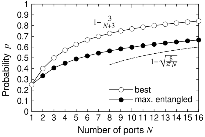
Figure 3: The average success probability ($p$) in the probabilistic scheme as a function of number of output ports ($N$). The asymptotic behavior [$1-\sqrt{8/(\pi N)}$] in the case of the maximally entangled $|\psi\rangle$ is also plotted by a dash-dot line.

VI.2 Optimal $|\psi\rangle$

Let us next consider the case where both $|\psi\rangle$ and Alice’s measurement are optimized simultaneously. The optimal POVM elements are given by

$$\tilde{\Theta}_{i\bar{A}_{i}}=\sum_{s=s_{\rm min}}^{(N-1)/2}u(s)\openone(s)_{\bar{A}_{i}},$$ (52)

where

$$u(s)=\frac{2^{N+1}h(N)(2s+1)}{Ng^{[N-1]}(s)}$$ (53)

with $h(N)=6/[(N+1)(N+2)(N+3)]$. The optimal state $|\psi\rangle$ is specified through $X$ given by

$$X=\sum_{j=j_{\rm min}}^{N/2}\nu(j)\openone(j)_{A}\hbox{~{}with~{}}\nu(j)=\frac{2^{N}h(N)(2j+1)}{g^{[N]}(j)}.$$ (54)

For the above choice,

$$\frac{1}{2^{N-1}}\sum_{i=1}^{N}P^{-}_{A_{i}B}\otimes\tilde{\Theta}_{i\bar{A}_{i}}=\sum_{s=s_{\rm min}}^{(N-1)/2}u(s)\rho(s)$$

$$= u(s_{\rm min})\lambda_{s_{\rm min}-1/2}^{-}\openone_{-}(s_{\rm min})$$

$$+ \sum_{s=s_{\rm min}+1}^{(N-1)/2}\Big{\{}u(s)\lambda_{s-1/2}^{-}\openone_{-}(s)$$

$$+ u(s-1)\lambda_{s-1/2}^{+}\openone_{+}(s-1)\Big{\}}+u({\textstyle\frac{N-1}{2}})\lambda_{N/2}^{+}\openone_{+}({\textstyle\frac{N-1}{2}}),$$

where $\openone_{\mp}(s)$ is given by Eq. (36). Using

$$u(s)\lambda_{s-1/2}=u(s-1)\lambda_{s-1/2}=\nu(s-1/2)/2^{N-1},$$

and Eq. (38), the fulfillment of Eq. (46) is confirmed in the same way as Eq. (39). The constraint of Eq. (5) is also satisfied because

$$\hbox{tr}X=2^{N}h(N)\sum_{j=j_{\rm min}}^{N/2}(2j+1)^{2}=2^{N}.$$ (55)

The optimal success probability is then

$$p =\frac{N}{2^{N+1}}\sum_{s=s_{\rm min}}^{(N-1)/2}u(s)\hbox{tr}\openone(s)_{\bar{A}_{i}}$$

$$=h(N)\sum_{s=s_{\rm min}}^{(N-1)/2}(2s+1)^{2}=\frac{N}{N+3}=1-\frac{3}{N+3},$$ (56)

which is plotted by open circles in Fig. 3. The optimality of Eq. (56) is proved in Appendix E. Here, let us recall that the success probability in the KLM scheme is equal to $p=1-1/(N+1)$ Knill01a . Comparing this and Eq. (56), it is found that the number of ports $N$ in our scheme must be just three times larger than that of the KLM scheme to achieve the same success probability. Therefore, this three times increase of the number of ports is, in some sense, regarded as the cost we have to pay to remove Bob’s unitary transformation.

It has been shown in Ref. Grudka08a that the success probability of the (probabilistic) KLM scheme is maximized when a maximally entangled state is employed. On the other hand, in contrast to the KLM scheme, the success probability in our scheme is considerably enhanced by optimizing $|\psi\rangle$ as shown in Fig. 3. This implies that non-maximally entangled $|\psi\rangle$ can provide considerably larger success probability than that of a maximally entangled $|\psi\rangle$. Interestingly, we have from Eq. (54)

$$\sigma_{B_{i}} =\hbox{tr}_{A\bar{B}_{i}}|\psi\rangle\langle\psi|=\frac{1}{2^{N}}\sigma_{2}\big{(}\hbox{tr}_{\bar{B}_{i}}X^{T}_{B_{1}\cdots B_{N}}\big{)}\sigma_{2}$$

$$=\frac{1}{2^{N}}\sum_{j=j_{\rm min}}^{N/2}\nu(j)(2j+1)g^{[N]}(j)\frac{\openone_{B_{i}}}{2}=\frac{\openone_{B_{i}}}{2}.$$

Namely, although the optimal $|\psi\rangle$ is non-maximally entangled in the $A_{1}A_{2}\cdots A_{N}:B_{1}B_{2}\cdots B_{N}$ cut, each $B_{i}$ qubit is still maximally entangled with the other qubits, with both $A$ and $\bar{B}_{i}$ qubits, in a complicated manner. Note that this is also the case for the optimal $|\psi\rangle$ in the deterministic version discussed in Sec. IV.2; we have $\sigma_{B_{i}}=\openone/2$ by using Eq. (34), although the optimal fidelity is nearly achieved by the maximally entangled $|\psi\rangle$ as was shown in Fig. 2, in constrast to the success probability.

VII Example

Now, let us show the explicit form of the optimal $|\psi\rangle$ and the optimal POVM elements of Alice’s measurement in the simplest case of $N=2$ in the probabilistic scheme. From Eq. (56), the optimal success probability in this case is $p=2/5$. From Eq. (54) for $N=2$, we have

$$X =\frac{2}{5}\openone(0)_{A}+\frac{6}{5}\openone(1)_{A}$$

$$=\frac{2}{5}|\psi^{-}\rangle\langle\psi^{-}|+\frac{6}{5}\Big{(}|00\rangle\langle 00|+|11\rangle\langle 11|+|\psi^{+}\rangle\langle\psi^{+}|\Big{)},$$

where $A=A_{1}A_{2}$ and $|\psi^{\pm}\rangle=(|01\rangle\pm|10\rangle)/\sqrt{2}$. The optimal $|\psi\rangle$ is thus

$$|\psi\rangle =\sqrt{\frac{1}{10}}|\psi^{-}\rangle_{A}|\psi^{-}\rangle_{B_{1}B_{2}}$$

$$+\sqrt{\frac{3}{10}}\Big{(}|00\rangle|11\rangle+|11\rangle|00\rangle-|\psi^{+}\rangle|\psi^{+}\rangle\Big{)}_{AB_{1}B_{2}}.$$ (57)

From Eq. (52) for $N=2$, we have $\tilde{\Theta}_{1}=(4/5)\openone_{A_{2}}$, and hence

$$\Pi_{1} =\sqrt{X^{-1}}(P^{-}_{A_{1}C}\otimes\tilde{\Theta}_{1A_{2}})\sqrt{X^{-1}}$$

$$=\Big{(}|\eta^{-}\rangle\langle\eta^{-}|+|\eta^{+}\rangle\langle\eta^{+}|\Big{)}_{AC},$$ (58)

where $\{|\eta^{-}\rangle,|\eta^{+}\rangle\}$ are orthogonal states given by

$$|\eta^{-}\rangle_{AC}=\sqrt{\frac{2}{3}}|x^{-}\rangle_{A}|0\rangle_{C}+\sqrt{\frac{1}{3}}|00\rangle_{A}|1\rangle_{C},$$

$$|\eta^{+}\rangle_{AC}=\sqrt{\frac{2}{3}}|x^{+}\rangle_{A}|1\rangle_{C}-\sqrt{\frac{1}{3}}|11\rangle_{A}|0\rangle_{C},$$

with $|x^{\pm}\rangle=(1/2)(\pm|\psi^{+}\rangle+\sqrt{3}|\psi^{-}\rangle)$. The POVM element $\Pi_{2}$ is given by $A_{1}\leftrightarrow A_{2}$ in Eq. (58) [and thus, only $|x^{\pm}\rangle$ is replaced with $(1/2)(\pm|\psi^{+}\rangle-\sqrt{3}|\psi^{-}\rangle)$]. It is then easily confirmed that

$$\langle\eta^{-}|\Big{[}|\psi\rangle\otimes\big{(}a|0\rangle+b|1\rangle\big{)}_{C}\Big{]} =\frac{1}{\sqrt{10}}\big{(}a|0\rangle+b|1\rangle\big{)}_{B_{1}}|1\rangle_{B_{2}},$$

$$\langle\eta^{+}|\Big{[}|\psi\rangle\otimes\big{(}a|0\rangle+b|1\rangle\big{)}_{C}\Big{]} =\frac{-1}{\sqrt{10}}\big{(}a|0\rangle+b|1\rangle\big{)}_{B_{1}}|0\rangle_{B_{2}},$$

and hence

$$\sqrt{\Pi_{1}}|\psi\rangle\otimes\big{(}a|0\rangle+b|1\rangle\big{)}_{C}=\frac{1}{\sqrt{5}}|\psi_{\rm res}\rangle\otimes\big{(}a|0\rangle+b|1\rangle\big{)}_{B_{1}}.$$

Therefore, the state of the $C$ qubit is certainly teleported to the $B_{1}$ qubit faithfully, when Alice obtains $\Pi_{1}$ in her measurement (the coefficient on the right hand side represents the success probability of $p/N=1/5$). Here,

$$|\psi_{\rm res}\rangle =\frac{1}{\sqrt{2}}\Big{(}|\eta^{-}\rangle_{AC}|1\rangle_{B_{2}}-|\eta^{+}\rangle_{AC}|0\rangle_{B_{2}}\Big{)}$$

$$=\frac{1}{\sqrt{2}}|\psi^{-}\rangle_{A}|\psi^{-}\rangle_{CB_{2}}$$

$$+\frac{1}{\sqrt{6}}\Big{(}|00\rangle|11\rangle+|11\rangle|00\rangle-|\psi^{+}\rangle|\psi^{+}\rangle\Big{)}_{ACB_{2}}$$ (59)

is the residual state after the teleportation is successfully completed.

VIII Entanglement consumption

Here, let us briefly discuss the entanglement properties in the probabilistic scheme. In the explicit example for $N=2$ shown in the previous section, Alice and Bob initially share the state $|\psi\rangle$ given by Eq. (57). Using $\sigma_{A}=\hbox{tr}_{B_{1}B_{2}}|\psi\rangle\langle\psi|$, the amount of the entanglement of $|\psi\rangle$ is calculated to be $E_{\rm ini}=-\hbox{tr}\sigma_{A}\log_{2}(\sigma_{A})\approx 1.90$ ebits (entanglement bits), which is less than the possible maximal amount of 2 ebits for $N=2$ (the optimal $|\psi\rangle$ is non-maximally entangled as mentioned in Sec. VI). When Alice obtains $\Pi_{1}$ in her measurement, the state of the $C$ qubit is faithfully teleported to the $B_{1}$ qubit, i.e., the $B_{1}$ qubit is used for receiving the teleported state. However, Bob still has the $B_{2}$ qubit, and as a result, Alice and Bob still share the residual state $|\psi_{\rm res}\rangle_{ACB_{2}}$ given by Eq. (59) after the teleportation is completed. The entanglement of $|\psi_{\rm res}\rangle$ (in the $AC:B_{2}$ cut) is calculated to be just $E_{\rm res}=1$ ebit. Therefore, when the teleportation succeeds, only $E_{\rm ini}-E_{\rm res}=0.90$ ebits are violated (or consumed), in spite that a state of a single qubit is faithfully teleported. Figure 4 shows such a comparison for general $N$, where the entanglement of $|\psi\rangle$ and $|\psi_{\rm res}\rangle$ is plotted by circles and rectangles, respectively. It is found from the figure that the entanglement consumption is less than 1 ebit even for $N>2$; rather, the amount of the consumption gradually decreases for increasing $N$ ($\approx 0.52$ ebits for $N=50$).

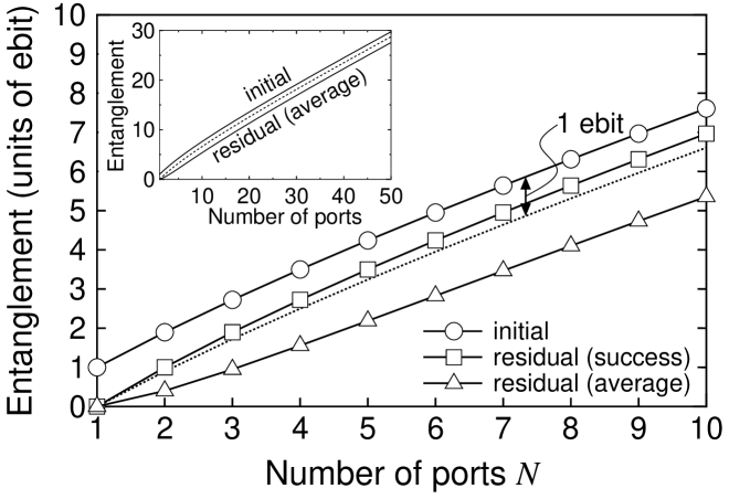
Figure 4: The amount of entanglement as a function of number of output ports ($N$) in the probabilistic scheme. The initial amount of the optimal $|\psi\rangle$ (circles), the residual amount when the teleportation is successfully finished (rectangles), and the average residual amount (triangles) are plotted. The dotted line shows the eye-guide that corresponds to the entanglement consumption by 1 ebit. The inset shows the same comparison of the initial and average residual amount up to $N=50$.

This implies that the entanglement between Alice and Bob even increases if they try to teleport half of a maximally entangled state as in the entanglement swapping (and if the teleportation is successfully finished). This is because Alice and Bob newly share 1 ebit by the entanglement swapping, while the entanglement consumption is less than 1 ebit as shown above. For this peculiar feature in our probabilistic teleportation scheme, the use of the optimal $|\psi\rangle$ is crucial; if $|\psi\rangle$ is fixed to a maximally entangled state as discussed in Sec. VI.1, we have $E_{\rm ini}=N$ and $E_{\rm res}\leq N-1$ because the number of Bob’s qubits involved in $|\psi_{\rm res}\rangle$ is $(N-1)$, and hence the entanglement consumption in this case always satisfies $E_{\rm ini}-E_{\rm res}\geq 1$ (in fact, $E_{\rm ini}-E_{\rm res}\approx 1.009$ and 1.004 for $N=10$ and $N=50$, respectively). Note that the peculiar feature of the increase of entanglement, of course, does not contradict the laws of entanglement, because the scheme discussed here is the probabilistic one and the probabilistic increase of entanglement by local operations and classical communication (LOCC) has not been prohibited by the laws of entanglement.

Let us then evaluate the average amount of the residual entanglement. When Alice obtains $\Pi_{0}$, the teleportation fails where the residual state generally depends on the input state to be teleported. Moreover, if the input state is a mixed state, the residual state is also a mixed state. Since the evaluation of the entanglement for such a mixed state is a very hard task, let us consider the worst case where the entanglement of the residual state when the teleportation fails is regarded to be zero. Using the success probability $p$ of Eq. (56), the average residual entanglement in this worst case is given by $pE_{\rm res}$, which is plotted by triangles in Fig. 4. The corresponding average amount of the entanglement consumption ($E_{\rm ini}-pE_{\rm res}$) is roughly 2.2 ebits for $N=10$, and for $N=50$ also (the inset of Fig. 4). In this way, in our probabilistic teleportation scheme, although Alice and Bob must initially share much entanglement of ${\cal O}(N)$ ebits (see the inset of Fig. 4), only a few ebits are consumed on average during the teleportation procedure. It may be said that the most of the initial entanglement is only used as a working space.

IX Summary

In this paper, we have considered the scheme of quantum teleportation, where Bob has multiple ($N$) output ports and obtains the teleported state by simply selecting one of the $N$ ports. We investigated both deterministic version and probabilistic version of the teleportation scheme aiming to teleport an unknown state of a qubit, and analytically determined the optimal protocols. All protocols shown in this paper can asymptotically achieve the perfect teleportation (i.e., faithful teleportation with unit success probability) in the limit of $N\rightarrow\infty$.

In the deterministic version of the teleportation scheme, if the state $|\psi\rangle$ employed for the teleportation is fixed to a maximally entangled state, the optimal measurement performed by Alice is the square-root measurement, where the optimal fidelity is given by Eq. (29) [or Eq. (30)]. If both $|\psi\rangle$ and Alice’s measurement are simultaneously optimized, the generalized square-root measurement becomes optimal. The optimal fidelity in this case is given by Eq. (42).

In the probabilistic version, the optimal success probability is given by Eq. (50) [or Eq. (51)] if $|\psi\rangle$ is fixed to a maximally entangled state, and given by Eq. (56) if $|\psi\rangle$ is also optimized. In contrast to the KLM scheme (and in contrast to the deterministic version of our scheme also), the success probability is considerably enhanced by optimizing $|\psi\rangle$; namely, the use of the non-maximally entangled $|\psi\rangle$ provides a considerable benefit than the use of the maximally entangled $|\psi\rangle$. Moreover, we showed that the scheme is not inefficient concerning the entanglement resource, because only a few ebits are consumed on average even for large $N$. If the optimal $|\psi\rangle$ is employed for the entanglement swapping, the amount of entanglement even increases when the teleportation is successfully completed.

Note finally that the form of the optimal fidelity Eq. (42) and the form of the optimal success probability Eq. (56) are relatively simple (although the corresponding optimal $|\psi\rangle$ and Alice’s measurement are not). Those are the achievable upper bounds in the general setting of selecting one of $N$ qubits assisted by classical communication. In this paper, those bounds were obtained by the direct optimization, but it will be important to study further how those bounds of having the simple form are related to the fundamental laws of physics. For instance, is it possible to derive those bounds only from the no-signaling condition? This seems an intriguing and important open problem.

Appendix A Proof of Eq. (13)

The proof is carried out by induction by noting that $\rho=\rho^{[N]}$ is constructed recursively;

$$\rho^{[N]}=\rho^{[N-1]}\otimes\frac{\openone_{A_{N}}}{2}+\frac{\openone_{A_{1}}}{2}\otimes\dots\otimes\frac{\openone_{A_{N-1}}}{2}\otimes P_{A_{N}B}^{-}.$$

The eigenvalue equation Eq. (13) to be proved is then rewritten as

$$\rho^{[N]}|\Psi^{[N]}(\lambda_{j}^{\mp};m)\rangle=\lambda_{j}^{\mp}|\Psi^{[N]}(\lambda_{j}^{\mp};m)\rangle,$$ (60)

where we attached a superscript $[N]$ to the eigenstates to emphasize the relevant system size. Moreover, we introduce the shorthand notation for the CG coefficients,

$$\langle j_{1},m_{1};j\rangle_{\pm}=\textstyle\langle j_{1},m_{1},\frac{1}{2},\pm\frac{1}{2}|j,m_{1}\pm\frac{1}{2}\rangle,$$

and introduce $m_{\pm}=m\pm 1/2$, $m_{\pm\pm}=m\pm 1$ and similarly for $j$.

Since Eq. (60) is obvious for $N=1$, our aim is reduced to proving Eq. (60) under the assumption that Eq. (60) with $N\rightarrow N-1$ holds true. To this end, we write $|\Psi^{[N]}\rangle$ in terms of $|\Psi^{[N-1]}\rangle$ as follows.

$$|\Psi_{\mathrm{I}}^{[N]}(\lambda_{j}^{\mp};m)\rangle$$

$$= |\Psi^{[N-1]}(\lambda_{j_{+}}^{-};m_{+})\rangle|0\rangle_{A_{N}}\big{[}\langle j_{+},m_{++};j_{++}\rangle_{-}^{*}\langle j,m_{+};j_{\pm}\rangle_{-}\langle j_{+},m_{++};j\rangle_{-}+\langle j_{+},m;j_{++}\rangle_{+}^{*}\langle j,m_{-};j_{\pm}\rangle_{+}\langle j_{+},m;j\rangle_{-}\big{]}$$

$$+ |\Psi^{[N-1]}(\lambda_{j_{+}}^{-};m_{-})\rangle|1\rangle_{A_{N}}\big{[}\langle j_{+},m;j_{++}\rangle_{-}^{*}\langle j,m_{+};j_{\pm}\rangle_{-}\langle j_{+},m;j\rangle_{+}+\langle j_{+},m_{--};j_{++}\rangle_{+}^{*}\langle j,m_{-};j_{\pm}\rangle_{+}\langle j_{+},m_{--};j\rangle_{+}\big{]}$$

$$+ |\Psi^{[N-1]}(\lambda_{j_{+}}^{+};m_{+})\rangle|0\rangle_{A_{N}}\big{[}\langle j_{+},m_{++};j\rangle_{-}^{*}\langle j,m_{+};j_{\pm}\rangle_{-}\langle j_{+},m_{++};j\rangle_{-}+\langle j_{+},m;j\rangle_{+}^{*}\langle j,m_{-};j_{\pm}\rangle_{+}\langle j_{+},m;j\rangle_{-}\big{]}$$

$$+ |\Psi^{[N-1]}(\lambda_{j_{+}}^{+};m_{-})\rangle|1\rangle_{A_{N}}\big{[}\langle j_{+},m;j\rangle_{-}^{*}\langle j,m_{+};j_{\pm}\rangle_{-}\langle j_{+},m;j\rangle_{+}+\langle j_{+},m_{--};j\rangle_{+}^{*}\langle j,m_{-};j_{\pm}\rangle_{+}\langle j_{+},m_{--};j\rangle_{+}\big{]},$$ (61)

and

$$|\Psi_{\mathrm{II}}^{[N]}(\lambda_{j}^{\mp};m)\rangle$$

$$= |\Psi^{[N-1]}(\lambda_{j_{-}}^{-};m_{+})\rangle|0\rangle_{A_{N}}\big{[}\langle j_{-},m_{++};j\rangle_{-}^{*}\langle j,m_{+};j_{\pm}\rangle_{-}\langle j_{-},m_{++};j\rangle_{-}+\langle j_{-},m;j\rangle_{+}^{*}\langle j,m_{-};j_{\pm}\rangle_{+}\langle j_{-},m;j\rangle_{-}\big{]}$$

$$+ |\Psi^{[N-1]}(\lambda_{j_{-}}^{-};m_{-})\rangle|1\rangle_{A_{N}}\big{[}\langle j_{-},m;j\rangle_{-}^{*}\langle j,m_{+};j_{\pm}\rangle_{-}\langle j_{-},m;j\rangle_{+}+\langle j_{-},m_{--};j\rangle_{+}^{*}\langle j,m_{-};j_{\pm}\rangle_{+}\langle j_{-},m_{--};j\rangle_{+}\big{]}$$

$$+ |\Psi^{[N-1]}(\lambda_{j_{-}}^{+};m_{+})\rangle|0\rangle_{A_{N}}\big{[}\langle j_{-},m_{++};j_{--}\rangle_{-}^{*}\langle j,m_{+};j_{\pm}\rangle_{-}\langle j_{-},m_{++};j\rangle_{-}+\langle j_{-},m;j_{--}\rangle_{+}^{*}\langle j,m_{-};j_{\pm}\rangle_{+}\langle j_{-},m;j\rangle_{-}\big{]}$$

$$+ |\Psi^{[N-1]}(\lambda_{j_{-}}^{+};m_{-})\rangle|1\rangle_{A_{N}}\big{[}\langle j_{-},m;j_{--}\rangle_{-}^{*}\langle j,m_{+};j_{\pm}\rangle_{-}\langle j_{-},m;j\rangle_{+}+\langle j_{-},m_{--};j_{--}\rangle_{+}^{*}\langle j,m_{-};j_{\pm}\rangle_{+}\langle j_{-},m_{--};j\rangle_{+}\big{]}.$$ (62)

Equations (A) and (A) are obtained by calculating the overlap between $|\Psi_{\mathrm{I}(\mathrm{II})}^{[N]}\rangle$ given by Eqs. (III) and (III) and $|\Psi^{[N-1]}\rangle$ given by Eq. (III) with $N\rightarrow N-1$.

The vector $\rho^{[N-1]}\otimes\openone_{A_{N}}|\Psi_{\mathrm{I}(\mathrm{II})}^{[N]}(\lambda_{j}^{\mp};m)\rangle$ takes the form of the right hand side of Eqs. (A) and (A) with

$$|\Psi^{[N-1]}(\lambda_{j_{+}}^{\mp};\dots)\rangle\rightarrow\lambda_{j_{+}}^{[N-1]\mp}|\Psi^{[N-1]}(\lambda_{j_{+}}^{[N-1]\mp};\dots)\rangle,$$

$$|\Psi^{[N-1]}(\lambda_{j_{-}}^{\mp};\dots)\rangle\rightarrow\lambda_{j_{-}}^{[N-1]\mp}|\Psi^{[N-1]}(\lambda_{j_{-}}^{[N-1]\mp};\dots)\rangle,$$

and these are further written in terms of $|\Phi^{[N-1]}\rangle$. Here, we again attached a superscript $[N]$ to eigenvalues $\lambda^{\mp}_{j}$ to emphasize the relevant system size. On the other hand, the vector $\openone_{\bar{A}_{N}}\otimes P_{BA_{N}}^{-}|\Psi_{\mathrm{I}(\mathrm{II})}^{[N]}(\lambda_{j}^{\mp};m)\rangle$ takes the form of the right hand side of Eqs. (III) and (III) with

$$|0\rangle_{B}|1\rangle_{A_{N}} \rightarrow(|0\rangle_{B}|1\rangle_{A_{N}}-|1\rangle_{B}|0\rangle_{A_{N}})/\sqrt{2},$$

$$|1\rangle_{B}|0\rangle_{A_{N}} \rightarrow-(|0\rangle_{B}|1\rangle_{A_{N}}-|1\rangle_{B}|0\rangle_{A_{N}})/\sqrt{2}.$$

Putting these two results together (and after lengthy calculations), we can see the desired eigenvalue equation,

$$\rho^{[N]}|\Psi_{\mathrm{I}(\mathrm{II})}^{[N]}(\lambda_{j}^{\mp};m)\rangle$$

$$= \Big{(}\rho^{[N-1]}\otimes\frac{\openone_{A_{N}}}{2}+\frac{\openone_{\bar{A}_{N}}}{2^{N-1}}\otimes P_{A_{N}B}^{-}\Big{)}|\Psi_{\mathrm{I}(\mathrm{II})}^{[N]}(\lambda_{j}^{\mp};m)\rangle$$

$$= \lambda_{j}^{\mp}|\Psi_{\mathrm{I}(\mathrm{II})}^{[N]}(\lambda_{j}^{\mp};m)\rangle.$$

This completes the proof.

Appendix B Proof of Eq. (31)

The proof is based on the technique used in the Holeve-Schumacher-Westmoreland (HSW) theorem Holevo98a ; Schmacher97a . Let us denote the eigenstates of $\sigma^{(i)}$ by $|k^{(i)}\rangle$, and hence $\sigma^{(i)}=(1/d^{N-1})\sum_{k}|k^{(i)}\rangle\langle k^{(i)}|$. The entanglement fidelity then satisfies

$$F =\frac{1}{d^{2}}\hbox{tr}\sum_{i=1}^{N}\rho^{-1/2}\sigma^{(i)}\rho^{-1/2}\sigma^{(i)}$$

$$\geq\frac{1}{d^{2N}}\sum_{i=1}^{N}\sum_{k}|\langle k^{(i)}|\rho^{-1/2}|k^{(i)}\rangle|^{2}$$

$$=\frac{1}{Nd^{N-1}}\sum_{i=1}^{N}\sum_{k}|\langle k^{(i)}|\Big{(}d^{N+1}\rho/N\Big{)}^{-1/2}|k^{(i)}\rangle|^{2}$$

$$\geq\frac{2}{Nd^{N-1}}\sum_{i=1}^{N}\sum_{k}\langle k^{(i)}|\Big{(}d^{N+1}\rho/N\Big{)}^{-1/2}|k^{(i)}\rangle-1$$

$$=\frac{2}{d^{N+1}}\hbox{tr}\Big{(}d^{N+1}\rho/N\Big{)}^{1/2}-1\geq 2-\frac{d^{N+1}}{N^{2}}\hbox{tr}\rho^{2}$$

where $x^{2}\geq 2x-1$ was used in the second inequality, and $2(\openone-\Gamma^{1/2})\leq 2\openone-3\Gamma+\Gamma^{2}$ was used in the last inequality Holevo98a ; Schmacher97a ; NielsenChuang . Since

$$\hbox{tr}\rho^{2}=\frac{1}{d^{N-1}}\sum_{i,j=1}^{N}\langle k^{(i)}|\sigma^{(j)}|k^{(i)}\rangle=\frac{N}{d^{N-1}}+\frac{N(N-1)}{d^{N+1}},$$

we have $F\geq 1-(d^{2}-1)/N$, and thus Eq. (31), because $f=(Fd+1)/(d+1)$ Horodecki99a .

Appendix C Optimality of Eq. (42)

The problem of maximizing $F$ given by Eq. (3) under the constraints of Eqs. (4) and (5) is a semidefinite program Boyd04a and thus has the dual problem. Since the Lagrange function is

$${\cal L} =\sum_{i=1}^{N}\hbox{tr}\tilde{\Pi}_{i}\sigma^{(i)}-\hbox{tr}\Omega\Big{(}\sum_{i=1}^{N}\tilde{\Pi}_{i}\!-\!X\otimes\openone\Big{)}-a(\hbox{tr}X\!-\!2^{N})$$

$$=2^{N}a-\sum_{i=1}^{N}\hbox{tr}\tilde{\Pi}_{i}(\Omega\!-\!\sigma^{(i)})-\hbox{tr}X(a\openone\!-\!\hbox{tr}_{B}\Omega),$$

where $\Omega$ and $a$ are the Lagrange multipliers, the dual problem is of minimizing $F=2^{N-2}a$ subject to

$$a\openone_{A}-\hbox{tr}_{B}\Omega\geq 0,\hbox{~{}~{}}\Omega-\sigma^{(i)}\geq 0.$$ (63)

Let us take

$$a =\frac{1}{2^{N-2}}\cos^{2}\frac{\pi}{N+2},$$

$$\Omega =\frac{1}{2^{N-1}}\sum_{s=s_{\rm min}}^{(N-1)/2}c(s,y(s))\rho(s)^{1/y(s)}.$$

Since any feasible solution of the dual problem gives an upper bound of the original problem Boyd04a , and $F=2^{N-2}a$ agrees with Eq. (41), it is then enough to show that the above $\Omega$ is a feasible solution, i.e., $\Omega$ satisfies the constraints of Eq. (63). It is found from Eq. (III) and the CG coefficients that

$$2^{N-1}\hbox{tr}_{B}\Omega=$$

$$c(s_{\rm min})\big{(}\lambda_{s_{\rm min}-1/2}^{-}\big{)}^{1/y(s_{\rm min})}\frac{2s_{\rm min}+1}{2s_{\rm min}}\openone(s_{\rm min}-{\textstyle\frac{1}{2}})_{A}$$

$$+ \sum_{s=s_{\rm min}+1}^{(N-1)/2}\Big{\{}c(s)\big{(}\lambda_{s-1/2}^{-}\big{)}^{1/y(s)}\frac{2s+1}{2s}$$

$$\quad+c(s-1)\big{(}\lambda_{s-1/2}^{+}\big{)}^{1/y(s-1)}\frac{2s-1}{2s}\Big{\}}\openone(s-{\textstyle\frac{1}{2}})_{A}$$

$$+ c({\textstyle\frac{N-1}{2}})\big{(}\lambda_{N/2}^{+}\big{)}^{1/y({\textstyle\frac{N-1}{2}})}\frac{N}{N+1}\openone({\textstyle\frac{N}{2}})_{A},$$

where $c(s)\equiv c(s,y(s))$ and $\openone(j)$ is the identity on the subspace spanned by $|\Phi^{[N]}(j,\cdots)\rangle$. Since

$$c(s)\big{(}\lambda_{s-1/2}^{-}\big{)}^{1/y(s)}\frac{2s+1}{2s}$$

$$+c(s-1)\big{(}\lambda_{s-1/2}^{+}\big{)}^{1/y(s-1)}\frac{2s-1}{2s}$$

$$\quad=1+\frac{D(s)}{2}+\frac{1}{2D(s-1)}=2\cos^{2}\frac{2\pi}{N+2},$$

we have $\hbox{tr}_{B}\Omega=a\openone_{A}$, and hence the first constraint in Eq. (63) is satisfied. Moreover, in the same way as in Ref. Ishizaka08b ,

$$\rho(s)^{1/y(s)}-\frac{1}{c(s,y(s))}\sum_{m,\beta}|\xi^{(i)}(s,m,\beta)\rangle\langle\xi^{(i)}(s,m,\beta)|\geq 0$$

follows from Eq. (25), and thus the second constraint in Eq. (63) is also satisfied.

Appendix D Optimality of Eq. (50)

The problem of maximizing $p$ given by Eq. (47) under the constraints of Eqs. (46) (with fixed $X=\openone$) is also a semidefinite program. The dual problem is of minimizing $p=(1/2^{N+1})\hbox{tr}\Omega$ subject to

$$\Omega\geq 0,\hbox{~{}~{}}\hbox{tr}_{A_{i}B}P^{-}_{A_{i}B}\Omega_{AB}\geq\openone_{\bar{A}_{i}}.$$ (64)

For the choice of

$$\Omega=\sum_{s=s_{\rm min}}^{(N-1)/2}\frac{2s+1}{s+1}\sum_{m,\beta}|\Psi(\lambda_{s+1/2}^{+};m)\rangle\langle\Psi(\lambda_{s+1/2}^{+};m)|,$$

it is found from Eqs. (22) and (III) that

$$\hbox{tr}_{A_{i}B}P^{-}_{BA_{i}}\Omega=\sum_{s=s_{\rm min}}^{(N-1)/2}\frac{2s+1}{s+1}\frac{s+1}{2s+1}\openone(s)_{\bar{A}_{i}}=\openone_{\bar{A}_{i}},$$

and therefore the above $\Omega$ is a feasible solution. On the other hand, $p=(1/2^{N+1})\hbox{tr}\Omega$ agrees with Eq. (50), because the degeneracy of $|\Psi(\lambda_{s+1/2}^{+};m)\rangle$ is $(2s+1)g^{[N]}(s+1/2)$ [see Eq. (21)] and

$$\frac{(2s+1)^{2}g^{[N]}(s+1/2)}{s+1}=\frac{N}{2^{N-1}}\frac{(2s+1)g^{[N-1]}(s)}{\lambda_{s+1/2}^{+}}.$$

Appendix E Optimality of Eq. (56)

The dual problem for general $X$ is of minimizing $p=2^{N}a$ subject to

$$\Omega\geq 0,\hbox{~{}~{}}\hbox{tr}_{A_{i}B}P^{-}_{A_{i}B}\Omega_{AB}\geq\openone_{\bar{A}_{i}},\hbox{~{}~{}}a\openone_{A}-\frac{1}{2^{N+1}}\hbox{tr}_{B}\Omega\geq 0.$$ (65)

Let us take $a=(1/2^{N})N/(N+3)$ and consider

$$\Omega=\sum_{s=s_{\rm min}}^{(N-1)/2}\sum_{m,\beta}\Big{\{} d(s)|\Psi(\lambda_{s+1/2}^{+};m)\rangle\langle\Psi(\lambda_{s+1/2}^{+};m)|$$

$$+ e(s)|\Psi(\lambda_{s-1/2}^{-};m)\rangle\langle\Psi(\lambda_{s-1/2}^{-};m)|\Big{\}},$$

where $d(s)=(N+3+2s)/(N+3)$ and $e(s)=(N+1-2s)/(N+3)$. Since $p=2^{N}a$ agrees with Eq. (56), it is enough to show that the above $\Omega$ is a feasible solution. From Eqs. (III), (20), (22), and (III), it is found that

$$\hbox{tr}_{A_{i}B}P^{-}_{A_{i}B}\Omega =\sum_{s=s_{\rm min}}^{(N-1)/2}\Big{\{}\frac{d(s)(s+1)}{2s+1}+\frac{e(s)s}{2s+1}\Big{\}}\openone(s)_{\bar{A}_{i}}$$

$$=\openone_{\bar{A}_{i}},$$

and the second constraint of Eq. (65) is satisfied. Moreover, it is found from Eq. (III) and the CG coefficients that

$$\hbox{tr}_{B}\Omega=\sum_{s=s_{\rm min}}^{(N-1)/2}\Big{\{} \frac{d(s)(2s+1)}{2(s+1)}\openone({\textstyle s+\frac{1}{2}})_{A}$$

$$+ \frac{e(s)(2s+1)}{2s}\openone({\textstyle s-\frac{1}{2}})_{A}\Big{\}}=\frac{2N}{N+3}\openone_{A},$$

and hence the third constraint of Eq. (65) is also satisfied.

References

(1)
C. H. Bennett et al., Phys. Rev. Lett. 70, 1895 (1993).
(2)
D. Bouwmeester et al., Nature (London) 390, 575 (1997).
(3)
D. Boschi, S. Branca, F. De Martini, L. Hardy, and S. Popescu, Phys. Rev. Lett. 80, 1121 (1998).
(4)
A. Furusawa et al., Science 282, 706 (1998);
S. L. Braunstein and H. J. Kimble, Nature (London) 394, 840 (1998).
(5)
S. L. Braunstein and H. J. Kimble, Phys. Rev. Lett. 80, 869 (1998);
P. van Loock and S. L. Braunstein, Phys. Rev. Lett. 84, 3482 (2000);
S. Pirandola, S. Mancini, D. Vitali, and P. Tombesi, Phys. Rev. A 68, 062317 (2003);
S. Pirandola, S. Mancini, and D. Vitali, Phys. Rev. A 71, 042326 (2005);
S. Pirandola and S. Mancini, Laser Physics 16, 1418 (2006).
(6)
M. A. Nielsen and I. L. Chuang, Phys. Rev. Lett. 79, 321 (1997).
(7)
D. Gottesman and I. L. Chuang, Nature (London) 402, 390 (1999).
(8)
J. Kim, Y. Cheong, J.-S. Lee, and S. Lee, Phys. Rev. A 65, 012302
(2001).
(9)
G. Vidal, L. Masanes, and J. I. Cirac, Phys. Rev. Lett. 88, 047905
(2002).
(10)
J. Fiurás̆ek, M. Dus̆ek, and R. Filip, Phys. Rev. Lett. 89,
190401 (2002).
(11)
J. Fiurás̆ek and M. Dus̆ek, Phys. Rev. A 69, 032302 (2004).
(12)
A. Brazier, V. Buz̆ek, and P. L. Knight, Phys. Rev. A 71, 032306
(2005).
(13)
M. Ziman and V. Buz̆ek, Phys. Rev. A 72, 022343 (2005).
(14)
G. M. D’Ariano and P. Perinotti, Phys. Rev. Lett. 94, 090401 (2005).
(15)
M. Hillery, M. Ziman, and V. Buz̆ek, Phys. Rev. A 73, 022345 (2006).
(16)
D. Pérez-García, Phys. Rev. A 73, 052315 (2006).
(17)
E. Knill, R. Laflamme, and G. J. Milburn, Nature (London) 409, 46
(2001).
(18)
C. H. Bennett, private communication.
(19)
Č. Brukner, J.-W. Pan, C. Simon, G. Weihs, and A. Zeilinger, Phys. Rev. A 67, 034304 (2003).
(20)
N. Imoto, The 7th International Conference on Quantum Communication, Measurement and Computing (QCM&C) (2004).
(21)
J. D. Franson, M. M. Donegan, M. J. Fitch, B. C. Jacobs, and T. B. Pittman,
Phys. Rev. Lett. 89, 137901 (2002).
(22)
A. Grudka and J. Modławska, Phys. Rev. A 77, 014301 (2008).
(23)
J. Modławska and A. Grudka, Phys. Rev. Lett. 100, 110503 (2008).
(24)
P. Kok et al., Rev. Mod. Phys. 79, 135 (2007).
(25)
S. Ishizaka and T. Hiroshima, Phys. Rev. Lett. 101, 240501 (2008).
(26)
M. Horodecki, P. Horodecki, and R. Horodecki, Phys. Rev. A 60, 1888
(1999).
(27)
A. Messiah, Quantum Mechanics (Dover Publications, Inc., Mineola, New
York, 1999), Chap. XIII.
(28)
P. Hausladen and W. K. Wootters, J. Mod. Opt. 41, 2385 (1994).
(29)
P. Hausladen, R. Jozsa, B. Schumacher, M. Westmoreland, and W. K. Wootters,
Phys. Rev. A 54, 1869 (1996).
(30)
M. Ban, K. Kurokawa, R. Momose, and O. Hirota, Int. J. Theor. Phys. 36,
1269 (1997).
(31)
M. Sasaki, K. Kato, M. Izutsu, and O. Hirota, Phys. Rev. A 58, 146
(1998).
(32)
K. Kato and O. Hirota, IEEE Trans. Inform. Theory 49, 3312 (2003).
(33)
Y. C. Eldar, A. Megretski, and G. C. Verghese, IEEE Trans. Inform. Theory 50, 1198 (2004).
(34)
A. S. Holevo, IEEE Trans. Inform. Theory 44, 269 (1998).
(35)
B. Schumacher and M. D. Westmoreland, Phys. Rev. A 56, 131 (1997).
(36)
M. A. Nielsen and I. L. Chuang, Quantum Computation and Quantum
Information (Cambridge University Press, Cambridge, UK, 2000).
(37)
S. Boyd and L. Vandenberghe, Convex Optimization (Cambridge University
Press, Cambridge, UK, 2004).