Abstract In this paper a new concept, namely the critical predictable time $T_{c}$, is introduced to give a more precise description of computed chaotic solutions of nonlinear differential equations: it is suggested that computed chaotic solutions are unreliable and doubtable when $t>T_{c}$. This provides us a strategy to detect reliable solution from a given computed result. In this way, the computational phenomena, such as computational chaos (CC), computational periodicity (CP) and computational prediction uncertainty, which are mainly based on long-term properties of computed time series, can be completely avoided. Using this concept, the famous conclusion “accurate long-term prediction of chaos is impossible” should be replaced by a more precise conclusion that “accurate prediction of chaos beyond the critical predictable time $T_{c}$ is impossible”. So, this concept also provides us a time-scale to determine whether or not a particular time is long enough for a given nonlinear dynamic system. Besides, the influence of data inaccuracy and various numerical schemes on the critical predictable time is investigated in details by using symbolic computation software as a tool. A reliable chaotic solution of Lorenz equation in a rather large interval $0\leq t<1200$ non-dimensional Lorenz time units is obtained for the first time. It is found that the precision of initial condition and computed data at each time-step, which is mathematically necessary to get such a reliable chaotic solution in such a long time, is so high that it is physically impossible due to the Heisenberg uncertainty principle in quantum physics. This however provides us a so-called “precision paradox of chaos”, which suggests that the prediction uncertainty of chaos is physically unavoidable, and that even the macroscopical phenomena might be essentially stochastic and thus could be described by probability more economically.

Key Words chaos; computational reliability; prediction uncertainty; precision paradox

1 Introduction

One of the main goals of science is to make reliable predictions [11]. However, Lorenz [8] found that a deterministic nonlinear dynamic system might have unpredictable solutions: for example, the famous Lorenz’s equation

$$\left\{\begin{array}[]{l}\dot{x}(t)=\sigma\left[y(t)-x(t)\right],\\ \dot{y}(t)=R\;x(t)-y(t)-x(t)\;z(t),\\ \dot{z}(t)=x(t)\;y(t)+b\;z(t),\end{array}\right.$$ (1)

where $\sigma,R$ and $b$ are physical parameters, and the dot denotes the differentiation with respect to the time $t$, respectively, has “nonperiodic” solutions in many cases such as $\sigma=10,R=28,b=-8/3$, which were named “chaos” later by Li and Yorke [7]. Chaos is a feature in all sciences [4, 1] and has the famous “butter-fly effect”: solutions are exponentially sensitive to initial conditions and thus a tiny variation of initial conditions may bring huge difference of numerical results for a long time $t$.

Mostly, nonlinear continuous-time dynamical systems are investigated by means of numerical integration algorithms [15], which model a continuous-time system by a discrete-time system. Numerical simulations are widely applied to study chaos, and such kind of computations are often called “numerical experiments”. Unfortunately, numerical errors are inherent in any numerical algorithms: there always exist the so-called “numerical noise”, i.e. the round-off error and truncation error. For evaluating floating-point expressions, the magnitude of the round-off error depends upon the hardware used. Typically, double-precision representations use 64 bits and are accurate to 16 decimal places. The truncation error is introduced when an infinite series is truncated to a finite number of terms. The local round-off error and truncation error propagate together in a rather complicated way, which cause the so-called global round-off error and global truncation error [15]. So, like physical experiments, numerical experiments are also not perfect.

Exponential sensitivity to initial conditions implies that an arbitrarily small local error greatly affects the macroscopic behavior of a nonlinear dynamical system with chaos, no matter whether such local error comes from the initial condition (due to the inaccuracy of measured input data) or from the “numerical noise” mentioned above. So, not only the inaccuracy of initial conditions but also both of the round-off error and truncation error at each time-step eventually affect the “long-time” behavior of a chaotic dynamical system. Thus, theoretically speaking, all results of chaos given by “numerical experiments” are a kind of admixture of “pure” solutions of nonlinear dynamical systems and rather complicated propagations of the round-off error, the truncation error, and the inaccuracy of initial data. Note that a lots of conclusions about chaos are based on such kind of inaccurate computed data, although it has been mathematically proved that Lorenz attractor indeed exists [17]. Are these conclusions based on “impure” chaotic time series believable? Are they different from those given by the “pure” chaotic solutions (with negligible numerical noise) if such kind of “pure” solutions exist? Obviously, if the answers to these questions are negative, our knowledge about chaos must be changed completely.

A system of continuous-time differential equations may have various discrete-time difference approximations with different time-step $\tau$. Each of them has different dynamic properties. It has been found [2, 3] that computed results given by some discrete-time difference schemes are parasitic, which have no physical meanings at all. For example, when the exact time-dependent solution of a set of nonlinear differential equations is known to be periodic, there is sometimes a range of the time-step $\tau$ where the computed solution of the finite difference equations is chaotic [3, 9]. This kind of nonphysical parasitic solutions is called computational chaos (CC) [9]. By contraries, when the exact solution is known to be chaotic, computed solutions are however periodic within a range of time-step $\tau$, and this numerical phenomenon is called computational periodicity (CP) [10]. So, computed dynamic behaviors observed for a finite time-step in some nonlinear discrete-time difference equations sometimes have nothing to do with the exact solution of the original continuous-time differential equations at all, as pointed out by many researchers [2, 3, 9, 10, 18].

Lorenz [10] investigated the influence of the time-step $\tau$ on the long-term dynamic properties of a system of three nonlinear differential equations

$$\left\{\begin{array}[]{l}\dot{x}(t)=-y^{2}(t)-z^{2}(t)-Ax(t)+AF,\\ \dot{y}(t)=x(t)y(t)-Bx(t)z(t)-y(t)+G,\\ \dot{z}(t)=Bx(t)y(t)+x(t)z(t)-z(t),\end{array}\right.$$ (2)

where $A,B,F$ and $G$ are constant physical parameters. Using a numerical procedure based on the $M$th-order truncated Taylor series in the interval $t\in[t_{n},t_{n}+\tau]$:

$$\left\{\begin{array}[]{lcl}x(t)&=&x(t_{n})+\sum\limits_{k=1}^{M}\alpha_{k}\;(t-t_{n})^{k},\\ y(t)&=&y(t_{n})+\sum\limits_{k=1}^{M}\beta_{k}\;(t-t_{n})^{k},\\ z(t)&=&z(t_{n})+\sum\limits_{k=1}^{M}\gamma_{k}\;(t-t_{n})^{k},\end{array}\right.$$ (6)

where

$$\alpha_{k}=\frac{1}{k!}\frac{d^{k}x(t_{n})}{dt^{k}},\;\;\beta_{k}=\frac{1}{k!}\frac{d^{k}y(t_{n})}{dt^{k}},\;\;\gamma_{k}=\frac{1}{k!}\frac{d^{k}z(t_{n})}{dt^{k}},$$

Lorenz [10] studied the relationship between computational periodicity (CP) and the time-step $\tau$, the order $M$ and so on. It is commonly believed that Eq. (2) has chaotic solution when $A=1/4,B=4,F=8$ and $G=1$. However, when $M=1$, the leading Lyapnuv exponent $\lambda_{1}$ changes sign frequently in the range $0<\tau<\tau^{*}$, so that alternations between chaos ($\lambda_{1}>0$) and computational periodicity ($\lambda_{1}<0$) occur frequently. Here, $\tau^{*}$ is the lowest value of time step above which the computational instability (CI) occurs. As one continuously decreases the time-step $\tau$, chaos is first observed in the range $0.0402\leq\tau\leq 0.0435$, then disappears, and is observed again in the range $0.0344\leq\tau\leq 0.0374$, then disappears once more for the smaller $\tau$, and is observed again when $\tau=0.0028$, but disappears once again for the smaller $\tau$ until $\tau=0.00039$. Rather unexpectedly, even the different chaotic solutions in case of $M=1$ have unlike features: the intersections with plane $z=0$ for the attractor with $\tau=0.037$ and $\tau=0.042$ are quite dissimilar. Similar numerical phenomena are observed for different physical parameters. When $M=2$ or 3, the range of $\tau$ where the computational periodicity occurs is still much larger than the range where the true chaos is captured. Even when $M=4$ the ranges are nearly the same. Only when $M=6$ does the computational periodicity almost disappear. For details, please refer to Lorenz [10].

Currently, Teixeira et al [18] investigated the time-step sensitivity of three nonlinear atmospheric models of different level of complexity, i.e. Lorenz equations (1), a quasigeostrophic (QG) model and a global weather prediction system (NOGAPS). They illustrated that numerical convergence can not be guaranteed forever for fully chaotic systems, because the critical time of decoupling of numerical chaotic solutions for different time step follows a logarithmic rule as a function of time step for the three models. Besides, for regimes that are not fully chaotic, different time step may lead to different model climates and even different regimes of the solution. For instance, for Lorenz equation (1) with fully chaotic solution in case of $\sigma=10,R=28,b=-8/3$, Teixeira et al [18] employed the same second-order numerical scheme as used by Lorenz [8] in 1963, with three different time steps: $\tau=0.01$ (used by Lorenz [8]), $\tau=0.001$ and $\tau=0.0001$ nondimensional Lorenz time units (LTU). All solutions are quite close to each other for some initial time. Then, the solution with $\tau=0.01$ LTU decouples at about 5 LTU from the other two solutions, and the solution with $\tau=0.001$ LTU decouples at about 10 LTU from the solution with $\tau=0.0001$ LTU. It is interesting that all of these three solutions agree well in the interval $0\leq t\leq 5$ LTU. Besides, Teixeira et al [18] found that the decoupling time $T_{c}$ follows approximately $T_{c}=\alpha-\beta\log_{10}\tau$, where $\alpha>0$ and $\beta>0$ are constants. Replacing $\tau$ by $\tau^{N}$ in this formula, where $N$ is the order of the numerical scheme, Teixeira et al [18] deduced the conclusion that $T_{c}$ should be directly proportional to $N$, although no numerical proofs are directly given to support it. They showed that, in case of $\sigma=10,b=-8/3$ and $R=19$, the solution of $x(t)$ with $\tau=0.01$ LTU converges to a stable positive fixed-point, while the other two solutions with $\tau=0.001$ LTU and $\tau=0.0001$ LTU converge to a stable negative fixed-point. Besides, for Lorenz equation without fully chaotic behavior in case of $\sigma=10,b=-8/3$ and $R=21.3$, the solutions of $x(t)$ with $\tau=0.01$ LTU and $\tau=0.0001$ LTU converge to a stable fixed point, but the solution with $\tau=0.001$ LTU keeps chaotic. Thus, different time-steps may lead to not only the uncertainty in prediction but also fundamentally different regimes of the solution. The solutions of $y(t)$ and $z(t)$ behave similarly. By means of the forth-order Runge-Kutta scheme, the same general findings mentioned above are confirmed. For details, please refer to Teixeira et al [18].

Facing these numerical phenomena mentioned above, one might be confused: how can we ensure that a computed solution with chaotic behavior is indeed chaotic but not a so-called computational chaos (CC), and that a computed long-term solution with periodicity is indeed periodic but not a computational periodicity (CP)? Unfortunately, exact chaotic solutions for nonlinear differential equations have never been reported. So, one even has reasons to believe that “all chaotic responses are simply numerical noises and have nothing to do with differential equations” [20, 21].

These observed phenomena of the uncertainty of long-term predictions, computational chaos (CC) and computational periodicity (CP) reveal some fundamental features of nonlinear differential equations with chaos. Obviously, both CC and CP are parasitic solutions and have no physical meanings at all, and thus should be avoided in numerical simulations. It seems that chaotic numerical results are made of reliable and unreliable data. And different numerical schemes might lead to completely different predictions, as pointed out by Lorenz [9, 10] and Teixeira et al [18]. Certainly, all conclusions based on unreliable computed results are doubtable. So, some fundamental concepts and general methods should be developed to detect the reliable part from a given computed solution, which is even more important than putting forward a new numerical scheme for nonlinear differential equations.

This paper is organized as follows. In §2, a new concept, namely the critical predictable time $T_{c}$, is introduced to detect the reliable numerical solution from calculated chaotic results. In §3, the influence of the round-off error, the truncation error and the inaccuracy of initial condition on the critical predictable time $T_{c}$ is investigated by using Lorenz equation as an example. In §4, some examples are given to illustrate how computational uncertainty of prediction, computational chaos and computational periodicity of complicated nonlinear dynamic systems can be avoided by means of the concept of the critical predictable time. In §5, the origin of prediction uncertainty of chaos is investigated. In §6, some discussions are given.

2 A strategy to detect reliable numerical results

As pointed out by Yao and Hughes [20], it would be an exciting contribution if convergent computational chaotic solutions of nonlinear differential equations could be obtained. Unfortunately, such convergent solutions of chaos have never been reported. It is even unknown whether such kind of convergent solutions (in traditional meaning) of chaos exist or not. Besides, it is also not guaranteed whether or not a computed chaotic result obtained by the smallest time-step is closest to the exact chaotic solution of the continuous-time differential equations [18, 21, 19]. How can we detect a reliable one from different computed chaotic results? How can we avoid the so-called computational chaos (CC) and computational periodicity (CP)?

Discovering the exponential sensitivity of chaos to initial conditions, Lorenz [8] revealed that it is impossible to give accurate “long-term” prediction of a nonlinear dynamic system with chaotic behaviors. The current works of Lorenz [10] and Teixeira et al [18] further revealed the sensitivity of computed chaotic results to numerical schemes and time-steps. All of these current investigations confirm Lorenz’s famous conclusion: accurate “long-term” prediction of chaos is impossible [8]. This conclusion is widely accepted today by scientific society. However, from mathematical points of view, this famous conclusion is not very precise, because it contains an ambiguous word “long-term”. The concept of “long” or “short” is relative: a hundred year is long for everyday life but is rather short for the evolution of the universe. Is 10 non-dimensional LTU (Lorenz time units) or $10^{5}$ LTU long enough for Lorenz equation? Given a computed chaotic result, it seems that there should exist a critical time $T_{c}^{*}$ beyond which the computed result is unreliable or inaccurate. If the exact (or convergent) chaotic solution could be known, it would be easy to determine $T_{c}^{*}$ simply by comparing the computed result with the exact ones. Unfortunately, no exact chaotic solutions have been reported. It is a pity that no theories about such critical time $T_{c}^{*}$ have been proposed, so that the conclusion “long-term prediction of chaos is impossible” is not very precise.

5in

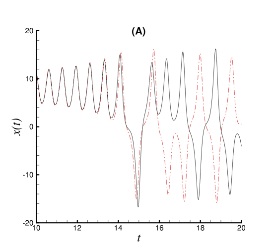
Figure 1: Comparison of numerical results $x(t)$ of Lorenz’s equation by the 4th-order Runge-Kutta’s method when $\sigma=10,R=28,b=-8/3$ and $x(0)=-15.8,y(0)=-17.48,z(0)=35.64$. Solid line: $\tau=10^{-5}$; Dash-dotted line: $\tau=10^{-2}$.

5in

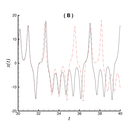
Figure 2: Comparison of numerical results $x(t)$ of Lorenz’s equation by the 4th-order Runge-Kutta’s method when $\sigma=10,R=28,b=-8/3$ and $x(0)=-15.8,y(0)=-17.48,z(0)=35.64$. Solid line: $\tau=10^{-5}$; Dash-dotted line: $\tau=10^{-4}$.

Lorenz [9, 10] and Teixeira et al [18] confirmed such a numerical fact that two computed chaotic results given by either different time-step $\tau$ or different numerical schemes are rather close to each other from the same initial state, until they decouple at a critical time $T_{c}$, as illustrated in Figs. 2 and 2 for comparisons of numerical results of Lorenz’s equation by means of the 4th-order Runge-Kutta’s method with different time-steps in case of $\sigma=10,R=28,b=-8/3$ and $x(0)=-15.8,y(0)=-17.48,z(0)=35.64$. Note that the numerical result given by the time-step $\tau=10^{-2}$ LTU decouples the result given by $\tau=10^{-5}$ LTU at about 14.5 LTU, as shown in Figure 2, and the result given by $\tau=10^{-4}$ LTU decouples the result given by $\tau=10^{-5}$ LTU at about 33.5 LTU, as shown in Figure 2, respectively. Besides, Parker [15] also pointed out that a practical way of judging the accuracy of numerical results of a nonlinear dynamical system is to use two (or more) different routines to integrate the same system: the initial time interval over which the two results agree is then assumed to be accurate and predictable. More precisely speaking, the computed results beyond the critical decoupling time $T_{c}$ are not reliable. Here, it should be emphasized that, up to now, it is even not guaranteed that the computed results in the whole region $0\leq t<T_{c}$ given by two different time-steps $\tau$ or various numerical schemes are convergent or very close to the “exact” solution, especially when the time-steps are very close or the numerical schemes are rather similar. Even so, we have many reasons to assume that the computed chaotic results are reliable in the region $0\leq t<T_{c}$, if we properly choose two (or more ) different time-steps and/or numerical schemes. This is mainly because the computed results in the interval $0\leq t\leq T_{c}$ are “predictable”: one can get nearly the same results by different time-step and/or disparate numerical schemes. In this way, we define a time-scale for the concept “long-term” of a computed chaotic result: $t$ is regarded to be “long-term” if $t>T_{c}$. According to Lorenz [8, 9, 10] and Teixeira et al [18], $T_{c}$ is sensitive to initial condition, time-step and numerical schemes used to compute the two different results of the same nonlinear dynamic system with chaos. For convenience, we call $T_{c}$ the “critical predictable time”. Obviously, $T_{c}$ is dependent upon nonlinear differential equations, time-step and numerical schemes, thus the so-called “long-term” is also a relative concept.

The so-called “critical predictable time” $T_{c}$ can be defined in different ways. According to Teixeira et al [18], a numerical result given by the smallest time-step is assumed to be closest to the exact solution. So, Teixeira et al [18] defined $T_{c}$ by means of the state vector L2 norm error between the result obtained by the smallest time-step and the result by a larger one. This kind of definition includes the error at each time-step and thus is a global one for decoupling. However, decoupling of two curves is essentially a local occurrence. Thus, we give here a local definition of “critical predictable time” $T_{c}$, which is based on geometrical characteristic of decoupling of two curves and thus is straightforward. Mathematically, let $u_{1}(t)$ and $u_{2}(t)$ denote two time series given by different numerical routines for a given dynamical system. The so-called “critical predictable time” $T_{c}$ for $u_{1}(t)$ and $u_{2}(t)$ is determined by the criteria

$$\dot{u}_{1}\;\dot{u}_{2}<-\epsilon,\;\;\;\left|1-\frac{u_{1}}{u_{2}}\right|>\delta,\;\;\;\mbox{at $t=T_{c}$, }$$ (7)

where $\epsilon>0$ and $\delta>0$ are two small constants (we use $\epsilon=1$ and $\delta=5\%$ in this paper). Mathematically, the critical predictable time $T_{c}$ can be interpreted as follows: the influence of truncation error, round-off error and inaccuracy of initial condition on numerical solutions is negligible in the interval $0\leq t\leq T_{c}$, so that the computed result is predictable and thus can be regarded as a reliable solution in this interval. Using the concept of the critical predictable time $T_{c}$, the famous statement that “accurate long-term prediction of chaos is impossible” can be more precisely expressed as that “accurate prediction of chaos beyond the critical predictable time $T_{c}$ is impossible”. Here, $T_{c}$ is regarded as a critical point: computed results beyond the critical predictable time $T_{c}$ are doubtable and unreliable. Thus, the critical predictable time $T_{c}$ provides us a strategy to detect the reliable part from a given numerical result.

As pointed out by Lorenz [9, 10], computational chaos (CC) and computational periodicity (CP) are mainly based on the evaluation of Lyapnunov exponent, which is a long-term property. As mentioned above, any computed results for $t>T_{c}$ are doubtable and unreliable, and thus have no meanings. Unfortunately, most of computed “long-term” solutions are often far beyond the critical predictable time $T_{c}$, and thus all related conclusions or computations based on these “long-term” numerical results, such as computational chaos, computational periodicity, Lyapunov exponent and attractors, are doubtable and unreliable, too. Note that, using the concept of the critical predictable time $T_{c}$, the 3rd figure given by Teixeira et al [18] should be interpreted in such a new way: the critical predictable time $T_{c}$ for three computed results given respectively by $\tau=0.01,0.001$ and $0.0001$ LTU is less than 15 LTU, so all computed results beyond $t>15$ LTU have no meanings, and thus one can not make such a conclusion that “different time-step may not only lead to uncertainty in the predictions after some time, but also lead to fundamentally different regimes of the solution” [18]. In fact, by means of the concept of the critical predictable time, the computational uncertainty of prediction, computational chaos (CC) and computational periodicity (CP) can be avoided completely, as shown in §4 for details.

As suggested by Parker [15], all numerical results should be interpreted properly. The critical predictable time $T_{c}$ can be understood as follows: the influence of truncation error, round-off error and inaccuracy of initial condition on computed chaotic solutions is almost negligible in the time interval $0\leq t\leq T_{c}$. Thus, the so-called critical predictable time $T_{c}$ provides us a scale to investigate chaos in a more precise way. This new concept may greatly deepen and enrich our understanding about chaos, as shown later.

3 Influence of numerical scheme and data inaccuracy on $T_{c}$

Since computed chaotic solutions beyond the critical predictable time $T_{c}$ are unreliable, a numerical result with small $T_{c}$ is almost useless. Thus, it is necessary to obtain reliable chaotic solutions with large enough $T_{c}$.

Without loss of generality, let us consider Lorenz’s equation (1) in case of $\sigma=10,R=28,b=-8/3$ with the exact initial condition $x(0)=-15.8$, $y(0)=-17.48$, $z(0)=35.64$. Using the 4th-order Runge-Kutta’s method with different time increment $\tau=10^{-2}$, $10^{-3}$, $10^{-4}$ and $10^{-5}$ LTU (Lorenz time units), the corresponding critical predictable times $T_{c}$ of computed chaotic results are about 13.7 LTU, 24.5 LTU and 32.6 LTU, respectively, as shown in Figs. 2 and 2. So, by means of traditional numerical methods, the critical predictable time $T_{c}$ of computed chaotic results is often not long enough. Teixeira et al [18] found that, for given numerical scheme, the time of decoupling of numerical chaotic solutions for different time step follows a logarithmic rule as a function of time step. Thus, the time-step should be exponentially small for a give critical predictable time $T_{c}$. Lorenz [10] reported some qualitative influences of numerical schemes (based on truncated Taylor series at a few different orders $M$) on the computed chaotic results, but he did not give a quantitative relationship between the critical predictable time $T_{c}$ and the approximation order $M$. Besides, it is a pity that the influence of round-off error on the time of decoupling of computed chaotic results given by different numerical schemes is neglected, mainly because traditional digital computers use in general the floating-point data in either single or double precision only.

Currently, some advanced symbolic computation software, such as Mathematica and Maple, are widely used. In this paper, the symbolic computation software Mathematica is employed for the first time as a computational tool to investigate the influence of various numerical schemes based on truncated Taylor series (6), round-off error and inaccuracy of initial condition on the critical predictable time $T_{c}$. From the view-point of round-off error, symbolic computation is completely different from evaluating floating-point expressions: the round-off error can be almost neglected or even avoided by means of symbolic computation. For example, by means of symbolic computation, we can have the exact result $1/2+1/3=5/6$. Note that, using numerical computation with double precision representations, one has only the approximate result $1/2+1/3\approx 0.8333333333333333$, whose round-off error is about $10^{-16}$. Besides, using the Mathematica command N[Pi, 800], we can get the approximation $\pi\approx 3.1415926535897932384626433832\cdots$, which is accurate even to 800 decimal places! Using such precise data representation based on symbolic computation software, the round-off error can be almost neglected. Let $K$ denote the number of decimal places of all data used in the symbolic software in this paper. By means of different values of $K$, it is easy to investigate the influence of the round-off error on $T_{c}$, as shown later. Furthermore, by means of the scheme (6), the system of Lorenz equations (1) is approximated by a time-continuous system in each interval $t\in[t_{n},t_{n}+\tau]$ as the truncated $M$th-order Taylor’s expansion. Obviously, the truncation error of this scheme is determined by $M$. Therefore, using symbolic computation and the analytic approach described above, it is convenient to control the magnitude of the truncation-error and the round-off error by means of $M$ and $K$, respectively. Clearly, the larger the values of $M$ and $K$, the smaller the truncation error and round-off error, respectively. Thus, the symbolic computation software provides us a useful tool to investigate the influence of truncation-error, round-off error and inaccuracy of initial conditions on the critical predictable time $T_{c}$.

Without loss of generality, we consider here Lorenz equation (1) in case of $\sigma=10,R=28,b=-8/3$ with the initial condition $x(0)=-15.8,y(0)=-17.48,z(0)=35.64$ and the time step $\tau=10^{-2}$, if not mentioned particularly. Note that the initial condition is assumed to be exact. To investigate the influence of the truncation error on computed chaotic results alone, we set a large enough number of decimal places, i.e. $K=\max\left\{200,2M\right\}$, where $M$ is the order of truncated Taylor series (6) of Lorenz’s equation. In this way, the round-off error is much smaller than the truncation error, and thus is negligible. Since the initial condition is assumed to be exact, there exists the truncation error alone, whose magnitude is determined by $M$, the order of truncated Taylor series (6) of Lorenz equation (1). Using different values of $M$ from $M=4$ to $M=110$, we get different computed results with different truncation errors. Using (7) as the criteria of decoupling of two computed trajectories, it is easy to find the corresponding critical predictable time $T_{c}$ of the numerical result given by the smaller $M$. It is found that the critical predictable time $T_{c}$ is directly proportional to $M$, i.e.

$$T_{c}\approx 3M,$$ (8)

as shown in Figure 3.

5.0in

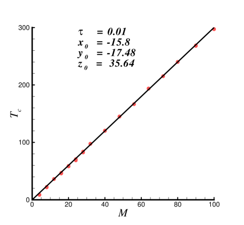
Figure 3: The critical predictable time $T_{c}$ versus the order $M$ of truncated Taylor series (6) in case of $\sigma=10,R=28,b=-8/3$ and $x(0)=-15.8,y(0)=-17.48,z(0)=35.64$ with $K=\max\left\{200,2M\right\}$. Symbols: computed results; Solid line: $T_{c}=3M$.

It is a little more difficult to investigate the influence of the round-off error on chaotic solutions alone, mainly because the round-off error might greatly increase for given $K$ when the order $M$ is too larger than $K$. Note that the previous formula $T_{c}\approx 3M$ (with $K=\max\left\{200,2M\right\}$) gives a time interval $0\leq t\leq T_{c}$ in which the influence of both truncation error and round-off error is negligible, as interpreted before. For example, when $M=32$, the influence of the truncation error is negligible for $t\leq 96$. Thus, without loss of generality, let us consider the case of $M=32$ with different values of $K$ ($K<100$). Comparing the results given by different values of $K$ ($K<100$) with the result obtained by $K=\max\left\{200,2M\right\}$, we get the corresponding critical predictable times $T_{c}$. It is found that, when $K>40$, $T_{c}$ tends to the same value close to 96, respectively. This is mainly because, when $K$ is large enough, the round-off error is much smaller than the truncation error. So, the results for $K>40$ is useless to investigate the influence of the round-off error on $T_{c}$. It is also found that, when $K\leq 16$, the precision of computation is too low relative to the $M$, the order of approximation, so that the round-off error increases greatly. Thus, the results with too small $K$ is also useless. So, only results given by proper values of $K$ are useful. It is found that, for $18\leq K\leq 40$, the computed critical predictable time agree well with the formula

$$T_{c}\approx 2.51K-4.26,$$ (9)

as shown in Figure 4. Furthermore, it is found that, in general, the critical predictable time $T_{c}$ indeed increases linearly with respect to $K$, the number of accurate decimal places of results.

5in

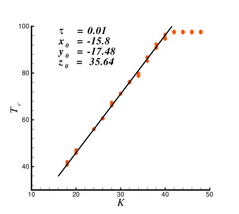
Figure 4: The critical predictable time $T_{c}$ versus $K$ ( the number of accurate decimal places ) in case of $\sigma=10,R=28,b=-8/3$ and $x(0)=-15.8,y(0)=-17.48,z(0)=35.64$ with $M=32$. Symbols: computed results; Solid line: $T_{c}=2.51K-4.26$.

Note that the initial conditions are assumed to be exact in above computations. According to our above investigations, in case of $K=200$ and $M=100$, both of the round-off error and the truncation error are negligible in the interval $0\leq t\leq 300$. This provides us a convenient way to investigate the influence of the inaccuracy of initial conditions on $T_{c}$ alone. To do so, we add a tiny difference $\Delta x_{0}$ into the initial condition $x(0)=-15.8,y(0)=-17.48,z(0)=35.64$ in such a way that

$$x(0)=-15.8+\Delta x_{0},$$

but with the same values of $y(0)$ and $z(0)$. Comparing the results given by different values of $\Delta x_{0}>0$, $M=100$ and $K=200$ with the result given by $\Delta x_{0}=0$, $M=100$ and $K=200$, we obtain the corresponding $T_{c}$ by means of the criteria (7). It is found that, for given different values of $\Delta x_{0}$, the corresponding results of $T_{c}$ agree well with the formula

$$T_{c}\approx-2.5\log_{10}(\Delta x_{0}),$$

as shown in Figure 5. This formula can be rewritten as

$$\Delta x_{0}\approx 10^{-0.4\;T_{c}},$$ (10)

which means that the precision of the initial condition must increase exponentially with respect to a given critical predictable time $T_{c}$. For example, to get a reliable chaotic solution with $T_{c}=200$ LTU, the initial condition must be with the precision $\Delta x_{0}<10^{-80}$. Therefore, we need a rather precise initial condition so as to get a reliable chaotic solution with $T_{c}>200$ LTU. Unfortunately, such precise initial conditions are impossible in practice, as discussed in §5. That is exactly the reason why the “butter-fly effect” exists, as pointed out by Lorenz [8] in 1963. However, the formula (10) might inform us much more than the so-called “butter-fly effect”, as discussed in details in §5.

5in

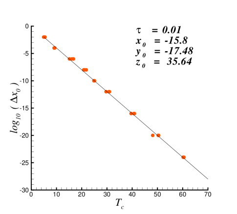
Figure 5: The critical predictable time $T_{c}$ versus the inaccuracy $\Delta x_{0}$ of initial conditions in case of $\sigma=10,R=28,b=-8/3$ and $x(0)=-15.8+\Delta x_{0},y(0)=-17.48,z(0)=35.64$ with $M=100$ and $K=200$. Symbols: computed results; Solid line: $log_{10}(\Delta x_{0})=-0.4T_{c}$.

5in

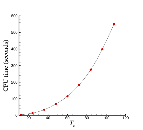
Figure 6: The used CPU time versus $T_{c}$ in case of $\sigma=10,R=28,b=-8/3$ and $x(0)=-15.8,y(0)=-17.48,z(0)=35.64$ with $M=T_{c}/3$ and $K=200$.

Can we get reliable chaotic results with large enough critical predictable time $T_{c}$? Assuming that the initial condition is exact, it is found that $T_{c}\approx 3M$ generally holds in case of $K=\max\left\{200,2M\right\}$. Therefore, $M$ (the order of truncated Taylor series) and $K$ (the number of accurate decimal places) should be increased linearly with respect to the critical predictable time $T_{c}$. So, theoretically speaking, for a given $T_{c}$, one can always find the value of $M$ and $K$ to get a “reliable” chaotic solution in $0\leq t\leq T_{c}$. However, the CPU time increases with respect to $T_{c}$ in a power-law, as shown in Figure 6. Suppose that we would like to get a reliable chaotic solution with $T_{c}=1200$ LTU. According to (8), we should choose $M=400$ so as to get such a reliable chaotic result. In fact, by means of $M=400$ and $K=800$, we indeed obtain this reliable chaotic solution in the interval $0\leq t<1200$ LTU, as shown in Figures 7 and 8. The corresponding result is rather precise: the maximum residual error is only $1.1\times 10^{-481}$. However, more than 461 hours 16 minutes CPU time (more than 19 days) is used by means of a cluster Intel Clovertown Xeon E5310 with 8GB RAM. To the best of our knowledge, such kind of reliable chaotic solution of Lorenz equation in such a long time interval has never been reported. Based on this time-consuming computation, we are quite sure that the solution of Lorenz equation (1) in case of $\sigma=10,R=28$ and $b=-8/3$ is indeed chaotic within the interval $0\leq t<1200$ LTU, as shown in Table 1. However, strictly speaking, it is unknown whether or not the chaotic behavior disappears when $t>1200$ LTU. This is because, based on our current computations, chaotic numerical results beyond $T_{c}$ is unreliable. To answer this question, one had to spend more CPU time to get a reliable chaotic solution with even larger $T_{c}$. Unfortunately, $T_{c}$ is always a finite value, no matter how large it is! And the nonlinearly increased CPU time also indicates the impossibility to get a reliable chaotic solution in an infinite interval $0\leq t<+\infty$. This reveals from the view-point of CPU time that chaos is unpredictable in essence.

5in

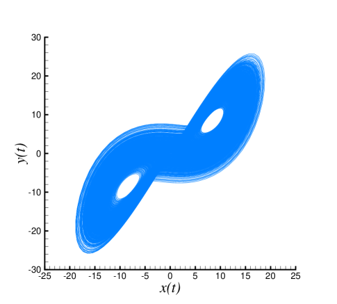
Figure 7: The curve $x(t)-y(t)$ given by the reliable chaotic result with $T_{c}=1200$ LTU by $\tau=0.01,M=400,K=800$ in case of $\sigma=10,R=28,b=-8/3$ and $x(0)=-15.8,y(0)=-17.48,z(0)=35.64$.

5in

Figure 8: The curve $x(t)-z(t)$ given by the reliable chaotic result with $T_{c}=1200$ LTU by $\tau=0.01,M=400,K=800$ in case of $\sigma=10,R=28,b=-8/3$ and $x(0)=-15.8,y(0)=-17.48,z(0)=35.64$.

Table 1: Some reliable numerical results with $T_{c}=1200$ LTU in case of $\sigma=10,R=28,b=-8/3$ by means of $M=400$, $K=800$ and $\tau=0.01$. The detailed data can be downloaded via the website: http://numericaltank.sjtu.edu.cn/.

0	-15.8	-17.48	35.64
50	12.779038299490452	8.825054357006032	36.40092236534542
100	-10.510118721506247	-12.17254281368225	27.476265630374762
150	-1.9674157212680177	-2.5140404626072206	17.233128197642884
200	-6.697233173381982	-11.911020483539128	13.036826414358321
250	3.480010996527037	5.743865139093177	22.424028925951887
300	10.197534991661733	3.906517722362926	35.33742709240441
350	0.009240166388150502	-1.1520585946848019	20.259118270313508
400	-1.8892476498049868	-3.5657880408974663	20.299639635504597
450	2.3442055460290803	2.473910407011588	19.324756580383077
500	-5.30509963157152	-9.425991029211517	12.302184230689779
550	-9.710817000847529	-6.878169205988265	31.67393963382737
600	-0.8635053825976141	0.499057856286716	21.581438144249077
650	-6.249196468824656	-1.3133350412836564	30.3936296733578
700	10.884963668216704	16.32989379246704	22.247458859587212
750	-1.5200586402319973	-0.4164281272461717	21.530357757012936
800	1.3963347154139534	2.40877126758134	14.590441270059282
850	1.580132807298193	2.6273272210193146	12.83939375621528
900	-6.449367823985297	-10.984642417532422	14.647974468278282
950	10.098469202323805	0.4959032511015884	37.72812801085503
1000	13.881997000862393	19.918303160406396	26.901943308376104
1025	-2.831908677750036	-5.127291386139972	10.787422525560384
1050	-6.0495817084397405	-0.5249599507390699	30.805747242725836
1075	-8.445628564097573	-16.91583633884055	8.185099340204886
1100	2.2974592711836634	2.299710874996516	19.617779431769037
1125	-2.0420317363264457	-0.3357510158682992	23.174657463445286
1150	-14.378782424952437	-11.819346602645444	37.319351169225996
1175	-11.794511899005188	-13.181679857519981	29.65720151904728
1200	2.4537546196402595	4.124943247158509	19.349201739150004

4 Avoidance of CC, CP and computational uncertainty of prediction

The uncertainty of prediction of chaos have two reasons. One is computational (or more precisely, mathematical), which is due to nonlinearity of models and the unperfect of numerical schemes and data precision mentioned in §3. The other is physical, which is based on the fundamental physical principles of nature.

In this section, we investigate the computational uncertainty of chaos. In essence, the computational uncertainty of prediction comes from the unpredictability of trajectories, i.e. the decoupling of different trajectories for a “long” time. Using the “critical predictable time” $T_{c}$ and regarding chaotic results reliable only in the interval $0\leq t<T_{c}$, the numerical phenomena such as computational chaos (CC), computational periodicity (CP) and computational uncertainty (CU), can be avoided, as illustrated below.

5.0in

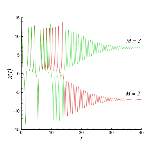
Figure 9: Comparison of $x(t)$ in case of $\sigma=10,R=19,b=-8/3$ with the initial state $x=y=z=5$ by means of $\tau=0.01$ LTU and the $M$th-order scheme (6) based on truncated Taylor series. Red line: $M=2$; Green Line: $M=3$

It is well known that solution of Lorenz’s equation (1) becomes unstable if $R>R_{c}=\sigma(\sigma-b+3)/(\sigma+b-1)$. In case of $\sigma=10$ and $b=-8/3$, we have the critical value $R_{c}=24.7368$. Thus, in case of $\sigma=10,b=-8/3$ and $R=19<R_{c}$ with the initial state $x=y=z=5$, the exact solution should tend to a fixed point. However, it is unknown which fixed point the solution tends to. It is found that the computed result $x(t)$ given by the $M$th-order scheme (6) with $\tau=0.01$ tends to a negative fixed-point for $M=2$, but goes to a positive fixed point for $M=3$, as shown in Figure 9. Thus, at least one of these two different predictions must be wrong. However, based on these two computational results, it is hard to detect which prediction is correct. This kind of computational uncertainty of prediction is similar to those mentioned by Teixeira et al [18]. Note that the critical predictable time $T_{c}$ of these two computed results are only about $T_{c}\approx 9$ LTU, as shown in Figure 9, so that they are reliable only in the interval $0\leq t<9$ LTU. In other words, the two computed results in the interval $t>9$ are unreliable and thus has no meanings. Therefore, based on these two computational results, one can not give any reliable conclusions about the fixed point. To get a reliable prediction about the fixed-point, we had to give a numerical result with large enough $T_{c}$. To do so, we use higher-order schemes (6) based on the truncated Taylor series. As shown in Figure 10, the two computed results given by $M=30$ and $M=40$ with $\tau=0.01$ LTU agree well in the interval $0\leq t\leq 100$ LUT, and both of them give the same numerical fixed-point:

$$x(100)=-6.928204,\;\;y(100)=-6.928204,\;\;z(100)=18.000000.$$

Based on these two reliable numerical results, we are quite sure that the exact solution $x(t)$ of Lorenz equation (1) tends to a negative fixed point in case of $\sigma=10,b=-8/3$ and $R=19<R_{c}$ with the initial state $x=y=z=5$. In this way, the computational uncertainty of prediction mentioned by Teixeira et al [18] and Lorenz [10] can be avoided.

5.0in

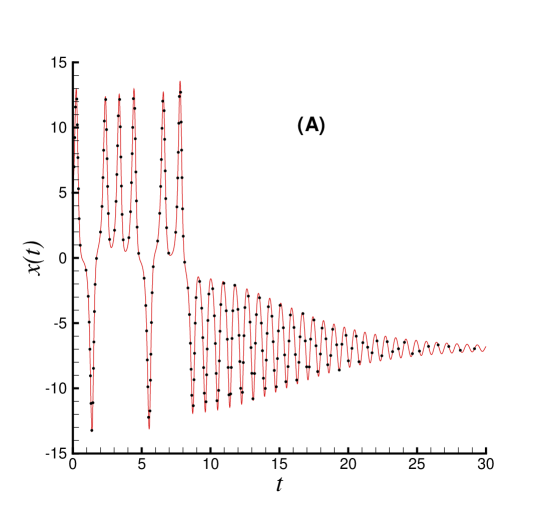
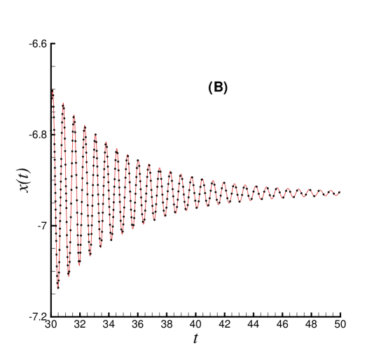
Figure 10: (A) Comparison of $x(t)$ in case of $\sigma=10,R=19,b=-8/3$ with the initial state $x=y=z=5$ by means of $\tau=0.01$ LTU and the $M$th-order scheme (6) based on truncated Taylor series in the interval $0\leq t\leq 30$. Line: $M=30$; Symbols: $M=40$. (B): the same, but in the interval $30\leq t\leq 50$.

5.0in

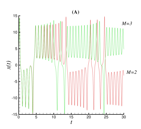
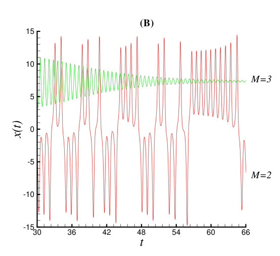
Figure 11: (A) Comparison of $x(t)$ in case of $\sigma=10,R=21.5,b=-8/3$ with the initial state $x=y=z=5$ by means of $\tau=0.01$ LTU and the $M$th-order scheme (6) based on truncated Taylor series in the interval $0\leq t\leq 30$. Red line: $M=2$; Green line: $M=3$. (B): the same, but in the interval $30\leq t\leq 66$.

Similarly, the so-called computational chaos (CC) and computational periodicity (CP) mentioned by Lorenz [9, 10] can be turned away, too. For example, when $\sigma=10,b=-8/3$ and $R=21.5<R_{c}$ with the initial state $x=y=z=5$, it is found that the computed result $x(t)$ given by the $M$th-order scheme (6) based on the truncated Taylor series with $\tau=0.01$ LTU keeps chaotic when $M=2$ but tends to a positive fixed-point when $M=3$, as shown in Figure 11. Since $R=21.5<R_{c}$, the chaotic solution given by $M=2$ is obviously wrong, and the exact solution of $x(t)$ must tend to a fixed point for a large enough time. However, it is not guaranteed whether or not the exact solution of $x(t)$ indeed tends to the positive fixed point. To get a reliable conclusion, computed results with large enough critical predictable time $T_{c}$ are needed. It is found that the computed result given by $M=30$ agrees well with that given by $M=40$ in the interval $0\leq t\leq 100$, as shown in Figure 12. These two results, which are reliable in $0\leq t\leq 100$, clearly indicate that, the solution in case of $\sigma=10,b=-8/3$ and $R=21.5<R_{c}$ with the initial state $x=y=z=5$ is not chaotic, and besides $x(t)$ tends to a negative fixed-point. Thus, both of the two results given by $M=2$ and $M=3$ are wrong: one gives the so-called computational chaos from the result based on $M=2$, and the other a wrong prediction from the result based on $M=3$. In this way, both of computational chaos and computational uncertainty of prediction can be avoided by using reliable results with a large enough critical predictable time $T_{c}$. Similarly, the so-called computational periodicity (CP) can be avoided.

5.0in

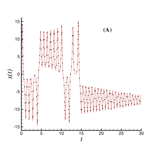
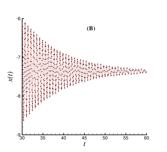
Figure 12: (A) Comparison of $x(t)$ in case of $\sigma=10,R=21.5,b=-8/3$ with the initial state $x=y=z=5$ by means of $\tau=0.01$ LTU and the $M$th-order scheme (6) based on truncated Taylor series in the interval $0\leq t\leq 30$. Line: $M=30$; Symbols: $M=40$. (B): the same, but in the interval $30\leq t\leq 60$.

The above examples illustrate the importance and need of introducing the concept of the critical predictable time $T_{c}$. In this way, computational chaos (CC), computational periodicity (CP), and computational uncertainty of prediction (CUP) of nonlinear dynamic systems can be avoided by using reliable results with a large enough critical predictable time $T_{c}$.

Mathematically, given a critical predictable time $T_{c}$, one can always determine the order $M=T_{c}/3$ of the truncated Taylor series (6), and the number $K=0.4\;T_{c}$ of the accurate decimal places of data by means of (8) and (9) in case of $\sigma=10,R=28,b=-8/3$ with the initial condition $x(0)=-15.8,y(0)=-17.48,z(0)=35.64$, although the needed CPU times might be rather long. So, from pure review-points of mathematics, using the concept of the critical predictable time $T_{c}$, the computational uncertainty of prediction of chaotic dynamical systems can be avoided, as long as we have fast enough computer with large enough memory (RAM).

5 On the origin of prediction uncertainty of chaos

Unfortunately, most nonlinear dynamical systems describe physical phenomena in nature. Thus, results given by these models should have physical meanings. So, it is necessary to investigate the prediction uncertainty of chaos from physical view-points.

The famous Lorenz equation (1) is a macroscopical model for climate prediction on earth: it models a unsteady flow occurring in a layer of fluid of uniform depth $H$ with a constant temperature difference $\Delta T$ between the upper and lower surfaces, and $x(t)$ is proportional to the intensity of convective motion [8]. So, it is reasonable that the influence of physical factors in the level of atom and molecule on the climate is neglected completely in Lorenz equation. On the one hand, for purpose of climate prediction, measured data are unnecessary to be precise in the level of atom and molecule. On the other hand, as output of a macroscopical model, computational results given by Lorenz equation are impossible to be precise in the microcosmis level.

As mentioned in §3, a reliable computational chaotic result with $T_{c}=1200$ LTU is obtained by means of $M=400$ and $K=800$ with the exact initial condition $x(0)=-15.8$, $y(0)=-17.48$, $z(0)=35.64$. Note that $K=800$ corresponds to very precise data. However, according to (8) and (9), it is unnecessary to use such precise data to get a chaotic result with $T_{c}=1200$ LTU. Substituting $T_{c}=1200$ into (8) and (9) give $M=400$ and $K=480$, respectively. Thus, mathematically speaking, the precise data with 480 decimal places must be used in order to get a chaotic result reliable in the interval $0\leq t\leq 1200$ (LTU). This conclusion is obtained with the assumption that the initial condition is exact. Unfortunately, the initial condition is not perfect in practice. It is interesting that, substituting $T_{c}=1200$ into (10) gives $\Delta x_{0}=10^{-480}$. This indicates that the initial condition must be at least with the same accuracy as all computed data used at different time. Therefore, from pure view-points of mathematics, the initial condition (and all computed data) must be with the precision $\Delta x_{0}=10^{-480}$ so as to get a reliable chaotic solution with $T_{c}=1200$ LTU.

First, to show how small the number $10^{-480}$ is, let us compare it with some physical constants. According to NASA’s Wilkinson Microwave Anisotropy Probe (WMAP) project, the age of the universe is estimated to be about $1.373\times 10^{10}$ years, i.e. $T_{u}\approx 4.33\times 10^{17}$ seconds, and its diameter is about 93 billion light years, i.e. $d_{u}\approx 8.8\times 10^{26}$ meter. On the other side, helium is the smallest atom with a radius of 32 picometer, i.e. $r_{a}\approx 3.2\times 10^{-11}$ meter, and the diameter of the nucleus for a proton in light hydrogen is about 1.6 feotometer, i.e. $d_{n}\approx 1.6\times 10^{-15}$ meter. Assume that one object “moves” a distance of radius of helium or a diameter of a proton in light hydrogen since the beginning of the universe, i.e. the Big Bang. Then, the corresponding velocities are $u_{a}=r_{a}/T_{u}\approx 7.39\times 10^{-29}$ (meter/second) and $u_{n}=d_{n}/T_{u}\approx 3.7\times 10^{-33}$ (meter/second), respectively. However, even dividing them by the speed of light $c\approx 3.0\times 10^{9}$ (meter/second) that is assumed to be the largest velocity in nature, we have only the dimensionless velocities $\bar{u}_{a}=r_{a}/(cT_{u})\approx 2.46\times 10^{-38}$ and $\bar{u}_{n}=d_{n}/(cT_{u})\approx 1.23\times 10^{-42}$, respectively. Even so, they are much larger than $10^{-480}$, because both $\bar{u}_{a}\div 10^{-480}=2.46\times 10^{442}$ and $\bar{u}_{n}\div 10^{-480}=1.23\times 10^{438}$ are much greater even than $d_{u}/d_{n}=5.5\times 10^{41}$, the ratio of the diameter of the universe to the diameter of the nucleus for a proton in light hydrogen!

Secondly, according to the Heisenberg uncertainty principle in quantum physics [5], the values of certain pairs of conjugate variables (position and momentum, for instance) cannot both be known with arbitrary precision, and any measurement of the position with accuracy $\Delta\delta$ and the momentum with accuracy $\Delta p$ must satisfy

$$\Delta\delta\;\Delta p\geq\frac{h}{4\pi},$$ (11)

where $h=6.62606896\times 10^{-34}$ [J] [S] is Planck’s constant with the unit [J] of energy (Joule) and the unit [S] of time (Second). Rewriting $\Delta p=m\Delta v$, where $m$ denotes the mass and $v$ the velocity, one has

$$\Delta v\Delta\delta\geq\frac{h}{4\pi m}.$$ (12)

Therefore, the more precisely the velocity $v$ is known, the less precisely the position $\delta$ is known. Because Lorenz equation models the flow of fluid on the earth, the worst measurement of a position is with accuracy $\Delta\delta=d_{E}$, where $d_{E}=1.2745\times 10^{7}$ (meter) is the average diameter of the earth. Then, the most precise measurement of velocity is at most

$$\Delta v\geq\frac{h}{(4\pi d_{E})m}=\frac{4.1372\times 10^{-42}}{m}.$$ (13)

Even if $m$ is regarded as the mass of earth, i.e. $m=5.9742\times 10^{24}$ (kg), the most precise measurement of velocity is at most

$$\Delta v\geq 6.92511\times 10^{-67}(m/s).$$ (14)

Let $\bar{v}$ denote the dimensionless velocity and $U$ the velocity reference, respectively. The above formula gives

$$\Delta\bar{v}\geq\frac{6.92511\times 10^{-67}}{U}.$$

According to the general relativity, light propagates fastest in nature. However, even if the velocity of light is used as the reference velocity, i.e. $U\approx 3.0\times 10^{9}$ (m/s), the most precise measurement of dimensionless velocity on earth is at most

$$\Delta\bar{v}\geq 2.3\times 10^{-76}.$$ (15)

Therefore, it is impossible to measure a dimensionless velocity more precise than the above value. Here, it should be emphasized that the above very tiny number $2.3\times 10^{-76}$ is even much larger than $10^{-480}$: the ratio $(2.3\times 10^{-76})\div 10^{-480}=2.3\times 10^{108}$ is much greater even than $d_{u}/d_{n}=5.5\times 10^{41}$, the ratio of the diameter of the universe to the diameter of the nucleus for a proton in light hydrogen! Therefore, according to the Heisenberg uncertainty principle in quantum physics, it is physically impossible to give an initial condition with the precision $\Delta x_{0}=10^{-480}$, which is however mathematically necessary to get a chaotic result reliable in the interval $0\leq t\leq 1200$ (LTU), as mentioned in §3.

How can we interpret the above interesting result? It seems unavoidable to use nonlinear dynamical models to describe the nature, and besides chaos generally exist in various nonlinear dynamical models. However, as mentioned above, in order to get chaotic results reliable in a long enough time, we need initial condition with precision even higher than the most precise measurement allowed by the Heisenberg uncertainty principle in quantum physics. Note that the precision, which is mathematically necessary for the initial condition and all computed data at different time, is so high that even the quantum-fluctuation becomes a very important physical factor and therefore can not be neglected. Therefore, the famous “butter-flyer effect” of Lorenz equation should be replaced by the so-called “quantum-fluctuation effect”: even the microcosmic physical uncertainty such as quantum-fluctuation may produce a large variations in the long-term macroscopical behavior of a chaotic dynamic system describing natural phenomena.

Thus, although from mathematical points of view we can indeed obtain reliable chaotic solution with $T_{c}>1200$ LTU in case of $\sigma=10,R=28,b=-8/3$ with the exact initial condition $x(0)=-15.8,y(0)=-17.48,z(0)=35.64$ by means of $\tau=0.01$, $M=400$ and $K=480$, unfortunately, this mathematical solution with such a high precision has no physical meanings. It should be emphasized that Lorenz equation is a macroscopical model for climate prediction, and thus microcosmic physical factors such as the quantum-fluctuation are neglected. However, it is mathematically necessary for Lorenz equation to have initial condition with such a high precision that the Heisenberg uncertainty principle in quantum physics must be considered physically. This provides us a “precision paradox of chaos”.

A paradox often brings us much deeper understandings about some thoughts and/or theories. What can such a paradox tell us? It seems that, to avoid this paradox, the following assumptions or view-points should be accepted:

1. Chaos is physically unpredictable. The origin of the unpredictability of chaos comes essentially from the microcosmic uncertainty, which is described by the Heisenberg uncertainty principle in quantum physics;

2. Even macroscopical phenomena might be essentially uncertain, and thus it would be more reliable and more economic to describe them by probability;

3. Most of nonlinear dynamical models, which describe complicated macroscopical phenomena such as chaos and turbulence, do not consider the influence of microcosmic uncertainty, and thus should be modified.

To support the above interprets for the so-called “precision-paradox of chaos”, let us consider the statistic probability of $x(t)$ less than $\mu$, denoted by $P_{x}(\mu)$. The probabilities $P_{x}(\mu)$ obtained by reliable chaotic results with different critical predictable time $T_{c}$ in case of $\sigma=10,R=28,b=-8/3$ with the exact initial condition $x(0)=-15.8,y(0)=-17.48,z(0)=35.64$ by means of $\tau=0.01$ (LTU) are as shown in Figure 13. Note that the probability $P_{x}(\mu)$ given by $T_{c}=75$ LTU agrees well with the probability given by the reliable computational result with $T_{c}=300$ LTU. It indicates that one can obtain a “stable” or “convergent” probability $P_{x}(\mu)$ by means of a reliable result with a proper $T_{c}$ that is unnecessary to be very long. Note that it is much easier to get a reliable chaotic result with $T_{c}=75$ LTU than that with $T_{c}=1200$ LTU! Therefore, it is much cheaper to get a reliable probability $P_{x}(\mu)$ than a reliable time-series $x(t)$ with $T_{c}=1200$ LTU. So, it seems more reliable and especially more “economic” to describe chaotic phenomena by means of probability. This partly supports our above-mentioned interprets about the so-called “precision-paradox of chaos”.

5.0in

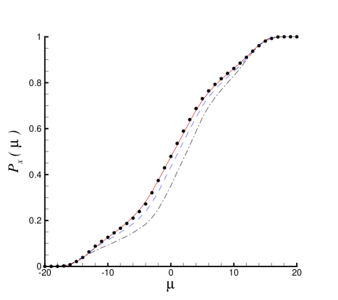
Figure 13: The probability $P_{x}(\mu)$ in case of $\sigma=10,R=28,b=-8/3$ and the exact initial condition $x(0)=-15.8,y(0)=-17.48,z(0)=35.64$ by means of $\tau=0.01$ (LTU) with different $T_{c}$. Symbols: result given by reliable solution with $T_{c}=300$ (LTU); Solid line: result given by reliable solution with $T_{c}=75$ (LTU); Dashed line: result given by reliable solution with $T_{c}=50$ (LTU); Dash-dotted line: result given by reliable solution with $T_{c}=25$ (LTU).

Thus, although the computational uncertainty of chaos can be avoided from the mathematical points of view, it is unavoidable from the physical points of view: the so-called “precision-paradox of chaos” suggests us that the origin of the uncertainty of chaos comes from the Heisenberg uncertainty principle in quantum physics and thus is not avoidable, forever!

6 Discussions

In this paper a new concept, namely the critical predictable time $T_{c}$, is introduced to give a more precise description of computed chaotic solutions of nonlinear differential equations: computed chaotic solutions are regarded to be reliable only when $0<t\leq T_{c}$. This provides us a method or strategy to detect the reliable result from a given computed solution. Besides, it provides us a time scale for the so-called “long-term”: $t$ is regarded to be long-term as long as $t>T_{c}$. It is also suggested that numerical results beyond the critical predictable time $T_{c}$ are unpredictable, and thus all related conclusions based on computed chaotic results beyond the critical predictable time $T_{c}$ are unreliable and doubtable. In this way, the numerical phenomena such as computational chaos (CC), computational periodicity (CP) and computational prediction uncertainty, which are mainly based on long-term properties of computed results, can be avoided, as shown in §4. By means of this concept, the famous conclusion “accurate long-term prediction of chaos is impossible” should be replaced by a more precise conclusion that “accurate prediction of chaos beyond the critical predictable time $T_{c}$ is impossible”.

For a nonlinear dynamic system with chaotic behavior, one had to solve it by at least two different computation schemes so as to get the critical predictable time $T_{c}$. Certainly, it is better to use more different computation schemes to investigate the reliability of computed results with chaos: the more, the better. So, the reliability of chaotic solutions is a relative concept: it is dependent on not only nonlinear differential equations but also the accuracy of initial guess, time-step and computation schemes. Without knowing the exact solution, such kind of reliable solutions within the critical predictable time $T_{c}$ might be the best in practice: they are at least predictable, i.e. different computation schemes lead to very close results. Note that even the definition (7) of the critical predictable time is dependent upon the two constants $\delta$ and $\epsilon$. Fortunately, the same qualitative conclusions can be obtained even by different (but reasonable) values of $\delta$ and $\epsilon$. So, all of our conclusions mentioned in this paper have general meanings.

On the one hand, the so-called critical predictable time $T_{c}$ provides us a scale to investigate chaos more precisely. On the other hand, the symbolic computation software (such as Mathematica) provide us a convenient way to investigate the influence of truncation-error, round-off error, and inaccuracy of initial guess on the critical predictable time $T_{c}$. It is found that $T_{c}$ is directly proportional to $M$, the order of the truncated Taylor series (6), and $K$, the number of decimal places of all computed data. Besides, the precision of initial conditions must increase exponentially as $T_{c}$ enlarges. For example, in case of $\sigma=10,R=28,b=-8/3$ with the initial condition $x(0)=-15.8,y(0)=-17.48,z(0)=35.64$, we obtain a reliable chaotic result with $T_{c}=1200$ LTU by means of $\tau=0.01$ (LTU), $M=400$ and $K=800$. Such a reliable chaotic solution in so long time is reported for the first time. Mathematically, given a critical predictable time $T_{c}$, we can always get a reliable chaotic result in the interval $0\leq t\leq T_{c}$ by means of a high-performance computer with large enough memory (RAM) and fast enough CPU, although the needed CPU time might be rather long. Therefore, in essence, the computational uncertainty of prediction for chaos can be avoided, if only from the mathematical points of view.

However, the precision of initial condition and computed data at each time-step needed for a large $T_{c}$ (such as $T_{c}=1200$ LTU) is mathematically so high that such precise data is physical impossible due to Heisenberg uncertainty principle in quantum physics. Note that the precision, which is mathematically necessary for the initial condition and all computed data at different time, is so high that even the quantum-fluctuation becomes a very important physical factor and therefore can not be neglected. But, as a macroscopical model for climate prediction on earth, Lorenz equation completely neglects the influence of physical factors in the level of atom and molecule on the climate. This provides us the so-called “precision-paradox of chaos”, which implies that the prediction uncertainty of chaos is physically unavoidable and besides even the macroscopical phenomena might be essentially stochastic and thus should be described by probability more economically.

Many nonlinear evaluation equations for macroscopical phenomena, such as Lorenz equation for climate prediction and Navier-Stokes equation for turbulent viscous flows, completely neglect the influence of physical factors in the level of atom and molecule. However, the so-called “precision paradox of chaos” suggests that this might be wrong: the influence of physical factors in the level of atom and molecule should be considered for complicated nonlinear dynamic systems. It is well-known that turbulent flows are much more complicated than chaos. So, one should be very careful to apply numerical schemes to investigate turbulent flows. Currently, the DNS (direct numerical simulation) is frequently used in computational fluid dynamics (CFD) to simulate turbulence flows [6, 13, 16, 14, 12]. However, it is a pity that the mathematical sensitivity of DNS results for turbulent flows to the inaccuracy of initial conditions, round-off error and truncation error has not been studied systematically, mainly because the DNS is rather time-consuming. Without a method or strategy to detect the reliability of a given DNS result, we has many reasons to assume that something without physical meanings (similar to computational periodicity and computational chaos mentioned by Lorenz [9, 10]) might be contained in the so-called DNS “solutions” for turbulence, and thus conclusions based on such kind of unreliable computed results might be doubtable. More importantly, all models for turbulent flows completely neglect the influence of microcosmic factors in physics. And this might be one of the reasons why there is no a satisfactory model to describe all turbulent flows precisely.

Note that the concept of the critical predictable time $T_{c}$ is not new: it is rather similar to the so-called “critical decoupling time” mentioned by Teixeira et al [18]. However, this concept has never been obtained enough recognition. In this paper, we shaw the importance of such kind of concept for the reliability of computed chaotic results, and also for the avoidance of computational prediction uncertainty, computational chaos (CC) and computational periodicity (CP). More importantly, the concept of critical predictable time $T_{c}$ greatly deepens and enriches our understanding about chaos, not only mathematically but also physically.

Nonlinear dynamical systems describing chaos or turbulence might be much more complicated than we thought: we should feel awe to them. It is the time for us to consider seriously the reliability of a mass of computed chaotic or turbulent results reported every day!

Acknowledgement The author would like to express his sincere thanks to Dr. L.S. Yao, Dr. D. Hughes, and Dr. J. Teixeira for providing some valuable references. Thanks to the anonymous referees for their valuable comments.

References

- [1] Ashwin, P. 2003. Synchronization from chaos. Nature, 42, 384-385.
- [2] Cloutman, L.D. 1996. A note on the stability and accuracy of finite difference approximations to differential equations. Report No. UCRL-ID-125549, Lawrence Livermore National Laboratory.
- [3] Cloutman, L.D. 1998. Chaos and instabilities in finite difference approximations to nonlinear differential equations. Report No. UCRL-ID-131333, Lawrence Livermore National Laboratory.
- [4] Hanski, I., Turchin, P., Korplmäki, E. and Henttonen, H. 1993. Population oscillations of boreal rodents: regulation by mustelid predators leads to chaos. Nature, 364, 232-235.
- [5] Heisenberg, W. 1927. Über den anschaulichen Inhalt der quantentheoretischen Kinematik und Mechanik. Zeitschrift für Physik, 43, 172-198.
- [6] Le, H., Moin, P. and Kim, J. 1997. Direct numerical simulation of turbulent flow over a backward-facing step, J. of Fluid Mechanics, 330, 349-374.
- [7] Li, T.Y. and Yorke, J.A. 1975. Period three implies chaos. Amer. Math. Monthly, 10, 985-992.
- [8] Lorenz, E.N. 1963. Deterministic nonperiodic flow. J. Atmos. Sci., 20, 130-141.
- [9] Lorenz, E.N. 1989. Computational Chaos: a prelude to computational instability. Physica D, 35, 299-317.
- [10] Lorenz, E.N. 2006. Computational periodicity as observed in a simple system. Tellus A, 58, 549-557.
- [11] Malescio, G. 2005. Predicting with unpredictability. Nature, 1073, 434.
- [12] Mart n, M.P., Taylor, E.M., Wu, M. and Weirs, V.G. 2006. A bandwidth-optimized WENO scheme for the effective direct numerical simulation of compressible turbulence. J. Computational Phys., 220 (1), 270-289.
- [13] Moin, P. and Mahesh, K. 1998. Direct numerical simulation: a tool in turbulence research. Annual Review of Fluid Mechanics, 30, 539-578.
- [14] Moser, R.D., Kim, J. and Mansour, N.N. 1999. Direct numerical simulation of turbulent channel flow up to Re = 590. Phys. Fluids, 11, 943.
- [15] Parker, T.S. and Chua, L.O. 1989. Practical Numerical Algorithms for Chaotic Systems. Springer-Verlag, New York.
- [16] Scardovelli, R. and Zaleski, S. 1999. Direct numerical simulation of free-surface and interfacial flow. Annual Review of Fluid Mechanics, 31, 567-603.
- [17] Stewart, I. 2000. The Lorenz attractor exists. Nature, 406, 948-949.
- [18] Teixeira, J., Reynolds, C.A. and Judd, K. 2007. Time step sensitivity of nonlinear atmospheric models: numerical convergence, truncation error growth, and ensemble design. J. Atmos. Sci., 64, 175-189.
- [19] Teixeira, J., Reynolds, C.A. and Judd, K. 2008. Reply to Yao and Hughes’ comments. J. Atmos. Sci., 65, 683-684.
- [20] Yao, L.S. and Hughes, D. 2008a. Comment on “Computational periodicity as observed in a simple system” By Edward N. Lorenz (2006). Tellus A, 60, 803-805.
- [21] Yao, L.S. and Hughes, D. 20008b. Comments on “Time step sensitivity of nonlinear atmospheric models: numerical convergence, truncation error growth, and ensemble design”. J. Atmos. Sci., 65, 681-682.