Nous proposons une nouvelle méthode pour estimer les ruptures du rythme cardiaque dans les bandes parasympathiques et orthosympathiques basée sur la transformée en ondelettes dans le domaine complexe et l’étude des ruptures des moments des modules de ces transformées en ondelettes. Nous observons des ruptures dans la distribution pour les deux bandes de fréquence. We propose a new method for estimating the change-points of heart rate in the orthosympathetic and parasympathetic bands, based on the wavelet transform in the complex domain and the study of the change-points in the moments of the modulus of these wavelet transforms. We observe change-points in the distribution for both bands. Detection of Change–Points in the Spectral Density Bertrand, Teyssière, Boudet, Chamoux Detection of Change–Points in the Spectral Density.
With Applications to ECG Data Pierre R. Bertrand, Gilles Teyssière, Gil Boudet, Alain Chamoux

1 Introduction

ECG signal analysis has a long story after the implementation of the ambulatory monitoring by Holter at the beginning of the fifties. Recent measurement methods, due to the size reduction of the measurement devices, see Chamoux (1984), allow us to record ECG data for healthy people over a long period of time: long distance (marathon) runners, individuals daily (24 hours) records, etc. We then obtain large datasets that allow us to characterize the variations of the heartbeat rate in the two components of the nervous autonomous system: the parasympathetic and the orthosympathetic ones.

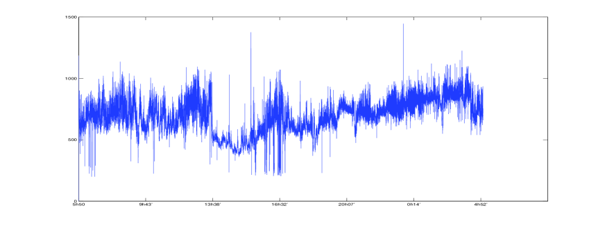
Figure 1: RR interval for a healthy subject during a period of 24 hours

The data studied in this paper have been recorded the 29^th of January 2008, at the Clermont-Ferrand University Hospital (CHU) by G. Boudet. Unlike Boudet et al. (2004) and Cottin et al (2006), these data are not recorded in the framework of a laboratory experiment, but during the real life of the individual under investigation.

We have daily datasets, over 100,000 observations, and in the near future we will have data over several days, i.e., over that sample size. We are measuring the interval between two RR peaks, i.e., if we denote by $(t_{i})_{i=1,\dots,N}$, the sequence of peak times measured with a precision of 1.E-03 second, we consider the series $X(t_{i})=\Big{(}t_{i}-t_{i-1}\Big{)}$ measured in seconds. Several indicators are related to heartbeat data. The most popular is the instantaneous average frequency, i.e., $X(t_{i})^{-1}$, which is displayed by runners watches. This quantity is informative on daily activity of observed individual: sleeping and waking up times, physical activity, e.g., sport, manual work, but does not summarize all relevant information. Note that heartbeat data display large variations, clustering, etc, as only individuals with serious disease display a regular heart rate.

Cardiologists are interested in the study of this signal in two frequency bands: the orthosympathetic and parasympathetic bands, i.e., the frequency bands $(0.04\,Hz,\,0.15\,Hz)$ and $(0.15\,Hz,\,0.5\,Hz)$ respectively. The definition of these bands is the outcome of research works, see e.g., Task force of the European Society of Cardiology and the North American Society of Pacing and Electrophysiology (1996), and is based on the fact that the energy contained inside these bands would be a relevant indicator on the level of the stress of an individual.

Indeed, for the heart rate, the parasympathetic system is often compared to the brake while the orthosympathetic system would be a nice accelerator; see e.g. Goldberger (2001). At rest there is a permanent braking effect on the heart rate. Any solicitation of the cardiovascular system, any activity initially produces a reduction of parasympathetic brake followed by a gradual involvement of the sympathetic system. These mechanisms are very interesting to watch in many diseases including heart failure, but also rhythm disorders that may fall under one or other of these two effects, monitoring the therapeutic effect of several Medicines including some psychotropic. In the field of physiology such data are crucial for measuring the level of vigilance and particularly the risk of falling asleep while driving a vehicle, the level of stress induced by physical activity or level of perceived stress, which can be considered as a criterion of overtraining in sport.

Fractals models have been used in cardiology after the works by Ivanov et al. (1999), who applied the multifractal spectrum analysis advocated by Frisch (1996), for modeling RR series and classifying individuals according to this multifractal spectrum, as this spectrum discriminates between individuals who experienced hearth trouble, and those who did not. However, this tool has some shortcomings as it requires huge samples common in turbulence analysis, and is then inappropriate for studying phenomena occurring at a resolution lower than the daily time interval, such as the variations of the parasympathetic and orthosympathetic systems inside the day.

Wavelets based methods have been used in biostatistics by Diab et al. (2007) for uterine EMG signal analysis. However, they consider that the process studied is homogeneous, and used these methods as a classification tool. Another significant difference is the fact that they use discrete wavelet decomposition, i.e., a frequency decomposition on a dyadic wavelet basis, the choice for the frequency bands is made without reference to a biological phenomenon. In our case, the choice for the frequency band is justified by biological considerations, and we fit the wavelets inside these bands.

This is why the continuous analysis of both systems and their quantification is a particularly promising research area. So, the example in Figures 4, 5, 6 shows at the observation 28,220 i.e., 13h40’50”, a simultaneous variation of both systems.

2 Mathematical formulation

For biological reasons, the heart rate is within the interval $[20,250]$ bpm (beats per minute), i.e., $X(t)$ belongs to the RR interval $60/250s.<X(t)<60/20s.$. This leads to modeling by stationary or locally stationary processes. We wish to decompose this signal in a sequence of homogeneous intervals having the same mean and/or variance. We make the assumption that the series is Gaussian, and then find the optimal segmentation of the process using the same approach as in Lavielle and Teyssière (2006) or Lavielle and Moulines (2000).

We assume that the signal is the sum of a piecewise constant function and a Gaussian process, centered and locally stationary. We then have the following representation:

$$X(t)=\mu(t)+\int_{I\!\!R}e^{it\xi}f^{1/2}(t,\xi)\,dW(\xi),\quad\mbox{for all}\quad t\in R,$$ (1)

where

• $\xi\mapsto f(t,\xi)$ is an even and positive function, called spectral density piecewise constant, i.e., there exists a partition

  $\tau_{1},\dots,\tau_{K}$ such that $f(t,\xi)=f_{k}(\xi)$ for $t\in[\tau_{i},\tau_{i+1}[$

• the function $t\mapsto\mu(t)$ is also piecewise constant for another partition $\widetilde{\tau}_{1},\dots,\widetilde{\tau}_{L}$ with $\mu(t)=\mu_{\ell}$ if $t\in[\widetilde{\tau}_{\ell},\,\widetilde{\tau}_{\ell+1}[$

The wavelet coefficient associated with $\psi$ is

$$W_{\psi}(b)=\int_{I\!\!R}\psi(t-b)X(t)\,dt\hskip 28.45274pt\mathrm{unit\;in}\;second^{2}.$$ (2)

In Bardet and Bertrand (2007) or Bardet et al. (2008), one can find a theoretical study of the wavelet coefficient for stationary (or with stationary increment) centered Gaussian processes, i.e., for $X$ given by (1) with $\mu(t)=0$. This approach can be generalized to locally stationary Gaussian processes, this will be detailed in a forthcoming paper.

According to recommendations of Task force of the European Soc. Cardiology and the North American Soc. of Pacing and Electrophysiology (1996), we use the following notations:

• $[\omega_{1},\omega_{2}]=(0.04\,Hz,\,0.15\,Hz)$ denotes the orthosympathetic frequency band,

• $[\omega_{2},\omega_{3}]=(0.15\,Hz,\,0.5\,Hz)$ denotes the parasympathetic band

The energy associated with each of these frequency bands and localized around the time $b$, is measured by the modulus of the complex wavelet coefficients $|W_{i}(b)|^{2}$ for $i=1,2$, with

$$b\longmapsto W_{i}(b) = \int_{I\!\!R}\psi_{i}(t-b)\,X(t)\,dt,\quad i=1,2.$$

In this work, these wavelets coefficients are computed at each second, i.e., the difference between two consecutive values for $b$ is equal to 1 second.

How to choose the wavelets $\psi_{1}$ and $\psi_{2}$ ?

In the idealistic case, one would use two filters $\psi_{1}$ and $\psi_{2}$ with compact support, the Fourier transforms of which have support inside the orthosympathetic and parasympathetic bands.

Unfortunately, it does not exist a non null function $\psi$ with compact time domain support and compact frequency support, see for instance Mallat (1998) Th 2.6 p.34. Therefore, the best we can do is to choose between a filter with a compact frequency support and a filter with a compact time domain support. The first choice is well suited for stationary models, see Bardet and Bertrand (2007). But, in this work, we are interested by locally stationary models, thus our specifications are a filter with compact time domain support as a Daubechies wavelet. The price to pay for the compactness of the time domain support is the loss in the compactness of the frequency support. However, the frequency support is "almost compact" in the following sense:

Definition 2.1 ($\rho$ pseudo support)

Let $0<\rho<1$, be a map $g\in L^{2}(I\!\!R)$ that admits the compact interval $I$ as a $\rho$ pseudo support if $\,\displaystyle\frac{\int_{I}|g(t)|^{2}\,dt}{\int_{I\!\!R}|g(t)|^{2}\,dt}=\rho.$

Fourier transform of Daubechies wavelet have a reasonably small $\rho$ pseudo support with a ratio $\rho$ close to $1$. Moreover, the larger the number of the Daubechies wavelet is, the closer to $1$ the ratio $\rho$ is; see the example below with the Daubechies wavelet D6.

By scaling and modulation, one can adjust the pseudo support inside a specified frequency band as stated by the following proposition

Proposition 2.1

Let $\psi$ be a filter with compact support $[L_{1},L_{2}]$ and a frequency $\rho$ pseudo support $[\Lambda_{1},\Lambda_{2}]$, for any frequencies band $[\omega_{1},\omega_{2}]$, the map $\,\displaystyle\psi_{1}(t)=\mu\times e^{i\eta t}\,\psi(\lambda t)$ with

$$\mu>0,\qquad\lambda=\frac{\omega_{2}-\omega_{1}}{\Lambda_{2}-\Lambda_{1}} \mathrm{and} \eta=\frac{\omega_{1}+\omega_{2}}{2}-(\omega_{2}-\omega_{1})\frac{\Lambda_{2}+\Lambda_{1}}{\Lambda_{2}-\Lambda_{1}}$$

has a $\rho$ pseudo support $[\omega_{1},\omega_{2}]$ and a time domain support $\displaystyle\left[\frac{\Lambda_{2}-\Lambda_{1}}{\omega_{2}-\omega_{1}}L_{1},\frac{\Lambda_{2}-\Lambda_{1}}{\omega_{2}-\omega_{1}}L_{2}\right]$.

Proof. Since $\displaystyle\widehat{\psi_{1}}(\xi)=\mu\times\widehat{\psi}\left(\frac{\xi-\eta}{\lambda}\right)$, one can deduce $\;\displaystyle\rho\;pseudo\,supp\,\psi_{1}=\eta+\lambda\times\rho\;pseudo\;supp\,\psi\;$ and then the proposition.  

Different choices for the wavelets $\psi_{1}$ and $\psi_{2}$

From Proposition 2.1, one can deduce the different possible choices of the filters $\psi_{1}$ and $\psi_{2}$

• Daubechies wavelet D6: In this case, we have $\Lambda_{1}=0.08$, $\Lambda_{2}=1.75$, $\rho=0.9999$ and one can set

  $$\psi_{1}(t)=\mu\times e^{i\eta_{1}t}\,D_{6}(\lambda_{1}t)\quad\mathrm{and}\quad\displaystyle\psi_{2}(t)=\mu\times e^{i\eta_{2}t}\,D_{6}(\lambda_{2}t)$$

  $$\mathrm{with}\quad\eta_{1}=-0.0255,\lambda_{1}=0.0659,\eta_{2}=-0.0585,\;\mathrm{and}\;\lambda_{2}=0.2096.$$

  The length of the time support are $\left|Supp\,\psi_{1}\right|$ and $\left|Supp\,\psi_{2}\right|$. One can see on Fig. 2 (a) that the Fourier transforms $\widehat{\psi}_{1}(x)$ and $\widehat{\psi}_{2}(x)$ have almost disjoint supports.

  $$\lambda_{1}=\frac{\omega_{2}-\omega_{1}}{\Lambda_{2}-\Lambda_{1}} \mathrm{and} \eta_{1}=\frac{\omega_{1}+\omega_{2}}{2}-(\omega_{2}-\omega_{1})\frac{\Lambda_{2}+\Lambda_{1}}{\Lambda_{2}-\Lambda_{1}}$$

  $$\lambda_{2}=\frac{\omega_{3}-\omega_{2}}{\Lambda_{2}-\Lambda_{1}} \mathrm{and} \eta_{2}=\frac{\omega_{2}+\omega_{3}}{2}-(\omega_{3}-\omega_{2})\frac{\Lambda_{2}+\Lambda_{1}}{\Lambda_{2}-\Lambda_{1}}$$

  $$\left|Supp\,\psi_{1}\right|=\frac{\Lambda_{2}-\Lambda_{1}}{\omega_{2}-\omega_{1}}\times\left|Supp\,D_{6}\right| \mathrm{and} \left|Supp\,\psi_{2}\right|=\frac{\Lambda_{2}-\Lambda_{1}}{\omega_{3}-\omega_{2}}\times\left|Supp\,D_{6}\right|$$

• Gabor wavelet: For computational reasons, we will use the Gabor wavelet defined as

  $$\psi(t)=e^{i\eta t}g(t),\quad g(t)=\frac{1}{(\sigma^{2}\pi)^{1/4}}\,e^{-\frac{t^{2}}{2\sigma^{2}}}$$ (3)

  see, e.g., Mallat (1998). This wavelet has the same time and frequency $\rho$ pseudo support $[-L,L]=[-3.5,3.5]$ with $\rho=0.9995$. In the spectral domain, we have

  $$\widehat{\psi}(t)=\hat{g}(\xi-\eta),\quad\hat{g}(\xi)=(4\pi\sigma^{2})^{1/4}e^{\frac{-\sigma^{2}\xi^{2}}{2}}$$ (4)

  We fit the Gabor wavelet inside the orthosympathetic or the parasympathetic frequency bands by using Prop. 2.1 or direct calculations. One obtains the two Gabor wavelets defined by (3) with the following choice for the parameters:

  $$\eta_{1}=\frac{\omega_{1}+\omega_{2}}{2} \mathrm{and} \sigma_{1}=\frac{2L}{\omega_{2}-\omega_{1}}$$

  $$\eta_{2}=\frac{\omega_{2}+\omega_{3}}{2} \mathrm{and} \sigma_{2}=\frac{2L}{\omega_{3}-\omega_{2}}$$

  $$\mathrm{moreover}\qquad\left|\rho\,pseudo\,Supp\,\psi_{1}\right|=\frac{4L^{2}}{\omega_{2}-\omega_{1}} \mathrm{and} \left|\rho\,pseudo\,Supp\,\psi_{2}\right|=\frac{4L^{2}}{\omega_{3}-\omega_{2}}\quad\mathrm{with}\;\rho=0.9995$$

  One can see on Fig. 2 that the Fourier transforms $\widehat{\psi}_{1}(x)$ and $\widehat{\psi}_{2}(x)$ still have almost disjoint supports.

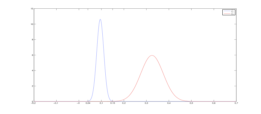
Figure 2: The Fourier transforms $\widehat{\psi}_{1}(x)$ (left) and $\widehat{\psi}_{2}(x)$ (right)

Using the Gabor wavelet is more efficient in terms of computing time, as it is at least 8 times faster. Figure 3 below displays the Gabor wavelets coefficients in the orthosympathetic and parasympathetic bands respectively for the sample plotted in Figure 1.

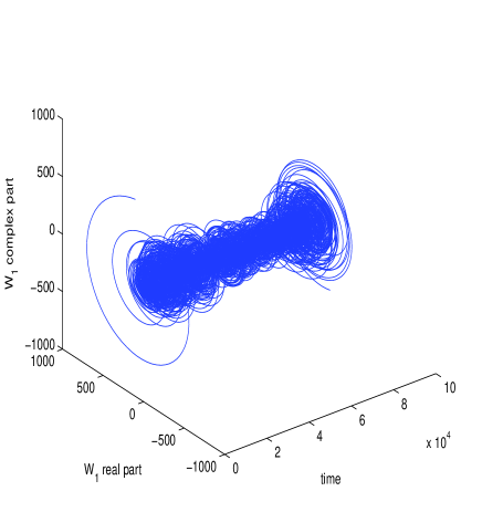
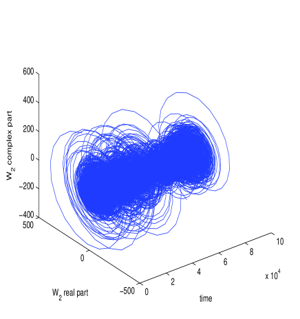
Figure 3: The wavelet coefficients in the orthosympathetic band (left) and in the parasympathetic band (right) of the same healthy subject during a period of 24 hours

3 Segmentation analysis

We assume that the process $\{X_{t}\}$ is abruptly changing and is characterized by a parameter $\theta\in\Theta$ that remains constant between two changes. We use this assumption to define our contrast function $J(\boldsymbol{\tau},\boldsymbol{X})$. Let $K$ be some integer and let $\boldsymbol{\tau}=\{\tau_{1},\tau_{2},\ldots,\tau_{K-1}\}$ be an ordered sequence of integers satisfying $0<\tau_{1}<\tau_{2}<\ldots<\tau_{K-1}<n$.

For the detection of changes in the mean and variance of a sequence of random variables, i.e., a change in distribution, we use the following contrast function, based on a Gaussian log–likelihood function:

$$J_{n}(\boldsymbol{\tau},\boldsymbol{X})=\frac{1}{n}\sum_{k=1}^{K}\frac{\|X_{\tau_{k}}-\bar{X}_{\tau_{k}}\|^{2}}{\hat{\sigma}_{k}^{2}}+n_{k}\log(\hat{\sigma}_{k}^{2}).$$ (5)

where $n_{k}=\tau_{k}-\tau_{k-1}$ is the length of segment $k$, $\hat{\sigma}_{k}^{2}$ is the empirical variance computed on that segment $k$, $\hat{\sigma}_{k}^{2}=n_{k}^{-1}\sum_{i=\tau_{k-1}+1}^{\tau_{k}}(X_{i}-\bar{X})^{2}$, and $\bar{X}$ is the empirical mean of $X_{1},\ldots,X_{n}$.

In fact, we minimize a penalized version of this contrast function, the penalty parameter being selected in an adaptive way so that the obtained segmentation does not depend too much on the penalty parameter; see also Birgé and Massart (2007) for another choice for the penalty parameter. Although this method has been devised for Gaussian processes, it empirically provides relevant results for non-Gaussian processes, e.g., financial time series, see Lavielle and Teyssière (2006) for further details.

3.1 Orthosympathetic band

For that frequency band, we obtain the following segmentation:

$$\boldsymbol{\tau}=\{28220,33366,71048\},$$

i.e., 13h40’50”, 15h06’36”, 1h34’38”.

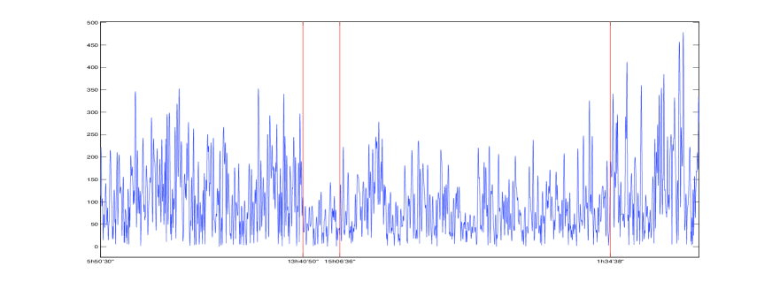
Figure 4: Segmentation in the mean and variance (change in the distribution) of the modulus of the wavelet coefficients in the orthosympathetic band

3.2 Parasympathetic band

For that frequency band, we obtain the following segmentation:

$$\boldsymbol{\tau}=\{11620,21912,28054,31540,36022,40172,52622,70550\},$$

i.e., 9h04’10”, 11h45’42”, 13h38’04”, 14h36’10”, 15h50’22”, 17h00’02”, 20h27’32”, 1h26’40”.

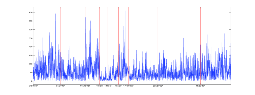
Figure 5: Segmentation in the mean and variance (change in the distribution) of the modulus of the wavelet coefficients in the parasympathetic band

4 Conclusion

The example illustrated by Figures 4, 5 and 6 shows at around $t=28,220$ a simultaneous variation of both systems. But, one can also observe change-points in the orthosympathetic and parasympathetic bands occurring at different times. In the future, we will study the existence of a possible causality or sequentiality between these change–points in different bands.

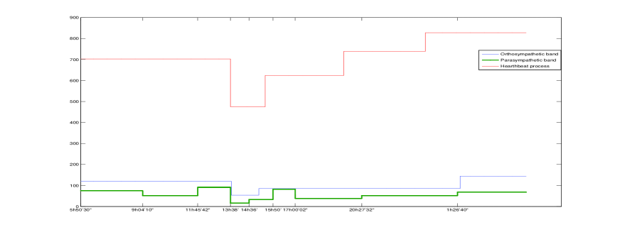
Figure 6: Mean of the modulus if the wavelets coefficients for the orthosympathetic and parasympathetic bands, and of the RR process $X(t)$

References

- (1) Bardet, J.M. and Bertrand, P.R. (2007). Identification of the multiscale fractional Brownian motion with biomechanical applications. J. Time Ser. Anal. 28, 1–52.
- (2) Bardet, J.M., Bertrand, P.R. and Billat, V. (2008). Estimation non-paramétrique de la densité spectrale d’un processus gaussien observé à des instants aléatoires. Pub. ISUP 52, 123–138.
- (3) Birgé, L. and Massart, P. (2007). Minimal penalties for Gaussian model selection. Probab. Theory Related Fields 138, 33–73.
- (4) Boudet, G., Albuisson, E., Bedu, M. and Chamoux, A. (2004). Heart rate running speed relationships during exhaustive bouts in the laboratory. Can. J. Appl. Physiol. 29(6), 731–742.
- (5) Chamoux, A. (1984). Le système Holter en pratique. Médecine du Sport 58, 43-273, 54–284.
- (6) Cottin, F., Leprêtre, PM., Lopes, P., Papelier, Y., Médigue, C. and Billat V. (2006). Assessment of ventilatory thresholds from heart rate variability in well-trained subjects during cycling, Int. J. Sports Med. 27, 959–967.
- (7) Diab, M.O., Marque, C. and Khalil, M.A. (2007). Classification for uterine EMG Signals: Comparison between AR model and statistical classification method. Int. J. Computational Cognition 5, 8–14,
- (8) Frisch, U. (1996). Turbulence. Cambridge University Press.
- (9) Goldberger, A.L. (2001). Heartbeats, hormones and health : is variability the spice of life ? Am. J. Crit. Care Med. 163, 1289–1290.
- (10) Ivanov, P.C., Amaral, L.A.N., Goldberger, A.L., Havlin, S., Rosenblum, M., Struzik, Z, and Stanley, H.E. (1999). Multifractality in human heartbeat dynamics. Nature 399, 461–465.
- (11) Lavielle, M. and Moulines, E. (2000). Least-squares estimation of an unknown number of shifts in a time series. J. of Time Series Anal. 21, 33–59.
- (12) Lavielle, M. and Teyssière, G. (2006). Detection of multiple change-points in multivariate time series. Lithuanian Math. J. 46, 287–306. [Détection de ruptures multiples dans des séries temporelles multivariées.] (Translation in French) Liet. Mat. Rink. 46, 351–376.
- (13) Mallat, S. (1998). A wavelet tour of signal processing. Academic Press.
- (14) Task force of the European Soc. Cardiology and the North American Society of Pacing and Electrophysiology (1996). Heart rate variability. Standards of measurement, physiological interpretation, and clinical use. Circulation 93, 1043–1065.