Abstract

We numerically investigate the features of typical orbits occurring in the Oort cloud ($r\approx 50-150$ kAU) in the low-acceleration regime of the MOdified Newtonian Dynamics (MOND). We fully take into account the so-called External Field Effect (EFE) because the solar system is embedded in the Milky Way. In the framework of MOND this does matter since the gravitational acceleration of Galactic origin felt by the solar system is of the same order of magnitude of the characteristic MOND acceleration scale $A_{0}\approx 10^{-10}$ m s^-2. We use three different forms of the MOND interpolating function $\mu(x)$, two different values for the Galactic field at the Sun’s location and different initial conditions corresponding to plausible Keplerian ellipses in the Oort cloud. We find that MOND produces highly distorted trajectories with respect to the Newtonian case, especially for very eccentric orbits. It turns out that the shape of the MOND orbits strongly depend on the initial conditions. For particular initial state vectors, the MOND paths in the ecliptic plane get shrunk extending over much smaller spatial regions than in the Newtonian case, and experience high frequency variations over one Keplerian orbital period. Ecliptic orbits with different initial conditions and nearly polar orbits are quite different getting distorted as well, but they occupy more extended spatial regions. These facts may have consequences on the composition and the dynamical history of the Oort cloud which are difficult to predict in detail; certainly, the MOND picture of the Oort region is quite different from the Newtonian one exhibiting no regularities.

Keywords: gravitation $-$ celestial mechanics $-$ Oort cloud

1 Introduction

In many astrophysical systems like, e.g., spiral galaxies and clusters of galaxies a discrepancy between the observed kinematics of their exterior parts and the predicted one on the basis of the Newtonian dynamics and the matter detected from the emitted electromagnetic radiation (visible stars and gas clouds) was present since the pioneering studies, in recent times, by Bosma [1] and Rubin and coworkers [2] on spiral galaxies. More precisely, such an effect shows up in the galactic velocity rotation curves whose typical pattern after a few kpc from the center differs from the Keplerian $1/\sqrt{r}$ fall-off expected from the usual dynamics applied to the electromagnetically-observed matter.

As a possible solution of this puzzle, the existence of non-baryonic, weakly-interacting Cold Dark (in the sense that its existence is indirectly inferred only from its gravitational action, not from emitted electromagnetic radiation) Matter (CDM) was proposed to reconcile the predictions with the observations [3] in the framework of the standard gravitational physics.

Oppositely, it was postulated that the Newtonian laws of gravitation may have to be modified on certain acceleration scales to correctly account for the observed anomalous kinematics of such astrophysical systems without resorting to still undetected exotic forms of matter. One of the most phenomenologically successful modification of the inverse-square Newtonian law, mainly with respect to spiral galaxies, is the MOdified Newtonian Dynamics (MOND) [4, 5, 6] which postulates that for systems experiencing total gravitational accelerations $A<A_{0}$, with [7]

$$A_{0}=(1.2\pm 0.27)\times 10^{-10}\ {\rm m\ s}^{-2},$$ (1)

the overall gravitational acceleration felt gets modified according to

$$\boldsymbol{A}\rightarrow\boldsymbol{A}_{\rm MOND}=-\frac{\sqrt{A_{0}GM}}{r}\boldsymbol{\hat{r}}.$$ (2)

More generally, it holds

$$A=\frac{A_{\rm Newton}}{\mu(x)},\ x\equiv\frac{A}{A_{0}};$$ (3)

$\mu(x)\rightarrow 1$ for $x\gg 1$, i.e. for large accelerations (with respect to $A_{0}$), while $\mu(x)\rightarrow x$ yielding eq. (2) for $x\ll 1$, i.e. for small accelerations. The most widely used forms for the interpolating function $\mu$ are [8, 9]

$$\mu_{1}(x) = \frac{x}{1+x},$$ (4)

$$\mu_{2}(x) = \frac{x}{(1+x^{2})^{1/2}}.$$ (5)

Such forms, and also others, as we will see later, can be reduced to the following high-acceleration limit ($x\gg 1$)

$$\mu\approx 1-k_{0}x^{-\alpha}.$$ (6)

Indeed, eq. (4) corresponds to $k_{0}=1$, $\alpha=1$, while eq. (5) corresponds to $k_{0}=1/2$ and $\alpha=2$. It recently turned out that the simpler form of eq. (4) yields better results in fitting the terminal velocity curve of the Milky Way, the rotation curve of the standard external galaxy NGC 3198 [8, 10, 11] and of a sample of 17 high surface brightness, early-type disc galaxies [12]. Eq. (3) strictly holds for co-planar, spherically and axially symmetric isolated mass distributions [13]; otherwise, for generic mass densities the full modified (non-relativistic) Poisson equation [9]

$$\boldsymbol{\nabla}\boldsymbol{\cdot}\left[\mu\left(\frac{|\boldsymbol{\nabla}U|}{A_{0}}\right)\boldsymbol{\nabla}U\right]=4\pi G\rho,$$ (7)

where $U$ is the gravitational potential, $G$ is the Newtonian constant of gravitation and $\rho$ is the matter density generating $U$, must be used.

Attempts to yield a physical foundation to MOND, especially in terms of a relativistic covariant theory, can be be found in, e.g., [14, 15, 16]; for recent reviews of various aspects of the MOND paradigm, see [17, 18, 19].

After setting the theoretical background which we will use in the rest of the paper, we will explore the strong MONDian regime in the remote ($r=50-150$ kAU) periphery of the solar system, where the Oort cloud [20], populated by a huge number of small bodies moving along very eccentric and inclined to the ecliptic orbits, is supposed to exist; for preliminary investigations on such a topic, see [4, 21]. In particular, we will numerically investigate the modifications that MOND would induce on the Newtonian orbits of a test particle moving in such a region. We will also have to consider the subtle External Field Effect (EFE) which, in MOND, takes into account the influence of the Galactic field in the dynamics of the bodies of the solar system giving rise, in the regions in which $x\ll 1$, to a total gravitational acceleration quite different from the scheme consisting of the Newtonian one plus some perturbative correction(s) to it.

For other works on MOND in the inner regions of the solar system, see Ref. [4, 22, 23, 24, 25, 26, 27, 28, 32, 33].

2 The External Field Effect in MOND

In the framework of MOND, the internal dynamics of a gravitating system s embedded in a larger one S is affected by the external background field $\boldsymbol{E}$ of S even if it is constant and uniform, thus implying a violation of the Strong Equivalence Principle: it is the so-called External Field Effect (EFE). In the case of the solar system, $E$ would be $A_{\rm cen}\approx 10^{-10}$ m s^-2 because of its motion through the Milky Way [4, 9, 21].

Clarifying EFE’s concrete effects on the orbital dynamics of s is not an easy task also because of some possible misunderstandings due to the intrinsic difficulty of the subject. The existence in the inner regions of the solar system of its simplest form, i.e. a constant and uniform vector field $\boldsymbol{E}$ added to the standard Newtonian monopole with $E\approx 10^{-10}$ m s^-2, has been ruled out in Ref. [29] by comparing analytical calculation with the estimated corrections $\Delta\dot{\varpi}$ to the standard perihelion precessions of some planets determined with the EPM ephemerides by E.V. Pitjeva (RAS, IAA) [30]; it turned out that the upper bound on an anomalous acceleration with the characteristics of $\boldsymbol{E}$ is of the order of $10^{-14}$ m s^-2. Such a result has been recently confirmed by W.M. Folkner [31], although in a different context, with a modified version of the latest DE ephemerides by NASA JPL including a constant and uniform extra-acceleration with which he fitted long observational data records. Milgrom in Ref. [32] has put forth a different form for the planetary EFE yielding an additional quadrupolar extra-acceleration which mimics the action of distant mass; some consequences have been investigated in Ref. [33].

Moving to the remote periphery of the solar system, which is our present target, let us define the following quantities

$$\eta \doteq \frac{A_{\rm cen}}{A_{0}}\gtrsim 1,$$ (8)

$$r_{t} \doteq \sqrt{\frac{GM}{A_{0}}}=6.833\ {\rm kAU},$$ (9)

$$L \doteq \frac{x}{\mu}\left(\frac{{{d}}{\mu}}{{{d}}{x}}\right),$$ (10)

$$\mu_{g} \doteq \mu(\eta),$$ (11)

$$L_{g} \doteq L(\eta).$$ (12)

In the weak acceleration regime, for

$$r\gg{r_{t}}\eta^{-1/2},$$ (13)

which is fully satisfied in the Oort cloud, the action of EFE is different, so that the total barycentric acceleration felt by an Oort comet is [9, 32]

$$\boldsymbol{A}=-\frac{GM}{\mu_{g}(1+L_{g})^{1/2}}\left(\frac{x^{2}}{1+L_{g}}+y^{2}+z^{2}\right)^{-\frac{3}{2}}\left(\begin{array}[]{c}\frac{x}{1+L_{g}}\\ y\\ z\\ \end{array}\right).$$ (14)

It must be stressed that, contrary to what it could be thought at first sight, eq. (14) is not a small correction to the Newtonian monopole $\boldsymbol{A}_{\rm Newton}=-(GM/r^{2})\boldsymbol{\hat{r}}$ to be tackled with the usual perturbative techniques like, e.g., the Gauss equations for the variation of the elements. Indeed, eq. (14) must be treated as a whole because it is the total gravitational pull felt by a body in the weak acceleration regime according to MOND; it fully embeds EFE which cannot be disentangled. The only consistent alternative to the MONDian acceleration of eq. (14) is the standard Newtonian term. It may be interesting to show, from a purely phenomenological point of view, that applying eq. (14) to the major bodies of the solar system in its planetary regions yields absurd results. Indeed, by considering, e.g., the Earth, the discrepancy between eq. (14) and the standard Newtonian monopole turns out to be of the order of $2-8\times 10^{-4}$ m s^-2 which corresponds to an enormous shift of up to $1\times 10^{10}$ m in the heliocentric radial distance of our planet.

Note that, since the ecliptic longitude and latitude of the Galactic Center are about $\lambda_{\rm GC}\approx 180$ deg, $\beta_{\rm GC}\approx-6$ deg [33], EFE is directed along the $X$ axis of the ICRF, i.e. the barycentric frame in which the motion of solar system’s objects are usually studied. Concerning $L$, we have

$$\mu_{1}=\frac{x}{1+x} \rightarrow L_{1}=\frac{1}{1+x},$$ (15)

$$\mu_{2}=\frac{x}{(1+x^{2})^{1/2}} \rightarrow L_{2}=\frac{1}{1+x^{2}},$$ (16)

$$\mu_{3/2}=\frac{x}{(1+x^{3/2})^{2/3}} \rightarrow L_{3/2}=\frac{1}{1+x^{3/2}}.$$ (17)

The value of $\eta$ depends on the Galactic field at the solar system’s location which can be obtained from its centrifugal acceleration

$$A_{\rm cen}=\frac{V^{2}}{R},$$ (18)

where $V$ is the speed of the Local Standard of Rest (LSR) and $R=8.5$ kpc is the Galactocentric distance. The standard IAU value for the LSR speed is $V=220$ km s^-1 [34], but recent determinations obtained with the Very Long Baseline Array and the Japanese VLBI Exploration of Radio Astronomy project yield a higher value: $V=254\pm 16$ km s^-1 [35]. Thus, $\eta$ ranges from 1.5 to 2.3.

3 Orbits of Oort comets in MOND

3.1 Ecliptic orbits

We will, now, consider an Oort comet whose Newtonian orbit covers the entire extension of the Oort cloud. It has semimajor axis $a=100$ kAU and eccentricity $e=0.5$, so that its perihelion is 50 kAU and its aphelion is 150 kAU; for the sake of simplicity, we will assume it lies in the ecliptic plane. Its Newtonian orbital period is $P_{\rm b}=31.6$ Myr. We will, first, use $\mu_{3/2}$. The value $\eta=2.0$, corresponding to $V=254\ {\rm km\ s^{-1}}$, yields

$$\mu_{g} = 0.82$$ (19)

$$L_{g} = 0.25$$ (20)

Figure 1 depicts the numerically integrated Newtonian (dashed blue line) and MONDian (dash-dotted red line) orbits for the same initial conditions. The integration has been performed backward in time over one (Keplerian) orbital period.

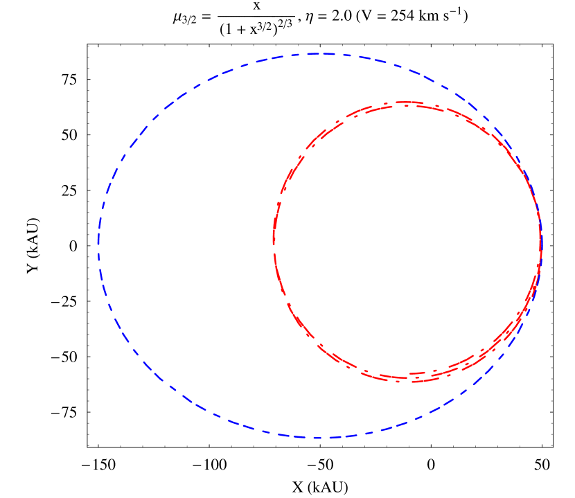
Figure 1: Numerically integrated orbits of an Oort comet with $a=100$ kAU, $e=0.5$, $P_{\rm b}=31.6$ Myr. Dashed blue line: Newton. Dash-dotted red line: MOND with $\mu_{3/2}$, $\eta=2.0$ ($V=254$ km s^-1). The initial conditions are $x_{0}=a(1-e),y_{0}=z_{0}=0,\dot{x}_{0}=0,\dot{y}_{0}=na\sqrt{\frac{1+e}{1-e}},\dot{z}_{0}=0$. The time span of the integration is $-P_{\rm b}\leq t\leq 0$.

In Figure 2 we show the case $\eta=1.5\ (V=220\ {\rm km\ s^{-1}})$ yielding

$$\mu_{g} = 0.75$$ (21)

$$L_{g} = 0.34.$$ (22)

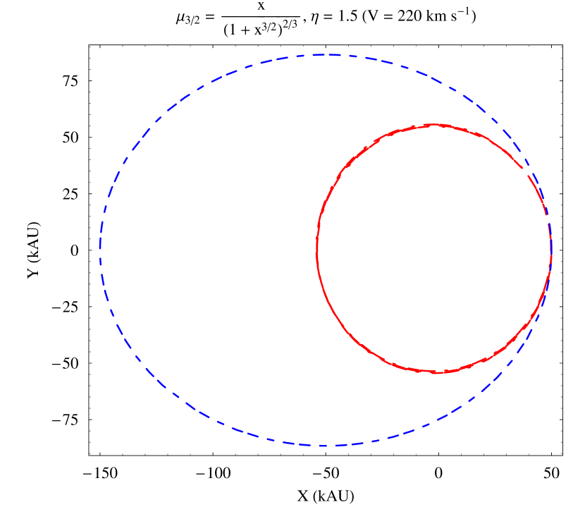
Figure 2: Numerically integrated orbits of an Oort comet with $a=100$ kAU, $e=0.5$, $P_{\rm b}=31.6$ Myr. Dashed blue line: Newton. Dash-dotted red line: MOND with $\mu_{3/2}$, $\eta=1.5$ ($V=220$ km s^-1). The initial conditions are $x_{0}=a(1-e),y_{0}=z_{0}=0,\dot{x}_{0}=0,\dot{y}_{0}=na\sqrt{\frac{1+e}{1-e}},\dot{z}_{0}=0$. The time span of the integration is $-P_{\rm b}\leq t\leq 0$.

The MOND trajectories are not closed and the points of minimum and maximum distances from the Sun do not coincide with the Newtonian ones. In general, they do not show a regular pattern. Moreover, the MOND paths are much less spatially extended that the Newtonian ones; the overall shrinking of the orbit is more marked for the standard value of the LSR circular speed (Figure 2). Finally, the MOND trajectories experience high frequency variations during one (Keplerian) orbital period. Such effects are particularly notable for highly elliptical Newtonian orbits, as shown by Figure 3- Figure 4 for $e=0.9$ and $-P_{\rm b}\leq t\leq 0$. In the Newtonian case, their perihelia are at 10 kAU, while the aphelia lie at 190 kAU, so that the condition of eq. (13) is still well fulfilled.

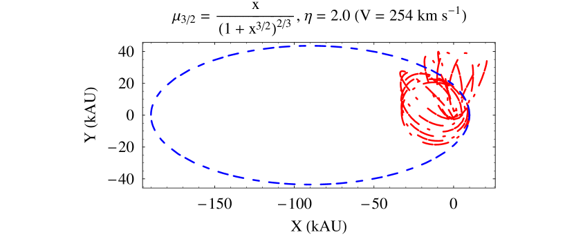
Figure 3: Numerically integrated orbits of an Oort comet with $a=100$ kAU, $e=0.9$, $P_{\rm b}=31.6$ Myr. Dashed blue line: Newton. Dash-dotted red line: MOND with $\mu_{3/2}$, $\eta=2.0$ ($V=254$ km s^-1). The initial conditions are $x_{0}=a(1-e),y_{0}=z_{0}=0,\dot{x}_{0}=0,\dot{y}_{0}=na\sqrt{\frac{1+e}{1-e}},\dot{z}_{0}=0$. The time span of the integration is $-P_{\rm b}\leq t\leq 0$.

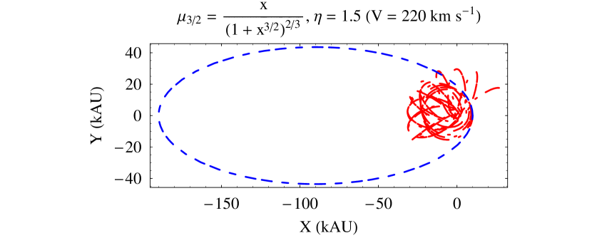
Figure 4: Numerically integrated orbits of an Oort comet with $a=100$ kAU, $e=0.9$, $P_{\rm b}=31.6$ Myr. Dashed blue line: Newton. Dash-dotted red line: MOND with $\mu_{3/2}$, $\eta=1.5$ ($V=220$ km s^-1). The initial conditions are $x_{0}=a(1-e),y_{0}=z_{0}=0,\dot{x}_{0}=0,\dot{y}_{0}=na\sqrt{\frac{1+e}{1-e}},\dot{z}_{0}=0$. The time span of the integration is $-P_{\rm b}\leq t\leq 0$.

The MOND orbits resemble involved clews comprised within 60 kAU $\times$ 60 kAU.

At this point, it must be noted that in Figure 1-Figure 4 we used the state vector at the perihelion as initial conditions for the numerical integrations. We have to check if the behavior described is somewhat related to the peculiar initial conditions chosen. To this aim, in Figure 5-Figure 6 we consider paths starting at the (Newtonian) aphelion for $e=0.5$,

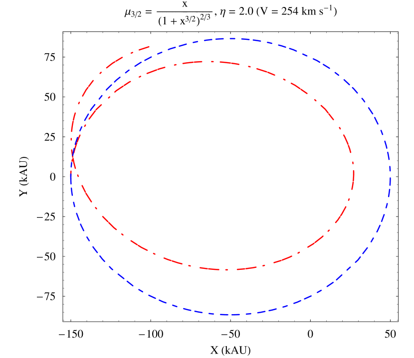
Figure 5: Numerically integrated orbits of an Oort comet with $a=100$ kAU, $e=0.5$, $P_{\rm b}=31.6$ Myr. Dashed blue line: Newton. Dash-dotted red line: MOND with $\mu_{3/2}$, $\eta=2.0$ ($V=254$ km s^-1). The initial conditions are $x_{0}=-a(1+e),y_{0}=z_{0}=0,\dot{x}_{0}=0,\dot{y}_{0}=-na\sqrt{\frac{1-e}{1+e}},\dot{z}_{0}=0$. The time span of the integration is $-P_{\rm b}\leq t\leq 0$.

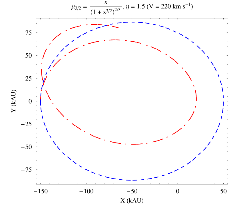
Figure 6: Numerically integrated orbits of an Oort comet with $a=100$ kAU, $e=0.5$, $P_{\rm b}=31.6$ Myr. Dashed blue line: Newton. Dash-dotted red line: MOND with $\mu_{3/2}$, $\eta=1.5$ ($V=220$ km s^-1). The initial conditions are $x_{0}=-a(1+e),y_{0}=z_{0}=0,\dot{x}_{0}=0,\dot{y}_{0}=-na\sqrt{\frac{1-e}{1+e}},\dot{z}_{0}=0$. The time span of the integration is $-P_{\rm b}\leq t\leq 0$.

while the case $e=0.9$ is depicted in Figure 7-Figure 8. Also in this cases we integrated the equations of motion backward in time over one (Keplerian) orbital period $P_{\rm b}$.

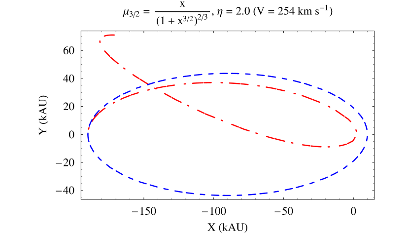
Figure 7: Numerically integrated orbits of an Oort comet with $a=100$ kAU, $e=0.9$, $P_{\rm b}=31.6$ Myr. Dashed blue line: Newton. Dash-dotted red line: MOND with $\mu_{3/2}$, $\eta=2.0$ ($V=254$ km s^-1). The initial conditions are $x_{0}=-a(1+e),y_{0}=z_{0}=0,\dot{x}_{0}=0,\dot{y}_{0}=-na\sqrt{\frac{1-e}{1+e}},\dot{z}_{0}=0$. The time span of the integration is $-P_{\rm b}\leq t\leq 0$.

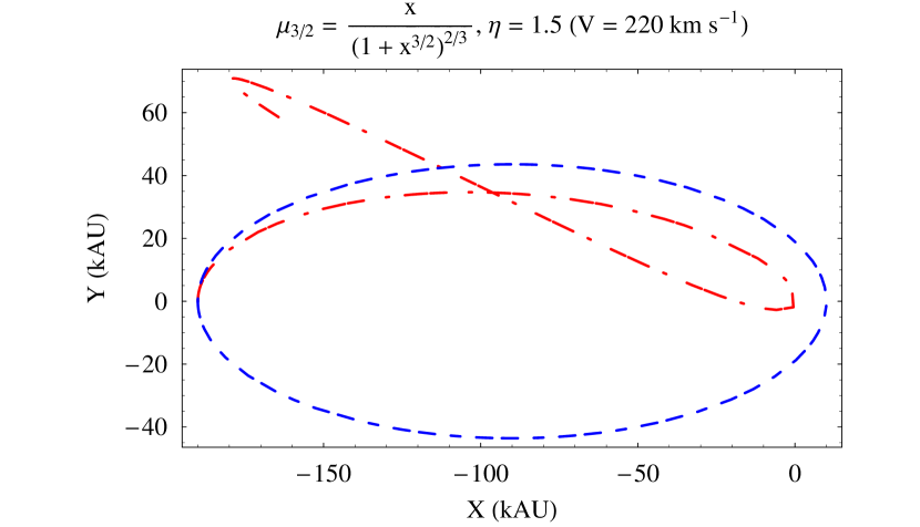
Figure 8: Numerically integrated orbits of an Oort comet with $a=100$ kAU, $e=0.9$, $P_{\rm b}=31.6$ Myr. Dashed blue line: Newton. Dash-dotted red line: MOND with $\mu_{3/2}$, $\eta=1.5$ ($V=220$ km s^-1). The initial conditions are $x_{0}=-a(1+e),y_{0}=z_{0}=0,\dot{x}_{0}=0,\dot{y}_{0}=-na\sqrt{\frac{1-e}{1+e}},\dot{z}_{0}=0$. The time span of the integration is $-P_{\rm b}\leq t\leq 0$.

It can be noted that the MOND trajectories starting at the (Newtonian) aphelion are quite different with respect to those starting at the (Newtonian) perihelion depicted before. Again, they are not close and no regular patterns occur. In this case, the areas swept by the MOND paths are larger than in the previous case, and they occupy a large part of the Newtonian ones. For $e=0.9$ the MOND orbits approximately lie within 180 kAU $\times$ 60 kAU.

The case for $\mu_{2}$ is rather similar, so that we will not depict the related figures for saving space.

Let us, now, examine the case $\mu_{1}$. In Figure 9 we show the trajectory due to it of the Oort comet with $e=0.5$ over $P_{\rm b}$ for $\eta=2.0$ which implies

$$\mu_{g} = 0.67$$ (23)

$$L_{g} = 0.33.$$ (24)

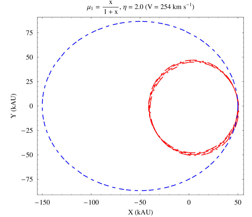
Figure 9: Numerically integrated orbits of an Oort comet with $a=100$ kAU, $e=0.5$, $P_{\rm b}=31.6$ Myr. Dashed blue line: Newton. Dash-dotted red line: MOND with $\mu_{1}$, $\eta=2.0$ ($V=254$ km s^-1). The initial conditions are $x_{0}=a(1-e),y_{0}=z_{0}=0,\dot{x}_{0}=0,\dot{y}_{0}=na\sqrt{\frac{1+e}{1-e}},\dot{z}_{0}=0$. The time span of the integration is $-P_{\rm b}\leq t\leq 0$.

The case $\eta=1.5$, yielding

$$\mu_{g} = 0.60$$ (25)

$$L_{g} = 0.39,$$ (26)

is shown in Figure 10 for $-P_{\rm b}\leq t\leq 0$.

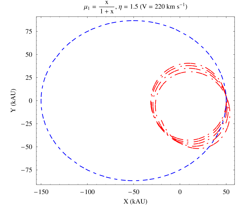
Figure 10: Numerically integrated orbits of an Oort comet with $a=100$ kAU, $e=0.5$, $P_{\rm b}=31.6$ Myr. Continuous blue line: Newton. Dash-dotted red line: MOND with $\mu_{1}$, $\eta=1.5$ ($V=220$ km s^-1). The initial conditions are $x_{0}=a(1-e),y_{0}=z_{0}=0,\dot{x}_{0}=0,\dot{y}_{0}=na\sqrt{\frac{1+e}{1-e}},\dot{z}_{0}=0$. The time span of the integration is $-P_{\rm b}\leq t\leq 0$.

The case of highly elliptic orbits ($e=0.9$) is more intricate, as shown by Figure 11 and Figure 12.

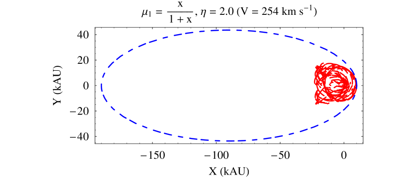
Figure 11: Numerically integrated orbits of an Oort comet with $a=100$ kAU, $e=0.9$, $P_{\rm b}=31.6$ Myr. Dashed blue line: Newton. Dash-dotted red line: MOND with $\mu_{1}$, $\eta=2.0$ ($V=254$ km s^-1). The initial conditions are $x_{0}=a(1-e),y_{0}=z_{0}=0,\dot{x}_{0}=0,\dot{y}_{0}=na\sqrt{\frac{1+e}{1-e}},\dot{z}_{0}=0$. The time span of the integration is $-P_{\rm b}\leq t\leq 0$.

Figure 12: Numerically integrated orbits of an Oort comet with $a=100$ kAU, $e=0.9$, $P_{\rm b}=31.6$ Myr. Dashed blue line: Newton. Dash-dotted red line: MOND with $\mu_{1}$, $\eta=1.5$ ($V=220$ km s^-1). The initial conditions are $x_{0}=a(1-e),y_{0}=z_{0}=0,\dot{x}_{0}=0,\dot{y}_{0}=na\sqrt{\frac{1+e}{1-e}},\dot{z}_{0}=0$. The time span of the integration is $-P_{\rm b}\leq t\leq 0$.

Indeed, the MOND paths resemble confuse clews confined within small spatial regions shifted with respect to the $\mu_{3/2}$ case.

Also the trajectories of Figure 9-Figure 12 start from the (Newtonian) perihelia. If, instead, we choose the (Newtonian) aphelia quite different paths occur also for this form of $\mu$. Figure 13-Figure 16 show them.

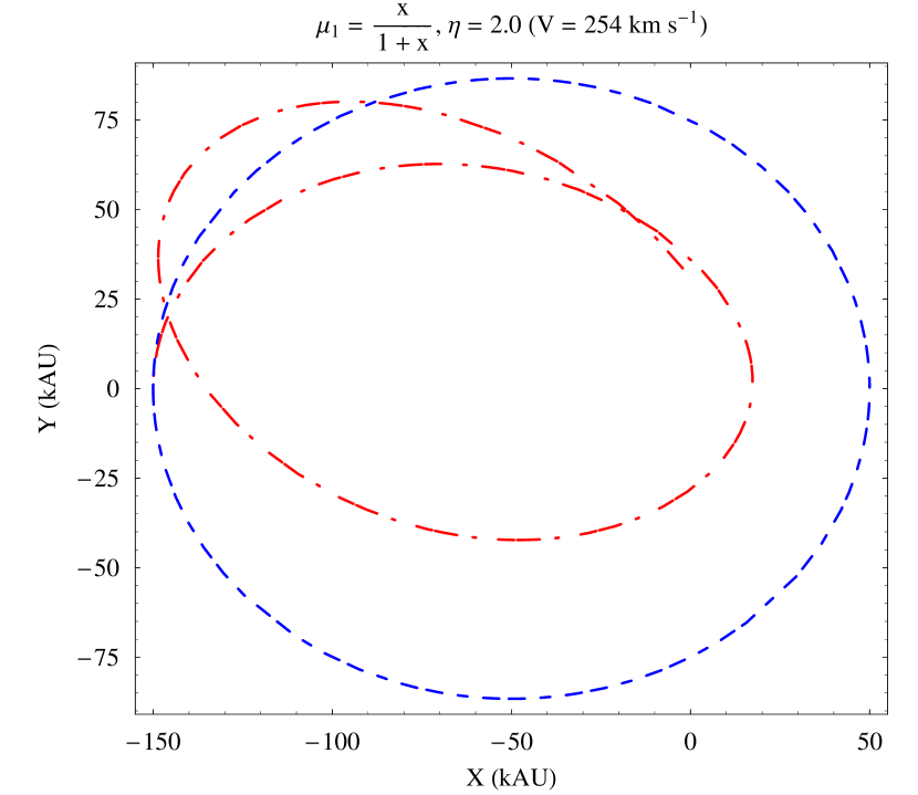
Figure 13: Numerically integrated orbits of an Oort comet with $a=100$ kAU, $e=0.5$, $P_{\rm b}=31.6$ Myr. Dashed blue line: Newton. Dash-dotted red line: MOND with $\mu_{1}$, $\eta=2.0$ ($V=254$ km s^-1). The initial conditions are $x_{0}=-a(1+e),y_{0}=z_{0}=0,\dot{x}_{0}=0,\dot{y}_{0}=-na\sqrt{\frac{1-e}{1+e}},\dot{z}_{0}=0$. The time span of the integration is $-P_{\rm b}\leq t\leq 0$.

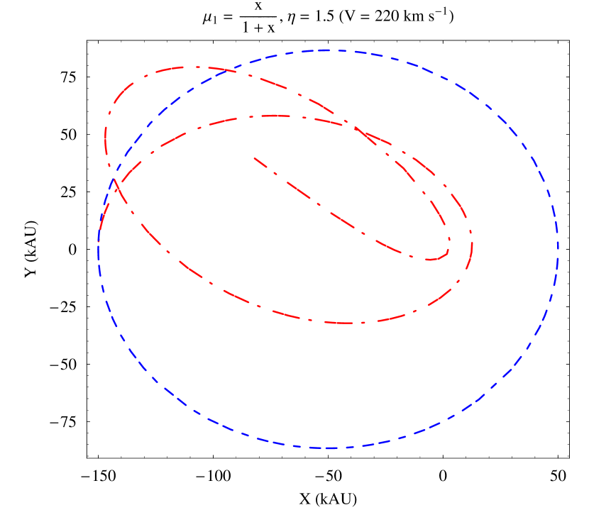
Figure 14: Numerically integrated orbits of an Oort comet with $a=100$ kAU, $e=0.5$, $P_{\rm b}=31.6$ Myr. Continuous blue line: Newton. Dash-dotted red line: MOND with $\mu_{1}$, $\eta=1.5$ ($V=220$ km s^-1). The initial conditions are $x_{0}=-a(1+e),y_{0}=z_{0}=0,\dot{x}_{0}=0,\dot{y}_{0}=-na\sqrt{\frac{1-e}{1+e}},\dot{z}_{0}=0$. The time span of the integration is $-P_{\rm b}\leq t\leq 0$.

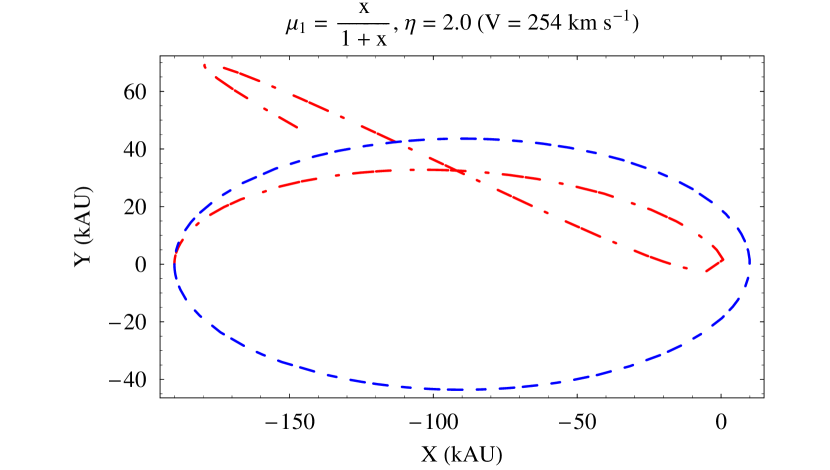
Figure 15: Numerically integrated orbits of an Oort comet with $a=100$ kAU, $e=0.9$, $P_{\rm b}=31.6$ Myr. Dashed blue line: Newton. Dash-dotted red line: MOND with $\mu_{1}$, $\eta=2.0$ ($V=254$ km s^-1). The initial conditions are $x_{0}=-a(1+e),y_{0}=z_{0}=0,\dot{x}_{0}=0,\dot{y}_{0}=-na\sqrt{\frac{1-e}{1+e}},\dot{z}_{0}=0$. The time span of the integration is $-P_{\rm b}\leq t\leq 0$.

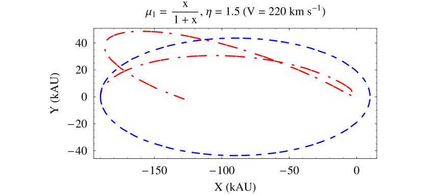
Figure 16: Numerically integrated orbits of an Oort comet with $a=100$ kAU, $e=0.9$, $P_{\rm b}=31.6$ Myr. Dashed blue line: Newton. Dash-dotted red line: MOND with $\mu_{1}$, $\eta=1.5$ ($V=220$ km s^-1). The initial conditions are $x_{0}=-a(1+e),y_{0}=z_{0}=0,\dot{x}_{0}=0,\dot{y}_{0}=-na\sqrt{\frac{1-e}{1+e}},\dot{z}_{0}=0$. The time span of the integration is $-P_{\rm b}\leq t\leq 0$.

3.2 Nearly polar orbits

Let us, now consider the case of orbits showing high inclinations $I$ to the ecliptic. For practical reasons, here we will only show some cases. In Figure 17-Figure 19 we depict the sections in the coordinate planes of an orbit with $a=66.6$ kAU, $e=0.92$, $I=81$ deg for $\mu_{1}$ and $\eta=1.5$. The initial conditions chosen are arbitrary in the sense that, contrary to Section 3.1, neither the perihelion nor the aphelion have been used as starting points.

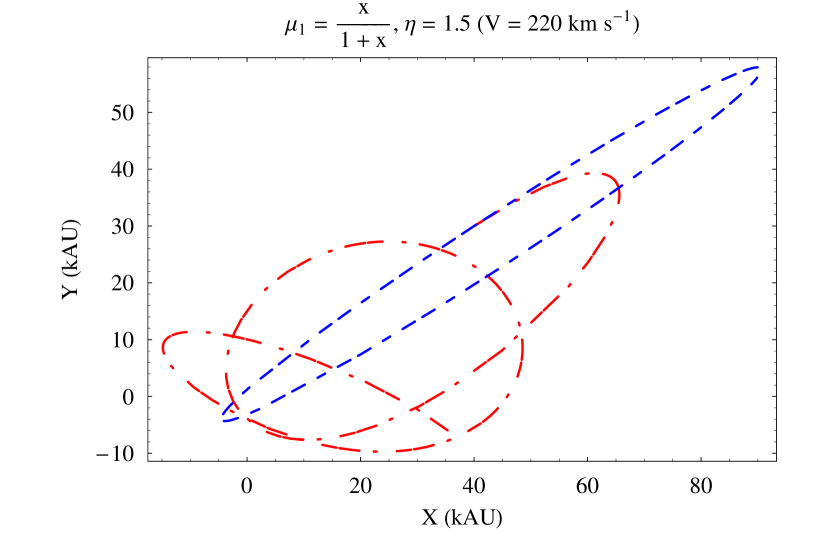
Figure 17: Section in the coordinate $\{\rm XY\}$ plane of the numerically integrated orbits of an Oort comet with $a=66.6$ kAU, $e=0.92$, $I=81$ deg. Dashed blue line: Newton. Dash-dotted red line: MOND with $\mu_{1}$, $\eta=1.5$ ($V=220$ km s^-1). The initial conditions are $x_{0}=40\ {\rm kAU},y_{0}=30\ {\rm kAU},z_{0}=5\ {\rm kAU},\dot{x}_{0}=-23\ {\rm kAU\ Myr^{-1}},\dot{y}_{0}=-15\ {\rm kAU\ Myr^{-1}},\dot{z}_{0}=-15\ {\rm kAU\ Myr^{-1}}$. The time span of the integration is $-P_{\rm b}\leq t\leq 0$.

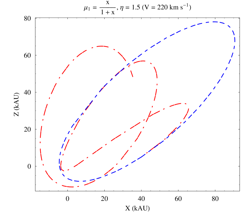
Figure 18: Section in the coordinate $\{\rm XZ\}$ plane of the numerically integrated orbits of an Oort comet with $a=66.6$ kAU, $e=0.92$, $I=81$ deg. Dashed blue line: Newton. Dash-dotted red line: MOND with $\mu_{1}$, $\eta=1.5$ ($V=220$ km s^-1). The initial conditions are $x_{0}=40\ {\rm kAU},y_{0}=30\ {\rm kAU},z_{0}=5\ {\rm kAU},\dot{x}_{0}=-23\ {\rm kAU\ Myr^{-1}},\dot{y}_{0}=-15\ {\rm kAU\ Myr^{-1}},\dot{z}_{0}=-15\ {\rm kAU\ Myr^{-1}}$. The time span of the integration is $-P_{\rm b}\leq t\leq 0$.

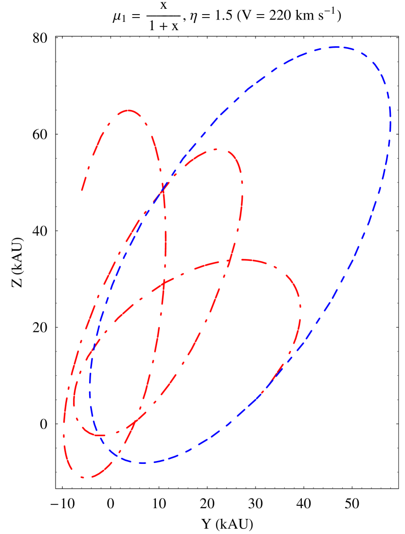
Figure 19: Section in the coordinate $\{\rm YZ\}$ plane of the numerically integrated orbits of an Oort comet with $a=66.6$ kAU, $e=0.92$, $I=81$ deg. Dashed blue line: Newton. Dash-dotted red line: MOND with $\mu_{1}$, $\eta=1.5$ ($V=220$ km s^-1). The initial conditions are $x_{0}=40\ {\rm kAU},y_{0}=30\ {\rm kAU},z_{0}=5\ {\rm kAU},\dot{x}_{0}=-23\ {\rm kAU\ Myr^{-1}},\dot{y}_{0}=-15\ {\rm kAU\ Myr^{-1}},\dot{z}_{0}=-15\ {\rm kAU\ Myr^{-1}}$. The time span of the integration is $-P_{\rm b}\leq t\leq 0$.

The case of $\mu_{3/2}$ and $\eta=1.5$ is illustrated in Figure 20- Figure 22.

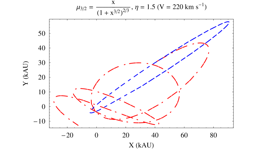
Figure 20: Section in the coordinate $\{\rm XY\}$ plane of the numerically integrated orbits of an Oort comet with $a=66.6$ kAU, $e=0.92$, $I=81$ deg. Dashed blue line: Newton. Dash-dotted red line: MOND with $\mu_{3/2}$, $\eta=1.5$ ($V=220$ km s^-1). The initial conditions are $x_{0}=40\ {\rm kAU},y_{0}=30\ {\rm kAU},z_{0}=5\ {\rm kAU},\dot{x}_{0}=-23\ {\rm kAU\ Myr^{-1}},\dot{y}_{0}=-15\ {\rm kAU\ Myr^{-1}},\dot{z}_{0}=-15\ {\rm kAU\ Myr^{-1}}$. The time span of the integration is $-P_{\rm b}\leq t\leq 0$.

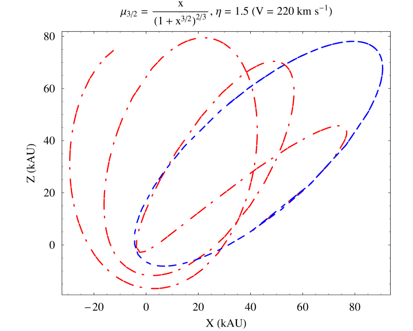
Figure 21: Section in the coordinate $\{\rm XZ\}$ plane of the numerically integrated orbits of an Oort comet with $a=66.6$ kAU, $e=0.92$, $I=81$ deg. Dashed blue line: Newton. Dash-dotted red line: MOND with $\mu_{3/2}$, $\eta=1.5$ ($V=220$ km s^-1). The initial conditions are $x_{0}=40\ {\rm kAU},y_{0}=30\ {\rm kAU},z_{0}=5\ {\rm kAU},\dot{x}_{0}=-23\ {\rm kAU\ Myr^{-1}},\dot{y}_{0}=-15\ {\rm kAU\ Myr^{-1}},\dot{z}_{0}=-15\ {\rm kAU\ Myr^{-1}}$. The time span of the integration is $-P_{\rm b}\leq t\leq 0$.

Figure 22: Section in the coordinate $\{\rm YZ\}$ plane of the numerically integrated orbits of an Oort comet with $a=66.6$ kAU, $e=0.92$, $I=81$ deg. Dashed blue line: Newton. Dash-dotted red line: MOND with $\mu_{3/2}$, $\eta=1.5$ ($V=220$ km s^-1). The initial conditions are $x_{0}=40\ {\rm kAU},y_{0}=30\ {\rm kAU},z_{0}=5\ {\rm kAU},\dot{x}_{0}=-23\ {\rm kAU\ Myr^{-1}},\dot{y}_{0}=-15\ {\rm kAU\ Myr^{-1}},\dot{z}_{0}=-15\ {\rm kAU\ Myr^{-1}}$. The time span of the integration is $-P_{\rm b}\leq t\leq 0$.

4 Consequences on the Oort cloud

The features of the MOND trajectories shown in the previous pictures suggest that EFE may have consequences on the interaction of the Oort-like objects with passing stars [20] by changing their perturbing effects and, thus, also altering the number of long-period comets launched into the inner regions of the solar system and the number of comets left in the cloud throughout its history. Indeed, in the standard picture, the comets moving along very (Newtonian) elongated orbits may come relatively close to a star of mass $M_{\star}$ suffering a change in velocity $\Delta v$ which approximately is [20]

$$\Delta v=\frac{2GM_{\star}}{v_{\star}d},$$ (27)

where $v_{\star}$ is the star’s velocity with respect to the Sun and $d$ is the distance of closest approach with the Oort object. Moreover, also the perturbing effects of the Galactic tides would be altered. In particular, for those particular initial configurations yielding highly shrunken paths with respect to the Newtonian case the perturbing effects of the passing stars and of the Galactic tides may get reduced. Anyway, it is very difficult to realistically predict the modifications that the Oort cloud would undergo under the action of MOND with EFE. Extensive numerical simulations like, e.g., the one in Ref. [36] performed in a different context, would be required; they are beyond the scope of the present paper.

5 Summary and conclusions

We investigated the orbital motions of test particles according to MOND with EFE in the Oort cloud ($r\approx 50-150$ kAU). As MONDian interpolating function $\mu(x)$, we extensively used the forms $\mu_{1}=1/(1+x),\mu_{2}=x/\sqrt{1+x^{2}},\mu_{3/2}=x/(1+x^{3/2})^{2/3}$. We numerically integrated both the MOND and the Newtonian equations of motion in Cartesian coordinates sharing the same initial conditions backward in time over one (Keplerian) orbital period. We considered both ecliptic and nearly polar trajectories, all corresponding to high (Newtonian) eccentricities ($e=0.5-0.9$). In order to evaluate the characteristic MONDian EFE parameters $\mu_{g}$ and $L_{g}$ entering the problem, we used two different values ($V=220$ km s^-1 and $V=254$ km s^-1) of the circular speed of the solar system’s motion through the Galaxy yielding the Milky Way’s gravitational field at the Sun’s location.

Our results show that the MOND orbits are quite different with respect to the Newtonian ones; in general, they are open trajectories which do not exhibit any regular patterns. Moreover, they are highly sensitive to the initial conditions in the sense that different sets of state vectors yielding the same Keplerian ellipses generate quite different MONDian paths. For certain initial configurations in the ecliptic, corresponding to Newtonian perihelion passages of highly eccentric orbits, the MOND trajectories reduce to intricate clews spanning very small spatial regions with respect to the Newtonian case. For other initial configurations, both in the ecliptic and outside it, the MOND trajectories are completely different: among other things, their spatial extensions are larger than in the ecliptic perihelion cases. As a consequence, the structure and the dynamical history of the Oort cloud, in the deep MONDian regime, would be altered with respect to the standard Newtonian picture in a way which is difficult to realistically predict.

As further extensions of the present work, which are outside its scope, we suggest that extensive numerical simulations of the dynamics of the Oort cloud in MOND with EFE would be helpful. Moreover, an analysis based on standard techniques of classical dynamics able to display regularities in orbits, like, e.g., surface of section, may be fruitfully implemented. Finally, let us note that a further issue which may be the subject of future investigations consists of the following. The numerically integrated MONDian trajectories with EFE may come close the Sun enough to fall in a Newtonian or quasi-Newtonian regime. If so, their further evolution should be obtained with a new integration of the Newtonian equations of motion starting from such new initial conditions. Consequently, the pattern of the Oort cloud may further change.

References

- [1] Bosma A. 21-cm line studies of spiral galaxies. I - Observations of the galaxies NGC 5033, 3198, 5055, 2841, and 7331. II - The distribution and kinematics of neutral hydrogen in spiral galaxies of various morphological types. The Astronomical Journal 1981; 86: 1791.
- [2] Rubin V.C., Ford W.K., Thonnard N., Burstein D. Rotational properties of 23 SB galaxies. The Astrophysical Journal 1982; 261: 439.
- [3] Rubin V.C. The Rotation of Spiral Galaxies. Science 1983; 220: 1339.
- [4] Milgrom M. A Modification of the Newtonian Dynamics as a Possible Alternative to the Hidden Mass Hypothesis. The Astrophysical Journal 1983a; 270: 365.
- [5] Milgrom M. A Modification of the Newtonian Dynamics - Implications for Galaxies. The Astrophysical Journal 1983b; 270: 371.
- [6] Milgrom M. A Modification of the Newtonian Dynamics - Implications for Galaxy Systems. The Astrophysical Journal 1983c; 270: 384.
- [7] Begeman K.G., Broeils A.H., Sanders R.H. Extended rotation curves of spiral galaxies - Dark haloes and modified dynamics. Monthly Notices of the Royal Astronomical Society 1991; 249: 523.
- [8] Famaey B., Binney J. Modified Newtonian dynamics in the Milky Way. Monthly Notices of the Royal Astronomical Society 2005; 363: 603.
- [9] Bekenstein J.D., Milgrom M. Does the Missing Mass Problem Signal the Breakdown of Newtonian Gravity?. The Astrophysical Journal 1984; 286: 7.
- [10] Zhao H., Famaey B. Refining the MOND Interpolating Function and TeVeS Lagrangian. The Astrophysical Journal 2006; 638: L9.
- [11] Famaey B., Gentile G., Bruneton J.-P., Zhao H. Insight into the baryon-gravity relation in galaxies. Physical Review D 2007; 75: 063002.
- [12] Sanders R.H., Noordermeer E. Confrontation of MOdified Newtonian Dynamics with the rotation curves of early-type disc galaxies. Monthly Notices of the Royal Astronomical Society 2007; 379: 702.
- [13] Brada R., Milgrom M. Exact solutions and approximations of MOND fields of disc galaxies. Monthly Notices of the Royal Astronomical Society 1995; 276: 453.
- [14] Bekenstein J.D. Relativistic gravitation theory for the modified Newtonian dynamics paradigm. Physical Review D 2004; 70: 083509.
- [15] Bruneton J.-P., Esposito-Farèse G. Field-theoretical formulations of MOND-like gravity. Physical Review D 2007; 76: 124012.
- [16] Zhao H. Coincidences of Dark Energy with Dark Matter: Clues for a Simple Alternative?. The Astrophysical Journal 2007; 671: L1.
- [17] Sanders R.H., McGaugh S.S. Modified Newtonian Dynamics as an Alternative to Dark Matter. Annual Review of Astronomy and Astrophysics 2002; 40: 263.
- [18] Bekenstein J.D. The modified Newtonian dynamics - MOND and its implications for new physics. Contemporary Physics 2006; 47: 387.
- [19] Milgrom M. The MOND paradigm. Talk presented at the xIx Rencontres de Blois Matter and energy in the Universe: from nucleosynthesis to cosmology, May 2007. Available from: http://arxiv.org/abs/0801.3133v2.
- [20] Oort J.H. The structure of the cloud of comets surrounding the solar system and a hypothesis concerning its origin. Bullettin of the Astronomical Institues of The Netherlands 1950; 11: 91.
- [21] Milgrom M. Solutions for the modified Newtonian dynamics field equation. The Astrophysical Journal 1986; 302: 617.
- [22] Talmadge C., Berthias J.-P., Hellings R.W., Standish E.M. Model-independent constraints on possible modifications of Newtonian gravity. Phyisical Review Letters 1988; 61: 1159.
- [23] Sereno M., Jetzer Ph. Dark matter versus modifications of the gravitational inverse-square law: results from planetary motion in the solar system. Monthly Notices of the Royal Astronomical Society 2006; 371: 626.
- [24] Bekenstein J.D., Magueijo J. Modified Newtonian dynamics habitats within the solar system. Physical Review D 2006; 73: 103513.
- [25] Sanders R.H. Solar system constraints on multifield theories of modified dynamics. Monthly Notices of the Royal Astronomical Society 2006; 370: 1519.
- [26] Ignatiev A.Yu. Is Violation of Newton’s Second Law Possible?. Physical Review Letters 2007; 98: 101101.
- [27] Iorio L. Constraining MOND with solar system dynamics. Journal of Gravitational Physics 2008; 2: 26.
- [28] Ignatiev A.Yu. Newton’s second law versus modified-inertia MOND: A test using the high-latitude effect. Physical Review D 2008; 77: 102001.
- [29] Iorio L. On the MOND external field effect in the solar system. Astrophysics and Space Science 2009; 323: 215.
- [30] Pitjeva E.V. Astronomy Letters 2005; 31: 340.
- [31] Folkner W.M. Relativistic aspects of the JPL planetary ephemeris. In: Klioner S.A., Seidelman P.K., Soffel M.H., Eds. Relativity in Fundamental Astronomy: Dynamics, Reference Frames, and Data Analysis, Proceedings of the International Astronomical Union, IAU Symposium, Volume 261. Cambridge University Press: Cambridge 2010; pp. 155-158.
- [32] Milgrom M. MOND effects in the inner solar system. Monthly Notices of the Royal Astronomical Society 2009; 399: 474.
- [33] Iorio L. The perihelion precession of Saturn, planet X/Nemesis and MOND. The Open Astronomy Journal 2010; 3: 1.
- [34] Commission 33 (Structure and Dynamics of the Galactic System/Structure et Dynamique du Syst‘eme Galctique) at the XIX General Assembly, Dehli, India, 1985. http://www.iau.org/static/resolutions/IAU1985French.pdf
- [35] Reid M.J., Menten K.M., Zheng X.W., Brunthaler A., Moscadelli L., Xu Y., Zhang B., Sato M., Honma M., Hirota T., Hachisuka K., Choi Y.K., Moellenbrock G.A., Bartkiewicz A. Trigonometric Parallaxes of Massive Star Forming Regions: VI. Galactic Structure, Fundamental Parameters and Non-Circular Motions. The Astrophysical Journal 2009; 700: 137.
- [36] Masi M., Secco L., Gonzalez G. Effects of the Planar Galactic Tides and Stellar Mass on Comet Cloud Dynamics. The Open Astronomy Journal 2009; 2: 74.