Cognitive computation with autonomously active neural networks: an emerging field

Abstract

The human brain is autonomously active. To understand the functional role of this self-sustained neural activity, and its interplay with the sensory data input stream, is an important question in cognitive system research and we review here the present state of theoretical modelling.

This review will start with a brief overview of the experimental efforts, together with a discussion of transient vs. self-sustained neural activity in the framework of reservoir computing. The main emphasis will be then on two paradigmal neural network architectures showing continuously ongoing transient-state dynamics: saddle point networks and networks of attractor relics.

Self-active neural networks are confronted with two seemingly contrasting demands: a stable internal dynamical state and sensitivity to incoming stimuli. We show, that this dilemma can be solved by networks of attractor relics based on competitive neural dynamics, where the attractor relics compete on one side with each other for transient dominance, and on the other side with the dynamical influence of the input signals.

Unsupervised and local Hebbian-style online learning then allows the system to build up correlations between the internal dynamical transient states and the sensory input stream. An emergent cognitive capability results from this set-up. The system performs online, and on its own, a non-linear independent component analysis of the sensory data stream, all the time being continuously and autonomously active. This process maps the independent components of the sensory input onto the attractor relics, which acquire in this way a semantic meaning.

1 INTRODUCTION

The brain has a highly developed and complex self-generated dynamical neural activity, and this fact raises a series of interesting issues. Does this self-sustained neural dynamics, its eigendynamics, have a central functional role, organizing overall cognitive computational activities? Or does this ongoing autonomous activity just serve as a kind of background with secondary computational task, like non-linear signal amplification or time encoding of neural codes?

The answer to this question is important not only to system neurobiology, but also for research in the field of cognitive computation in general. We will review here approaches based on the notion that the autonomous neural dynamics has a central regulating role for cognitive information processing. We will then argue, that this line of research constitutes an emerging field in both computational neuroscience and cognitive system research.

Some preliminaries, before we start. This is a mostly non-technical review with emphasis on content, an exhaustive and complete discussion of the published work on the subject is not the objective here. Centrally important equations will be given and explained, but for the numerical values of the parameters involved, and for the details of the simulation set-ups, we will refer to the literature. The discussion will be given generally from the perspective of cognitive system theory, viz bearing in mind the overall requirements of prospective complete cognitive systems, akin to ones of real-world living animals grosBook2008 ; grosEmo09 .

1.1 Autonomous brain dynamics

On the experimental side, the study of self-induced or autonomous neural activity in the brain has seen several developments in recent years, especially by fMRI studies fox2007 , and we will start by discussing some key issues arising in this respect.

The vast majority of experiments in cognitive neuroscience study the evoked neural response to certain artificial or natural sensory stimuli, often involving a given task which has been trained previously. It has been realized early on, that the neural response shows strong trial-to-trial variation, which is often as large as the response itself. This variability in the response to identical stimuli is a consequence of the ongoing internal neural activities (for a discussion see arieli1996 ). Experimentally one has typically no control over the details of the internal neural state and it is custom to consider it as a source of noise, averaging it out by performing identical experiments many times over. It is on the other side well known that the majority of energy consumption of the brain is spent on internal processes raichle2006 , indicating that the ongoing and self-sustained brain dynamics has an important functional role. Two possibilities are currently discussed:

(A) – The internal neural activity could be in essence a random process with secondary functional roles, such as non-linear signal amplification or reservoir computing for the spatiotemporal encoding of neural signals (for a theory review see vogels2005 ).

(B) – The internal neural activity could represent the core of the cognitive information processing, being modulated by sensory stimuli, but not directly and forcefully driven by the input signals. Indications for this scenario arise, e.g., from studies of the visual information processing fiser2004 and of the attention system fox2006 .

The overall brain dynamics is still poorly understood and both possibilities (A) and (B) are likely to be relevant functionally in different areas. In this review we will focus on the ramifications resulting from the second hypothesis. There are indications, in this regard, that distinct classes of internal states generated autonomously correspond to dynamical switching cortical states, and that the time series of the spontaneous neural activity patterns is not random but determined by the degree of mutual relations kenet2003 . Additionally, these spontaneous cortical state may be semantic in nature, having a close relation to states evoked by sensory stimuli ringach2003 and to neural activity patterns induced via thalamic stimulation maclean2005 . A second characteristics recurrently found in experimental studies is the organization of the spontaneously active states into spatially anticorrelated networks fox2005 , being transiently stable in time, in terms of firing rates, with rapid switching between subsequent states abeles1995 .

These results indicate that certain aspects of the time evolution of the self-sustained neural activity in the brain have the form of transient state dynamics, which we will discuss in detail in Sect. 2, together with a high associative relation between subsequent states of mind. This form of spontaneous cognitive process has been termed ‘associative thought process’ gros2005 .

It is currently under debate which aspects of the intrinsic brain dynamics is related to consciousness. The global organization of neural activity in anticorrelated and transiently stable states has been suggested, on one side, to be of relevance also for the neural foundations of consciousness edelman2000 ; edelman2003 , viz the ‘observing self’ baars2003a . The persistent default-mode network (for a critical perspective see morcom2007 ), viz the network of brain areas active in the absence of explicit stimuli processing and task performance, has been found, on the other side, to be active also under anesthetization vincent07 and light sedation greicius2008 . It is interesting to note, in this context, that certain aspects of the default resting mode can be influenced by meditational practices pagnoni2008 .

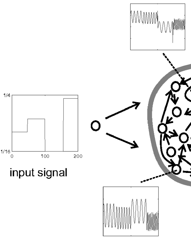
Figure 1: Operating principle of reservoir dynamics. The reservoir is activated by the input signal, mapping it in time and space to a higher-dimensional space. The reservoir activity provides then the basis for linear and supervised training of the output units, typically for time prediction tasks (figure courtesy H. Jaeger).

1.2 Reservoir computing

The term ‘neural transients’ characterizes evoked periods of neural activities, remaining transiently stable after the disappearance of the primary stimulating signal. In the prolonged absence of stimuli, neural architectures based on neural transients relax back to the quiescent default state. Network setups based on neural transients therefore occupy a role functionally in between pure stimulus-response architectures and systems exhibiting continuously ongoing autonomous neural activity. An important class of neural architectures based on neural transients are neural reservoirs, which we discuss now briefly.

A recurrent neural net is termed a reservoir, if it is not involved in the primary cognitive information processing, having a supporting role. A typical architecture is illustrated in Fig. 1. The reservoir is a randomly connected network of artificial neurons which generally has only a transiently stable activity in the absence of inputs, viz the reservoir has a short-term memory.

In the standard mode of operation an input signal stimulates the network, giving raise to complex spatiotemporal reservoir activities. Normally, there is no internal learning inside the reservoir, the intra-reservoir synaptic strengths are considered fixed. Time prediction is the standard application range for reservoir computing. For this purpose the reservoir is connected to an output layer and the activities of the output neurons are compared to a teaching signal. With supervised learning, either online or off-line, the links leading from the reservoir to the output then acquire a suitable synaptic plasticity.

There are two basic formulations of reservoir computing. The ‘echo-state’ approach using discrete-time rate-encoding neurons jaeger2001 ; jaeger2004 , and the ‘liquid state machine’ using continuous-time spiking neurons maass2002 ; maass2004 . In both cases the dimensionality of the input signal, consisting normally of just a single line, is small relative to the size of the reservoir, which may contain up to a few hundred neurons. Many nonlinear signal transformations are therefore performed by the reservoir in parallel and the subsequent perceptron-like output neurons may solve complex tasks via efficient linear learning rules.

Neural reservoirs are possible candidates for local cortical networks like microcolumns. The bare-bones reservoir network is not self-active, but feedback links from the output to the reservoir may stabilize ongoing dynamical activity maass2007 . In any case, reservoir nets are examples of network architectures of type (A), as defined in the previous section. The task of the reservoir, non-linear signal transformation, is performed automatically and has no semantic content. All information is stored in the efferent synaptic links.

There is an interesting similarity, on a functional level, of reservoir computing with the notion of a ‘global workspace’ baars2003b ; dehaene2003 . The global workspace has been proposed as a global distributed computational cortical reservoir, interacting with a multitude of peripheral local networks involving tasks like sensory preprocessing or motor output. The global workspace has also been postulated to have a central mediating role for conscious processes baars2003b ; dehaene2003 , representing the dominating hub nodes of a large-scale, small-world cortical network shanahan2007 .

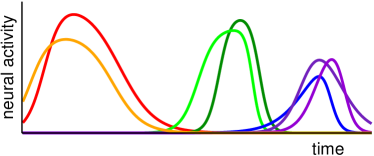
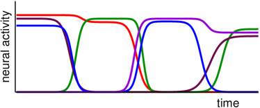
Figure 2: Two examples of transient state dynamics. Left: Bump-like phases of activities typically result from trajectories passing close to saddle points. Right: Transient states with pronounced plateaus are typical for multi-winners-take-all set-ups in the context of networks with attractor relics.

2 TRANSIENT STATE DYNAMICS

A central question in neuroscience regards the neural code, that is the way information is transmitted and encoded (see shadlen1998 ; eggermont1998 for reviews). Keeping in mind that there is probably no pure information transmission in the brain, as this would be a waste of resources, that information is also processed when transmitted, one may then distinguish two issues regarding the encoding problem.

On one hand there is the question on how sensory signals are reflected, on relative short timescales, in subsequent neural activities. Available neural degrees of freedom for this type of short-time encoding are the average firing rates (rate encoding), transient bursts of spikes and the temporal sequence of spikes (temporal encoding). In addition, the response of either individual neurons may be important, or the response of local ensembles eggermont1998 ; averbeck2004 .

The subsequent sensory signal processing, on timescales typically exceeding 25-100ms, may, on the other hand, involve neural dynamics in terms of transiently stable activity patterns, as discussed earlier in Sect. 1.1. In Fig. 2 two types of model transient state activities are illustrated. Alternating subsets of neurons are either active, to various degrees, or essentially silent, resulting in well characterized transient states having a certain degree of discreteness. This discreteness should be reflected, on a higher level, on the properties of the corresponding cognitive processes. Of interest in this context is therefore the ongoing discussion, whether visual perception is continuous or discrete in the time domain vanrullen2003 ; kline2004 , on timescales of the order of about 100ms, with the discrete component of perception possibly related to object recognition vanrullen2006 . Transient state dynamics in the brain may therefore be related to semantic recognition, a connection also found in models for transient state dynamics based on competitive neural dynamics. In the following we will examine the occurrence and the semantic content of autonomous transient state dynamics in several proposed cognitive architectures.

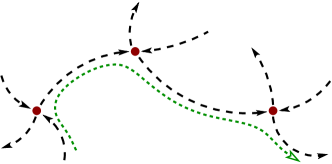
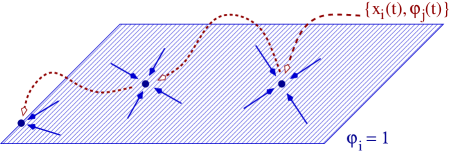
Figure 3: Two scenarios giving rise to transient state dynamics. Left: A network of saddle points (filled circles) connected via heteroclines (long dashed lines) with a sample trajectory (short-dashed line). The dynamics slows down close to a saddle point. Right: An attractor network (shaded plane) is embedded in a higher dimensional space via additional reservoir variables $\{\varphi_{j}(t)\}$, leading to a destruction of the original fixpoints (filled circles), which are turned into attractor relics. The dynamics $\{x_{i}(t),\varphi_{j}(t)\}$ (short-dashed line) slows down in the vicinity of an attractor relic.

2.1 Saddle point networks and winnerless competition

The concept of saddle point networks is based on the premises, (a) that the internal ongoing autonomous dynamics organizes the cognitive computation and (b) that the cognitive behavior is reproducible and deterministic in identical environments rabinovich2008 . As we will discuss in the next section, the first assumption is shared with attractor relic networks, while the second is not.

Technically, one considers a dynamical system, viz a set of $N$ first-order differential equations and the set of the respective saddle points, compare Fig. 3. The precondition is now that every saddle point has only a single unstable direction and $(N-1)$ stable directions. Any trajectory approaching the saddle point will then leave it with high probability close to the unique unstable separatrix and the system therefore has a unique limiting cycle attractor. This limiting cycle does not need to be a global attractor, but normally has a large basin of attraction. During one passage most, if not all, saddle points are visited one after the other, giving raise to a transient state dynamics illustrated in Fig. 2, with the trajectory slowing down close to a saddle point.

Another condition for this concept to function is the formation of a heteroclinic cycle, which is of a set in phase space invariant under time evolution krupa1997 . Implying, as illustrated in Fig. 3, that the unstable separatrix of a given saddle point needs to end up as a stable separatrix of another saddle point. Such a behavior occurs usually only when the underlying differential equations are invariant under certain symmetry operations, like the exchange of variables krupa1997 . For any practical application, these symmetries need to be broken and the limiting cycle will vanish together with the heteroclinic sequence. It can however be restored in form of a heteroclinic channel, if the strength of the symmetry-breaking is not too strong, by adding a stochastic component to the dynamics. With noise, a trajectory loitering around a saddle point can explore a finite region of phase space close to the saddle point until it finds the unstable direction. Once the trajectory has found stochastically the unstable direction, it will leave the saddle point quickly along this direction in phase space and a heteroclinic channel is restored functionally. Cognitive computation on the backbone of saddle point networks is therefore essentially based on an appropriate noise level.

Cognitive computation with saddle point networks has been termed ‘winnerless competition’ in the context of time encoding of natural stimuli rabinovich2001 and applied to the decision making problem. In the later case interaction with the environment may generate a second unstable direction at the saddle points and decision taking corresponds to the choice of unstable separatrix taken by the trajectory rabinovich2008 .

2.2 Attractor relic networks and slow variables

A trivial form of self-sustained neural activity occurs in attractor networks amit89 . Starting with any given initial state the network state will move to the next attractor and stay there, with all neurons having a varying degree of constant firing rates, the very reason attractor nets have been widely discussed as prototypes for the neural memory hasselmo99 . As such, an attractor network is useless for a cognitive system, as it needs outside help, or stimuli from other parts of the system, to leave the current attractor.

There is a general strategy which transforms an attractor network into one exhibiting transient state dynamics, with the transient neural states corresponding to the fixpoints of the original attractor network. This procedure is applicable to a wide range of attractor networks and consists in expanding the phase space by introducing additional local variables akin to local activity reservoirs gros2005 .

To be concrete, let us denote with $\{x_{i}\}$ the set of dynamical variables of the attractor network, as illustrated in Fig. 3, and by $\{\varphi_{j}\}$ the additional reservoir variables. We assume that the reservoirs are depleted / filled when the neuron is active / inactive,

$$T_{\varphi}\,\dot{\varphi}_{j}(t)\ \to\ \left\{\begin{array}[]{rcl}<0&&{\rm active\ neuron}\ j\\ >0&&{\rm inactive\ neuron}\ j\end{array}\right.~{}.$$ (1)

Together with a suitable coupling of the reservoir variables $\{\varphi_{j}\}$ to the neural activities $\{x_{i}\}$ one can easily achieve that the fixpoints of the attractor networks become unstable, viz that they are destroyed, turning into attractor ruins or attractor relics.

This situation is illustrated in Fig. 3. In the expanded phase space $\{x_{i},\varphi_{j}\}$ there are no fixpoints left. It is not the case that the attractors would just acquire additional unstable directions, upon enlargement of the phase space, turning them into saddle points. Instead, the enlargement of the phase space destroys the original attractors completely. The trajectories will however still slow down considerably close to the attractor ruins, as illustrated in Fig. 2, if the reservoirs are slow variables, changing only relatively slowly with respect to the typical time constants of the original attractor network. In this case the time constant $T_{\varphi}$ entering the time evolution of the reservoir, Eq. (1), is large. In the limit $T_{\varphi}\to\infty$ the reservoir becomes static and the dynamics is reduced to the one of the original attractor network.

The dynamics exhibited by attractor relic networks is related to the notion of chaotic itinerancy tsuda2002 , which is characterized by trajectories wandering around chaotically in phase space, having intermittent transient periods of stability close to attractor ruins. Here we consider the case of attractor relics arising from destroyed point attractors. In the general case one may also consider, e.g., limit cycles or strange attractors.

The coupling to slow variables outlined here is a standard procedure for controlling dynamical systems grosBook2008 , and has been employed in various fashions for the generation and stabilization of transient state dynamics. One possibility is the use of dynamical thresholds for discrete-time rate-encoding neural nets horn1989 . In this case one considers as a slow variable the sliding-time averaged activity of a neuron and the threshold of a neuron is increased / decreased whenever the neuron is active / inactive for a prolonged period. Another approach is to add slow components to all synaptic weights for the generation of an externally provided temporal sequence of neural patterns sompolinsky1989 . In the following we will outline in some detail an approach for the generation of transient state dynamics which takes an unbiased clique encoding neural net as its starting point gros2007 , with the clique encoding network being a dense and homogeneous associative network (dHan).

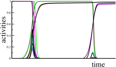
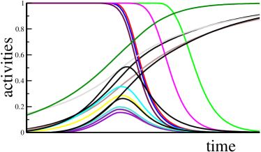
Figure 4: Multi-winners-take-all transient state dynamics and neural competition. The right graph is a blow-up of the first transition in the left graph. During the transition many neurons compete with each other for becoming a member of the next winning coalition. The duration of the transient-state plateaus is given by the relaxation time $T_{\varphi}$ of the slow variables, see Eq. (1).

3 COMPETITIVE NEURAL DYNAMICS

Transient state dynamics is intrinsically competitive in nature. When the current transient attractor becomes unstable, the subsequent transient state is selected via a competitive process. Transient-state dynamics is a form of ‘multi-winners-take-all’ process, with the winning coalition of dynamical variables suppressing all other competing activities maass2000 ; oreilly1998 . Competitive processes resulting in quasi-stationary states with intermittent burst of changes are widespread, occurring in many spheres of the natural or the social sciences. In the context of Darwinian evolution, to give an example, this type of dynamics has been termed ‘punctuated equilibrium’ grosBook2008 . In the context of research on the neural correlates of consciousness, these transiently stable states in form of winning coalitions of competing neural ensembles have been proposed as essential building blocks for human states of the mind crick2003 ; koch2004 .

The competitive nature of transient state dynamics is illustrated in Fig. 4, where a representative result of a simulation for a dHan net is presented. During the transition from one winning coalition to the subsequent, many neurons try to become members of the next winning coalition, which in the end is determined by the network geometry, the synaptic strengths and the current reservoir levels of the participating neurons.

The transition periods from one transient state to the next are periods of increased dynamical sensibility. When coupling the network to sensory inputs, the input signal may tilt the balance in this competition for the next winning coalition, modulating in this way the ongoing internal dynamical activity. Transient state dynamics therefore opens a natural pathway for implementing neural architectures for which, as discussed in the introduction, the eigendynamics is modulated, but not driven, by the sensory data input stream. A concrete example of how to implement this procedure will be discussed in Sect. 4.

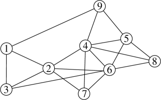
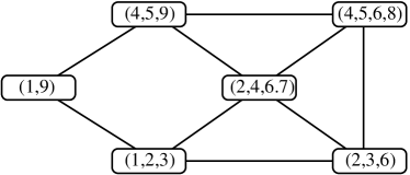
Figure 5: Clique encoding. On the left a 9-site network. On the right the 5 cliques contained in the left-side network are given. The cliques are connected via edges whenever they share one or more sites and can therefore be considered as the constituent vertices of a meta network of cliques.

3.1 Clique encoding

Only a small fraction of all neurons are active at any time in the brain in general, and in areas important for the memory consolidation in particular quiroga2008 . For various reasons, like the optimization of energy consumption and the maximization of computational capabilities olshausen2004 , sparse coding is an ubiquitous and powerful coding strategy maass2000 . Sparse coding may be realized in two ways, either by small non-overlapping neural ensembles, as in the single-winner-take-all architecture, or by overlapping neural ensembles. The latter pathway draws support from both theory considerations quiroga2008 , and from experimental findings.

Experimentally, several studies of the Hippocampus indicate that overlapping neural ensembles constitute important building blocks for the real-time encoding of episodic experiences and representations lin2005 ; lin2006 . These overlapping representations are not random superpositions but associatively connected. A hippocampal neuron could response, e.g., to various pictures of female faces, but these pictures would tend to be semantically connected, e.g. they could be the pictures of actresses from the same TV series quiroga2005 . It is therefore likely that the memory encoding overlapping representations form an associative network, a conjecture that is also consistent with studies of free associations nelson2004 ; palla2005 .

There are various ways to implement overlapping neural encoding with neural nets. Here we discuss the case of clique encoding. The term clique stems from graph theory and denotes, just as a clique of friends, a subgraph where (a) every member of the clique is connected with all other members of the clique and where (b) all other vertices of the graph are not connected to each member of the clique. In Fig. 5 a small graph is given together with all of its cliques.

Also shown in Fig. 5 are the associative interconnections between the cliques. One may view the resulting graph, with the cliques as vertices and with the inter-clique associative connections as edges, as a higher-level representation of an implicit hierarchical object definition riesenhuber1999 . The clique (4,5,9) in the original graph in Fig. 5 corresponds to a primary object and the meta-clique [(4,5,9)-(2,4,6,7)-(4,5,6,8)] in the graph of the cliques would in this interpretation encode a meta object, composed of the primary objects (4,5,9), (2,4,6,7) and (4,5,6,8). This intrinsic possibility of hierarchical object definitions when using clique encoding has however not yet be explored in simulations and may be of interest for future studies.

Cliques can be highly overlapping and there can be a very large number of cliques in any given graph kaczor2008 ; grosKaczor2008 . We will construct now a neural net where the cliques of the network are the attractors. It is a homogeneously random and dense associative network (dHan), where the associative relations between cliques are given by the number of common vertices. Starting from this attractor network we will introduce slow variables, as discussed in Sect. 2.2, in terms of local reservoirs. The network will then show spontaneously generated transient state dynamics, with the neural cliques as the attractor ruins. In a second step we will couple the dHan net to sensory stimuli and study the interplay between the internal autonomous dynamical activity and the data input stream. We will find that the cliques acquire semantic content in this way, being mapped autonomously to the statistically independent patterns of the data input stream.

3.2 Attractor network

The starting point of our considerations is the underlying attractor network, for which we employ a continuous time formulation, with rate encoding neurons, characterized by normalized activity levels $x_{i}\in[0,1]$. The growth rates $r_{i}$ govern the respective time developments,

$$\dot{x}_{i}\ =\ \left\{\begin{array}[]{rcl}(1-x_{i})\,r_{i}&&(r_{i}>0)\\ x_{i}\,r_{i}&&(r_{i}<0)\end{array}\right.~{}.$$ (2)

When $r_{i}>0$, the respective neural activity $x_{i}$ increases, approaching rapidly the upper bound; when $r_{i}<0$, it decays to zero. We split the rates into three contributions:

$$r_{i}\ =\ r_{i}^{(+)}\,+\,r_{i}^{(-)}\,+\,r_{i}^{(ext)}~{}.$$ (3)

An internal positive contribution $r_{i}^{(+)}\geq 0$, an internal negative contribution $r_{i}^{(-)}\leq 0$, and the influence of external stimuli, $r_{i}^{(ext)}$. We will discuss the influence of non-trivial external stimuli in Sect. 4, for the moment we consider $r_{i}^{(ext)}\equiv 0$. The division into an exciting and a depressing contribution in Eq. (3) reflects on one side the well known asymmetry between excitatory neurons and inhibitory interneurons in the brain arbib2002 and is on the other side essential for clique encoding. The $r_{i}^{(+)}$ are determined via

$$r_{i}^{(+)}\ =\ f_{w}(\varphi_{i})\sum_{j}w_{ij}\,x_{j}$$ (4)

by the influence of the excitatory synaptic weights, $w_{ij}\geq 0$. The function $f_{w}(\varphi)$ entering Eq. (4) couples the dynamics of the neurons locally to the slow variables $\varphi_{i}$. We will examine the reservoir function $f_{w}(\varphi)$ in the next Section. For the time being we set $f_{w}(\varphi)\equiv 1$, the primary neural dynamics is then decoupled from the reservoir dynamics and we will retain the starting attractor network. The $r_{i}^{(-)}\leq 0$ are given by

$$r_{i}^{(-)}\ =\ z\,\tanh\left(\sum_{j}z_{ij}\,x_{j}\,f_{z}(\varphi_{j})\right)~{},$$ (5)

where the $z_{ij}\leq 0$ are the inhibitory synaptic weights and where $z>0$ sets the scale for the inhibition. Eq. (5) leads to a normalization $-z<r_{i}^{(-)}\leq 0$. We postpone the discussion of the reservoir function $f_{z}(\varphi)$ and consider for the time being $f_{z}(\varphi)\equiv 1$.

Clique encoding corresponds to a multi-winners-take-all formulation. An inhibitory background is therefore necessary. The dHan architecture contains hence an inhibitory link $z_{ij}$ whenever there is no excitatory link $w_{ij}$,

$$z_{ij}\ =\ \left\{\begin{array}[]{rcl}-z&&(w_{ij}=0)\\ 0&&(w_{ij}>0)\end{array}\right.~{},$$ (6)

viz the excitatory links are shunting the inhibitory synapses. This inhibitory background is implicitly present for the 9-site network shown in Fig. 5. The edges of the network shown in Fig. 5. correspond to excitatory links $w_{ij}>0$. All pairs of sites not connected by an edge in Fig. 5 inhibit each other via $z_{ij}<0$.

The formulation of the attractor network with clique encoding is such complete gros2007 . All members of a given clique excite each other via intra-clique $w_{ij}>0$. Neurons which are not members of the current active clique are suppressed by at least one inhibitory link $z_{ij}<0$. This suppression $\sim(-z)$, compare Eq. (5), dominates the residual positive signal the out-of-clique neuron may receive, whenever $z$ is large enough.

An interesting feature of the dHan architecture is the absence of a bias in Eq. (2). There is no self excitation or suppression, $w_{ii}=z_{ii}=0$. The dynamics of an individual neuron is exclusively driven by the influence of the network, it has no preferred firing state. This feature would correspond for real-world neurons to the existence of a background of afferent activities with a level close to the firing threshold.

Next we note, that the separation of scales $z\gg w_{ij}$ implies that Hebbian-type modification of the inhibitory links $z_{ij}$ would be meaningless, small changes of a relatively large quantity will not lead to a substantial effect. Hebbian learning in the dHan architecture is therefore operational only for the excitatory links $w_{ij}$, in accordance to the general assumption that most learning taking place in the brain involves synapses interconnecting neurons and not interneurons arbib2002 . In Sect. 4 we will consider the synaptic plasticity of links afferent to the dHan layer. Unsupervised and local Hebbian-style learning can however be implemented easily for the intra-dHan excitatory links $w_{ij}$ for unsupervised and homeostatic calibration of the excitatory links gros2007 . It is however not essential for the occurrence and for the stabilization of transient state dynamics, our focus here.

3.3 Reservoir activity

We consider normalized slow variables $\varphi_{i}\in[0,1]$, with the time evolution

$$\dot{\varphi}_{i}(t)\,=\,r_{\varphi_{i}}^{av}+{1\over T_{\varphi}}\left\{\begin{array}[]{ccl}-\varphi_{i}&&{\rm active\ neuron}\ i\\ (1-\varphi_{i})&&{\rm inactive\ neuron}\ i\end{array}\right.~{},$$ (7)

where a neuron is active / inactive whenever its activity level $x_{i}$ is close to unity / zero. The $\varphi_{i}$ behave functionally as reservoirs, being depleted / refilled for active / inactive neurons. The term $r_{\varphi_{i}}^{av}$ on the RHS of Eq. (7) is not essential for the establishment of transient state dynamics, but opens an interesting alternative interpretation for the slow variables. $r_{\varphi_{i}}^{av}$ vanishes for inactive neurons and takes the value

$$r_{\varphi_{i}}^{av}\big{|}_{{\rm active}\ i}\ =\ {1\over T_{\varphi}^{av}}\sum_{{\rm active}\ j}\left(\varphi_{j}-\varphi_{i}\right)$$ (8)

for active neurons. The reservoir levels $\{\varphi_{i}\}$ of all active neurons are drawn together consequently. All members of the currently active winning coalition have then similar reservoir levels after a short time, on the order of $T_{\varphi}^{av}$. This is a behavior similar to what one would expect for groups of spiking neurons forming winning coalitions via synchronization of their spiking times. For each neuron of the winning coalitions one could define a degree of synchronization, given by the extent this neuron contributes to the overall synchronization. Initially, this degree of synchronization would have a different value for each participating neuron. On a certain timescale, denoted here by $T_{\varphi}^{av}$, the spiking times would then get drawn together, synchronized, and all members of the winning coalition of active neurons would then participate to a similar degree in the synchronized firing. The firing of the winning coalition would however not remain coherent forever. Internal noise and external influences would lead to a desynchronization on a somewhat longer time scale $T_{\varphi}\gg T_{\varphi}^{av}$. When desynchronized, the winning coalition would loose stability, giving way to a new winning coalition. In this interpretation the reservoirs allow for a “poor man’s” implementation of self organized dynamical synchronization of neural ensembles, a prerequisite for the temporal coding hypothesis of neural object definition vonDerMalsburg1999 ; singer1995 .

Finally we need to specify the reservoir coupling functions $f_{w}(\varphi)$ and $f_{z}(\varphi)$ entering Eqs.  (4) and (5). They have sigmoidal form with

$$f_{w}(\varphi),\ f_{z}(\varphi)\ \to\ \left\{\begin{array}[]{rcl}\sim 1&&\varphi\to 1\\ \sim 0&&\varphi\to 0\end{array}\right.~{},$$ (9)

and a straightforward interpretation: It is harder to excite a neuron with depleted reservoir, compare Eq.  (4), and a neuron with a low reservoir level has less power to suppress other neurons, see Eq.  (5). Reservoir functions obeying the relation (9) therefore lead in a quite natural way to transient state dynamics. On a short time scale the system relaxes towards the next attractor ruin in the form of a neural clique. Their reservoirs then slowly decrease and when depleted they can neither continue to mutually excite each other, nor can they suppress the activity of out-of-clique neurons anymore. At this point, the winning coalition becomes unstable and a new winning coalition is selected via a competitive process, as illustrated in Fig. 4.

Any finite $T_{\varphi}<\infty$ leads to the destruction of the fixpoints of the original attractor network, which is thus turned into an attractor relic network. The sequence of winning coalitions, given by the cliques of the network, is however not random. Subsequent active cliques are associatively connected. The clique (1,9) of the 9-site network shown in Fig. 5, to give an example, could be followed by either (4,5,9) or by (1,2,3), since they share common sites. The competition between these two cliques will be decided by the strengths of the excitatory links and by the history of previous winning coalitions. If one of the two cliques had been activated recently, the constituent sites will still have a depressed reservoir and resist a renewed reactivation.

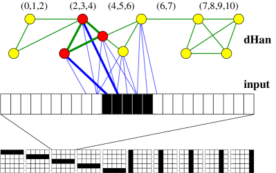
Figure 6: A dHan layer (top) with neural activities $\{x_{i}\}$ and cliques (0,1,2), … receives sensory signals via the input layer (middle) in the form of certain input patterns (bottom).

The finite state dynamics of the dHan architecture is robust. For the isolated network, we will discuss the coupling to sensory input in the next section, the dynamics is relaxational and dissipative gros2007 . The system relaxes to the next attractor relic and the reservoirs are relaxing either to zero or to unity, depending on the respective neural activity levels. For a network with a finite number of sites, the long-time state will be a long limiting cycle of transient states.

The simulation results shown in Fig. 4 are for a set of parameters resulting in quite narrow transitions and long plateaus gros2007 . The formulation presented here allows for the modelling of the shape of the plateaus and of other characteristics of the transient state dynamics. A smaller $T_{\varphi}$ would result in shorter plateaus, a longer $T_{\varphi}^{av}$ in longer transition times. One can, in addition, adjust the shape of the reservoir functions and details of Eqs. (4) and (5) in order to tune the overall competition for the next winning coalition. The dHan architecture providing therefore a robust framework for the generation of transient state dynamics, offering at the same time ample flexibility and room for fine tuning, paving the way for a range of different applications.

4 INFLUENCE OF EXTERNAL STIMULI

The transient state dynamics generated by the dHan architecture is dynamically robust. The dHan dynamics has at the same time windows of increased sensibility to outside influences during the transition periods from one transient state to the subsequent, as shown in Fig. 4. These transition periods are phases of active inter-neural competition, reacting sensibly to the influence of afferent signals.

We couple the input signals via an appropriate input layer, as illustrated in Fig. 6, denoting by $y_{i}\in[0,1]$ the time dependent input signals, which we will take as black-and-white or grey-scaled patterns. We denote by $v_{ij}$ the afferent links to the dHan layer, with the external contribution to the dHan-layer growth rates, compare Eq. (3), given by

$$r_{i}^{(ext)} = \left\{\begin{array}[]{ccl}0&&{\rm neuron}\ i\ {\rm active\ and}\ \Delta r_{i}<0\\ \Delta r_{i}&&\end{array}\right.~{},$$ (12)

$$\Delta r_{i} = \sum_{j}v_{ij}\,y_{j}~{}.$$ (13)

The rationale behind this formulation is the following. The role of the input signal is not to destabilize the current winning coalition, the afferent signal is therefore shunted off in this case, Eq. (12). The input signal should influence the competition for the next winning coalition, modulating but not driving directly the dHan dynamics. This rational is realized by the above formulation. Inactive neurons will receive a bias $\Delta r_{i}$ from the input layer which increases / decreases its chance of joining the next winning coalition for $\Delta r_{i}>0$ / $\Delta r_{i}<0$.

4.1 Novelty signal

A cognitive system with a non-trivial and self-sustained internal neural activity has to decide how and when correlations with the sensory data input stream are generated via correlations encoded in the respective synaptic plasticities. This is clearly a central issue, since the input data stream constitutes the only source for semantic content for a cognitive system.

It makes clearly no sense if the afferent links to the dHan layer, viz the links leading from the input to the internal network supporting a self-sustained dynamical activity, would be modified continuously via Hebbian-type rules, since the two processes, the internal and the environmental dynamics, are per se unrelated. It makes however sense to build up correlation whenever the input has an influence on the internal activity, modulating the ongoing associative thought process. From the perspective of the cognitive system such a modulation of the internal dynamics by environmental stimuli corresponds to something novel and unexpected happening. Novelty detection is therefore vital for neural networks with a non-trival eigendynamics processing sensory data. The importance of novelty detection for human cognition has been acknowledged indeed since long berns1997 ; barcelo2002 , and a possible role of Dopamine, traditionally associated with reinforcement reward transmission wise2004 , for the signalling of novelty has been suggested recently redgrave2006 .

The influence of modulating and of not modulating sensory signals is illustrated in Fig. 7, where simulation results for a dHan layer containing seven neurons coupled to an intermittent input signal are presented. The signal is not able to deactivate a currently stable winning coalition, compare Eq. (13), but makes an impact when active during a transition period. The system has the possibility to figure out whenever the later has happened. When the input signal $r_{i}^{(ext)}$ is relevant then

$$\big{(}r_{i}>0\big{)}\qquad\mbox{and}\qquad\big{(}r_{i}^{(+)}+r_{i}^{(-)}<0\big{)}~{}.$$ (14)

In this case the internal contribution $r_{i}^{(+)}+r_{i}^{(-)}$ to the growth rate is negative and the input makes a qualitative difference. We may therefore define a global novelty signal $S=S(t)$ obeying

$$\dot{S}\ =\ \left\{\begin{array}[]{rcl}\phantom{-}1/T_{S}^{+}&&(r_{i}>0)\mbox{\ and\ }(r_{i}<r_{i}^{(ext)})\\ -1/T_{S}^{-}&&\mbox{otherwise}\end{array}\right.,$$

where we have used Eq. (3), $r_{i}^{(+)}+r_{i}^{(-)}=r_{i}-r_{i}^{(ext)}$, and where a $\sum_{i}$ is implicit on the RHS of the equation. The novelty signal needs to be activated quickly, with $T_{S}^{+}\gg T_{S}^{-}$. Learning then takes place whenever the novelty signal $S$ exceeds a certain threshold.

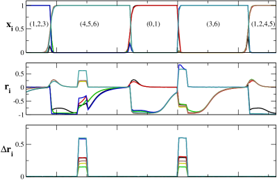
Figure 7: The activity levels $x_{i}$ of a dHan layer containing seven neurons, compare Fig. 6, the growth rates $r_{i}$ and the contributions from the input-layer $\Delta r_{i}$, see Eq. (13). The first input stimulus does not lead to a deviation of the transient state dynamics of the dHan layer. The second stimulus modulates the ongoing transient state dynamics, influencing the neural competition during the sensitive phase.

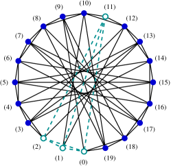
Figure 8: Top: The 20-site regular dHan net used for the bars problem. It contains 10 cliques with four vertices. The clique (0,1,2,11) is highlighted. Bottom: Some illustrative input patterns for the $5\times 5$ bars problem.

4.2 Afferent link plasticity: optimization principle

Having determined when learning takes place, we have now to formulate the rules governing how learning modifies the links afferent to the dHan layer. For this purpose we will use the Hebbian principle, that positive interneural correlations are enforced and negative correlations weakened. Our system is however continuously active, at no point are activities or synaptic strengths reset. The Hebbian principle therefore needs to be implemented as an optimization process bienenstock , and not as a maximization process, which would lead to a potentially hazardous runaway growth of synaptic strengths.

There are four quadrants in the $2\times 2$ Hebbian learning matrix, corresponding to active / inactive pre- and post-synaptic neurons, out of which we use the following three optimization rules:

(a) The sum over active afferent links leading to active dHan neurons is optimized to a large but finite value $r_{v}^{act}$,

$$\sum_{j}v_{ij}\,y_{j}\bigg{|}_{x_{i}\,{\rm active}}\ \to\ r_{v}^{act}~{}.$$

(b) The sum over inactive afferent links leading to active dHan neurons is optimized to a small value $s_{v}^{orth}$,

$$\sum_{j}v_{ij}\,(1-y_{j})\bigg{|}_{x_{i}\,{\rm active}}\ \to\ s_{v}^{orth}~{}.$$

(c) The sum over active afferent links leading to inactive dHan neurons is optimized to a small value $r_{v}^{ina}$,

$$\sum_{j}v_{ij}\,y_{j}\bigg{|}_{x_{i}\,{\rm inactive}}\ \to\ r_{v}^{ina}~{}.$$

The $r_{v}^{act}$, $r_{v}^{ina}$ and $s_{v}^{orth}$ are the target values for the respective optimization processes, where the superscripts stand for ‘active’, ‘inactive’ and ‘orthogonal’ gros2008_karl . These three optimization rules correspond to fan-in normalizations of the afferent synapses. Positive correlations are build up whenever $r_{v}^{act}$ dominates in magnitude, and orthogonalization of the receptive fields to other stimuli is supported by $s_{v}^{orth}$. A small but non-vanishing value for $r_{v}^{ina}$ helps to generate a certain, effective, fan-out normalization, avoiding the uncontrolled downscaling of temporarily not needed synapses.

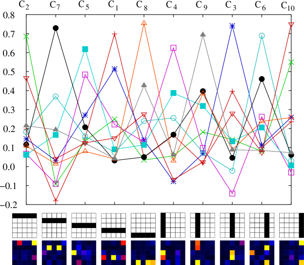
Figure 9: For the $5\times 5$ bars problem the response (see Eq. (15)), of the 10 cliques $C_{1},..,C_{10}$ in the dHan layer. The clique response is given with respect to the ten reference patterns, viz the 5 horizontal bars and the 5 vertical bars of the $5\times 5$ input field shown below the graph. In the top row the cliques with the maximal response to the respective reference patterns is given. In the bottom row, below each of the 10 black / white reference patterns, the receptive fields, Eq. (16), for the cliques $C_{\alpha}$ with the maximal susceptibility (given in the top row) are shown color-coded, with black/blue/red/yellow coding synaptic strengths of increasing intensities.

4.3 The bars problem

Knowledge about the environment lies at the basis of all cognition, before any meaningful action can be taken by a cognitive system. For simple organisms this knowledge is implicitly encoded in the genes, but in general a cognitive system needs to extract this information autonomously from the sensory data input stream, via unsupervised online learning. This task includes signal separation and features extraction, the identification of recurrently appearing patterns, i.e. of objects, in the background of fluctuation and of combinations of distinct and noisy patterns. For the case of linear signal superposition this problem is addressed by the independent component analysis hyvarinen2000 and blind source separation choi2005 , which seeks to find distinct representations of statistically independent input patterns. In order to examine how our system of an input layer coupled to a dHan layer, as illustrated in Fig. 6, analyzes the incoming environmental signals, we have selected the bars problem barsProblem ; butko2007 .

The bars problem constitutes a standard non-linear reference task for feature extraction via a non-linear independent component analysis for an $L\times L$ input layer. The basic patterns are the $L$ vertical and $L$ horizontal bars and the individual input patterns are made up of a non-linear superposition of the $2L$ basic bars, containing any of them with a certain probability $p$, typically $p\approx 0.1$, as illustrated in Fig. 8.

Our full system then consist of the dHan layer, which is continuously active, and an input layer coding the input patterns consisting of randomly superimposed black / white bars. For the dHan network we have taken a regular 20-site ring, containing a total of 10 cliques $C_{\alpha},\ \alpha=1..10$, each clique having $S(C_{\alpha})=4$ sites, as illustrated in Fig. 8. The self-sustained transient-state process is continuously active in the dHan layer, modulated by the contributions $\{\Delta r_{i}\}$ it receives via the links $v_{ij}$ from the input layer. For the simulation a few thousands of input patterns were presented to the system grosKaczor2008 .

In Fig. 9 we present for the $5\times 5$ bars problem the simulation results for the susceptibility

$$R(\alpha,\beta)\ =\ {1\over S(C_{\alpha})}\sum_{i\in C_{\alpha},j}v_{ij}\,y_{j}^{\beta},\quad\begin{array}[]{rcl}&&\alpha=1,..,10\\ &&\beta=1,..,10\end{array}$$ (15)

of the 10 cliques $C_{\alpha}$ in the dHan layer to the 10 basic patterns $\{y_{j}^{\beta},j=1,..,25\}$, the 10 individual horizontal and vertical bars, with $C_{1}=(0,1,2,11)$, $C_{2}=(2,3,4,13)$, and so on. All cliques have the size $S(C_{\alpha})\equiv 4$ and the notation $i\in C_{\alpha}$ denotes the set of all sites defining the clique $C_{\alpha}$. At the start all $v_{ij}$ are drawn randomly.

The result is quite remarkable. At the beginning of the simulation the system undergoes an associative thought process without semantic content. During the course of the simulation, via the competitive novelty learning scheme, the individual attractor relics of the transient state dynamics, the cliques of the dHan layer, acquire a semantic connotation, having developed pronounced susceptibilities to statistically distinct objects in the sensory data input stream. This can be seen directly inspecting the clique receptive fields

$$F(\alpha,j)\ =\ {1\over S(C_{\alpha})}\sum_{i\in C_{\alpha}}v_{ij},\qquad\alpha=1,..,10,$$ (16)

of the $\alpha=1,...,10$ cliques in the dHan layer with respect to the $j=1,...,25$ input neurons, which are also presented in Fig. 9. The clique receptive fields $F(\alpha,j)$ correspond to the averaged receptive fields of their constituent neurons. The data presented in Fig. 9 are for the $5\times 5$ bars problem. We note that simulation for larger systems can be performed as well, with similar results grosKaczor2008 .

The learning scheme employed here is based on optimization and not on maximization, as stressed in Sect. 4.2. The clique receptive fields, shown in Fig. 9, are therefore not of black / white type, but differentiated. Synaptic modifications are turned progressively off when sufficient signal separation has been achieved. This behavior is consistent with the ‘learning by error’ paradigm chialvo1999 , which states that a cognitive system learns mostly when making errors and not when performing well.

We may take a look at the results presented in Fig. 9 from a somewhat larger perspective. The neural activity of newborn animals consists of instinct-like reflexes and homeostatic regulation of bodily functions. The processing of the sensory signals has not yet any semantic content and internal neural activity states do not correspond yet to environmental features like shapes, colors and objects. The neural activity can acquire semantic content, philosophical niceties apart, only through interaction with the environment. This is a demanding task, since the optical or acoustical sensory signals are normally overloaded with a multitude of overlapping primary objects. The animal therefore needs to separate these non-linearly superposed signals for the acquisition of primary knowledge about the environment and to map the independent signals, the environmental object to distinct neural activity patters.

This very basic requirement is performed by the dHan architecture. The internal transient states have, at the start of the simulation, no relation to environmental objects and are therfore void of semantic content. In the simulation presented here, there are 10 primary environmental objects, the 5 horizontal and vertical bars of the $5\times 5$ bars problem. In the setting used these 10 objects are independent and statistically uncorrelated. During the course of the unsupervised and online learning process, the receptive fields of the transiently stable neural states, the cliques in the dHan layer, acquire distinct susceptibilities not to arbitrary superpositions of the primary objects but to the individual primary bars themselves. A sensory signal consisting of the non-linear superposition of two or more bars will therefore lead, in general, to the activation of one of the corresponding cliques. To be concrete, comparing Fig. 9, an input signal containing both the top-most and the bottom-most horizontal bar would activate either the clique $C_{2}$ or the clique $C_{8}$. These two cliques will enter the competition for the next winning coalition whenever the input is not too weak and when it overlapps with a sensitive period. The present state together with its dynamical attention field gros2005 will then determine the outcome of this competitions and one of the two objects present in this input signal is then recognized.

5 CONCLUSIONS AND DISCUSSION

The vast majority of neural nets considered to date for either research purposes, or for applications, are generalized stimulus-response networks haykin1994 ; dreyfus2005 . One has typically an input signal and an output result, as, e.g., in speech recognition. In most settings the network is reset to a predefined default state after a given task is completed, and before the next input signal is provided. This approach is highly successful, in many instances, but it is clearly not the way the brain works on higher levels. It is therefore important to examine a range of paradigmal formulations for the non-trivial eigendynamics of cognitive systems, evaluating their characteristics and computational capabilities.

As an example for a concept situated somewhere in between a pure stimulus response net and systems with a fully developed eigendynamics, we have discussed in Sect. 1.2 the notion of reservoir computing. For reservoir networks the dynamics is, in general, still induced by the input signal and decays slowly in the absence of any input. Any given stimulus encounters however an already active reservoir net, with the current reservoir activity caused by the preceding stimuli. The response of the network therefore depends on the full history of input signals and time prediction tasks constitute consequently the standard applications scenaria for reservoir computing.

A somewhat traditional view, often presumed implicitly, is that the eigendynamics of the brain results from the recurrent interlinking of specialized individual cognitive modules. This viewpoint would imply, that attempts to model the autonomous brain dynamics can be considered only after a thorough understanding of the individual constituent modules has been achieved. Here we have examined an alternative route, considering it to be important to examine the mutual benefits and computational capabilities of a range of theory proposals for the overall organization of the eigendynamics.

In Sect. 2.1 we have examined a first proposal for the organization of the eigendynamics in terms of saddle point networks. In this framework the internal neural dynamics is guided by heteroclines in a process denoted winnerless competition. This neural architecture aims to model reproducible cognitive behavior and a single robust attractor in terms of a heteroclinic channel constitutes the eigendynamics in the absence of sensory inputs.

In Sect. 2.2 we have examined the viewpoint that a non-trivial associative thought process constitutes the autonomous dynamics in the absence of sensory input. For any finite (and isolated) network these thought processes turn eventually into limiting cycles of transient states. In this architecture there is however not a unique limiting cycle, but many possible and overlapping thought processes, every one having its respective basin of attractions. The transient state dynamics required for this approach is obtained by coupling an attractor network to slow variables, with the neural time evolution slowing down near the such obtained attractor relics. This is a quite general procedure and a wide range of concrete implementations are feasible for this concept.

The coupling of neural nets having a non-trivial eigendynamics to the sensory input is clearly a central issue, which we have discussed in depth in Sect.  4, for the case of networks with transient state dynamics based on attractor ruins, emphasizing two functional principles in this context:

(a) – The internal transient state dynamics is based intrinsically on the notion of competitive neural dynamics. It is therefore consistent to assume that the sensory input contributes to this neural competition, modulating the already ongoing internal neural competition. The sensory input would therefore have a modulating and not a forcing influence. The sensory signals would in particular not deactivate a currently stable winning coalition, influencing however the transition from one transiently stable state to the subsequent winning coalition.

(b) – The eigendynamics of the cognitive system and of the sensory signals resulting from environmental activities are, a priori, unrelated dynamically. Correlations between these two dynamically independent processes should therefore be built up only when a modulation of the internal neural activity through the sensory signal has actually occurred. This modulation of the eigendynamics by the input data stream should then generate an internal reinforcement signal, which corresponds to a novelty signal, as the deviation of the internal thought process by the input is equivalent, from the perspective of the cognitive system, to something unexpected happening.

We have shown, that these two principles can be implemented in a straightforward manner, resulting in what one could call an ‘emergent cognitive capability’. The system performs, under the influence of the above two general operating guidelines, autonomously a non-linear independent component analysis. Statistically independent object in the sensory data input stream are mapped during the life time of the cognitive system to the attractor relics of the transient state network. The internal associative thought process acquires thus semantic content, with the time series of transient states, the attractor ruins, now corresponding to objects in the environment.

We believe that these results are encouraging and that the field of cognitive computation with autonomously active neural nets is an emerging field of growing importance. It will be important to study alternative guiding principles for the neural eigendynamics, for the coupling of the internal autonomous dynamics to sensory signals and for the decision making process leading to motor output. Architectures built up of interconnected modules of autonomously active neural nets may in the end open a pathway towards the development of evolving cognitive systems.

References

- (1) Gros C. Complex and Adaptive Dynamical Systems, A Primer. Springer 2008.
- (2) Gros C. Emotions, diffusive emotional control and the motivational problem for autonomous cognitive systems. In: Vallverdu J, Casacuberta D, editors. Handbook of Research on Synthetic Emotions and Sociable Robotics: New Applications in Affective Computing and Artificial Intelligence. IGI-Global; 2009, in press.
- (3) Fox MD, Raichle ME. Spontaneous fluctuations in brain activity observed with functional magnetic resonance imaging. Nature Review of Neuroscience 2007;9:700-711.
- (4) Arieli A, Sterkin A, Grinvald A, Aertsen A. Dynamics of Ongoing Activity: Explanation of the Large Variability in Evoked Cortical Responses. Science 1996;273:1868-1871.
- (5) Raichle ME, Mintun MA. Brain Work and Brain Imaging. Annual Review of Neuroscience 2006;29:449-76.
- (6) Vogels TP, Rajan K, Abbott LF. Neural Network Dynamics. Annual Review of Neuroscience 2005;28:357-376.
- (7) Fiser J, Chiu C, Weliky M. Small modulation of ongoing cortical dynamics by sensory input during natural vision. Nature 2004;431:573-578.
- (8) Fox MD, Corbetta M, Snyder AZ, Vincent JL, Raichle ME. Spontaneous neuronal activity distinguishes human dorsal and ventral attention systems. Proceedings of the National Academy of Sciences 2003;103:10046-10051.
- (9) Kenet T, Bibitchkov D, Tsodyks M, Grinvald A, Arieli A. Spontaneously emerging cortical representations of visual attributes. Nature 2003;425:954-956.
- (10) Ringach DL. States of mind. Nature 2003;425:912-913.
- (11) MacLean JN, Watson BO, Aaron GB, Yuste R. Internal Dynamics Determine the Cortical Response to Thalamic Stimulation. Neuron 2005;48:811-823.
- (12) Fox MD, Snyder AZ, Vincent JL, Corbetta M, Van Essen DC, Raichle ME. The human brain is intrinsically organized into dynamic, anticorrelated functional networks. Proceedings of the National Academy of Sciences 2005;102:9673–9678.
- (13) Abeles M, Bergman H, Gat I, Meilijson I, Seidemann E, Tishby N, Vaadia E. Cortical activity flips among quasi-stationary states. Proceedings of the National Academy of Sciences 1995;92:8616-8620.
- (14) Gros C. Self-Sustained Thought Processes in a Dense Associative Network. Springer Lecture Notes in Artificial Intelligence 2005;3698:366-379.
- (15) Edelman GM, Tononi GA. A Universe of Consciousness. New York: Basic Books 2000.
- (16) Edelman GM. Naturalizing consciousness: A theoretical framework. Proceedings of the National Academy of Sciences 2003;100:5520-5524.
- (17) Baars BJ, Ramsoy TZ, Laureys S. Brain, conscious experience and the observing self. Trends in Neurosciences 2003;26:671-675.
- (18) Morcom AM, Fletcher PC. Does the brain have a baseline? Why we should be resisting a rest. Neuroimage 2007;37:1073-1082.
- (19) Vincent JL, et al. Intrinsic functional architecture in the anaesthetized monkey brain. Nature 2007;447:83-86.
- (20) Greicius MD, et al. Persistent default-mode network connectivity during light sedation. Human Brain Mapping 2008;29:839-847.
- (21) Pagnoni G, Cekic M, Guo Y. “Thinking about Not-Thinking”: Neural Correlates of Conceptual Processing during Zen Meditation. Public Library of Science 2008;3:1-10.
- (22) Jaeger H. The ”echo State”: Approach to Analysing and Training Recurrent Neural Networks. GMD-Forschungszentrum Informationstechnik 2001.
- (23) Jaeger H, Haas H. Harnessing Nonlinearity: Predicting Chaotic Systems and Saving Energy in Wireless Communication. Science 2004;304:78-80.
- (24) Maass W, Natschlager T, Markram H. Real-Time Computing Without Stable States: A New Framework for Neural Computation Based on Perturbations. Neural Computation 2002;14:2531-2560.
- (25) Maass W, Markram H. On the Computational Power of Recurrent Circuits of Spiking Neurons. Journal of Computer and System Sciences 2004;69:593–616.
- (26) Maass W, Joshi P, Sontag ED. Computational aspects of feedback in neural circuits. PLoS Computational Biology 2007;3:e165.
- (27) Baars BJ, Franklin S. How conscious experience and working memory interact. Trends Coginitve Science 2003;7:166-172.
- (28) Dehaene S, Naccache L. Towards a cognitive neuroscience of consciousness: basic evidence and a workspace framework. Cognition 2003;79:1-37.
- (29) Shanahan M. A spiking neuron model of cortical broadcast and competition. Consciousness and Cognition 2007;17:288-303. =======================================
- (30) Shadlen MN, Newsome WT. Noise, neural codes and cortical organization. Findings and Current Opinion in Cognitive Neuroscience 1998;4:569-579.
- (31) Eggermont JJ. Is There a Neural Code? Neuroscience and Biobehavioral Reviews 1998;22:355–370.
- (32) Averbeck BB, Lee D. Coding and transmission of information by neural ensembles. Trends in Neuroscience 2004;27:225-230.
- (33) VanRullen R, Koch, C. Is perception discrete or continuous? Trends in Cognitive Sciences 2003;5:207-213.
- (34) Kline K, Holcombe AO, Eagleman DM. Illusory motion reversal is caused by rivalry, not by perceptual snapshots of the visual field. Vision Research 2004;44:2653-2658.
- (35) VanRullen R. The continuous wagon wheel illusion is object-based. Vision Research 2006;46:4091–4095.
- (36) Rabinovich M, Huerta R, Varona P, Afraimovich. Transient Cognitive Dynamics, Metastability, and Decision Making. PLoS Computational Biology 2008;4:e1000072.
- (37) Krupa M. Robust heteroclinic cycles. Journal of Nonlinear Science 1997;7:129–176.
- (38) Rabinovich M, Volkovskii A, Lecanda P, Huerta R, Abarbanel HDI, Laurent G. Dynamical Encoding by Networks of Competing Neuron Groups: Winnerless Competition. Physical Review Letters 2001;87:068102.
- (39) Amit DJ. Modeling Brain Function: The World of Attractor Neural Networks. Cambridge University Press 1989.
- (40) Hasselmo ME, McClelland JL. Neural models of memory. Current Opinion in Neurobiology 1999;9:184-188.
- (41) Tsuda I. Toward an interpretation of dynamic neural activity in terms of chaotic dynamical systems. Behavioral and Brain Sciences 2002;24:793-810.
- (42) Horn D, Usher M. Neural networks with dynamical thresholds. Physical Review A 1989;40:1036-1044.
- (43) Sompolinsky H, Kanter I. Temporal Association in Asymmetric Neural Networks. Physical Review Letters 1986;57:2861-2864.
- (44) Gros C. Neural networks with transient state dynamics. New Journal of Physics 2007;9:109.
- (45) Maass W. On the Computational Power of Winner-Take-All. Neural Computation 2000;12:2519-2535.
- (46) O’Reilly RC. Six principles for biologically based computational models of cortical cognition. Trends in Cognitive Science 1998;2:455–462.
- (47) Crick FC, Koch C. A framework for consciousness. Nature Neuroscience 2003;6:119-126.
- (48) Koch C. The Quest for Consciousness - A Neurobiological Approach. Robert and Company 2004.
- (49) Quiroga RQ, Kreiman G, Koch C, Fried I. Sparse but not ‘Grandmother-cell’coding in the medial temporal lobe. Trends in Cognitive Sciences 2008;12:87-91.
- (50) Olshausen BA, Field DJ. Sparse coding of sensory inputs. Current Opinion in Neurobiology 2004;14:481-487.
- (51) Lin L, Osan R, Shoham S, Jin W, Zuo W, Tsien JZ. Identification of network-level coding units for real-time representation of episodic experiences in the hippocampus. Proceedings of the National Academy of Sciences 2005;102:6125-613.
- (52) Lin L, Osan R, Tsien JZ. Organizing principles of real-time memory encoding: neural clique assemblies and universal neural codes. Trends in Neurosciences 2006;29:48-57.
- (53) Quiroga RQ, Reddy L, Kreiman G, Koch C, Fried I. Invariant visual representation by single neurons in the human brain. Nature 2005:435:1102-1107.
- (54) Nelson DL, McEvoy CL, Schreiber TA. The University of South Florida free association, rhyme, and word fragment norms. Behavior Research Methods, Instruments, & Computers 2004; 36: 402-407.
- (55) Palla G, Derényi I, Farkas I, Vicsek T. Uncovering the overlapping community structure of complex networks in nature and society. Nature 2005;435:814-818.
- (56) Riesenhuber M, Poggio T. Hierarchical models of object recognition in cortex. Nature Neuroscience 1999;2:1019-1025.
- (57) Kaczor G, Gros C. Evolving complex networks with conserved clique distributions. Physical Review E 2008;78-016107.
- (58) Arbib MA. The Handbook of Brain Theory and Neural Networks. MIT Press 2002.
- (59) Von der Malsburg C. The What and Why of Binding: The Modeler’s Perspective. Neuron 1999;24:95-104.
- (60) Singer W, Gray CM. Visual Feature Integration and the Temporal Correlation Hypothesis. Annual Reviews in Neuroscience 1995;18:555-586.
- (61) Berns GS, Cohen JD, Mintun MA. Brain Regions Responsive to Novelty in the Absence of Awareness. Science 1997;276:1272-1275.
- (62) Barceló F, Periáñez JA, Knight RT. Think differently: a brain orienting response to task novelty. NeuroReport 2002;13:1887-1892.
- (63) Bienenstock EL, Cooper LN, Munro PW. Theory for the development of neuron selectivity: orientation specificity and binocular interaction in visual cortex. Journal of Neuroscience 1982;2:32-48.
- (64) Gros C, Kaczor G. Learning in cognitive systems with autonomous dynamics. Proceedings of the 2008 International Conference on Cognitive Systems, Karlsruhe.
- (65) Gros C, Kaczor G. Semantic learning in autonomously active recurrent neural networks. preprint.
- (66) Wise RA. Dopamine, learning and motivation. Nature Reviews Neuroscience 2004;4:483-494.
- (67) Redgrave P, Gurney K. The short-latency dopamine signal: a role in discovering novel actions? Nature Review Neuroscience 2006;7:967-975.
- (68) Hyvärinen A, Oja E. Independent component analysis: Algorithms and applications. Neural Networks 2000;13:411-430.
- (69) Choi S, Cichocki A, Park HM, Lee SY. Blind Source Separation and Independent Component Analysis: A Review. Neural Information Processing 2005;6:1-57.
- (70) Földiák P. Forming sparse representations by local anti-Hebbian learning. Biological Cybernetics 1990;64:165-170.
- (71) Butko N, Triesch J. Learning Sensory Representations with Intrinsic Plasticity. Neurocomputing 2007;70:1130-1138.
- (72) Chialvo DR, Bak P. Learning from mistakes. Neuroscience 1999;90:1137-1148.
- (73) Haykin S. Neural Networks: A Comprehensive Foundation. Prentice Hall 1994.
- (74) Dreyfus G. Neural Networks: Methodology And Applications. Springer, 2005.